1. Introduction
Among the most significant challenges in computer vision is fine-grained image recognition, which seeks to distinguish objects from different sub-categories of a particular super-category. For instance, different consumer product categories, vehicle models, bird species, etc. In computer vision, there are numerous fine-grained image recognition applications, including fine-grained image retrieval [
1], visual-based recommended systems [
2,
3], picture generation [
4], visual search system [
5], and image labelling [
6]. Therefore, fine-grained image recognition is a key research topic as well as an actively emerging area of image recognition. Even though networks based on deep learning are capable of extracting important features [
7], in particular CNN’s [
5,
8], fine-grained classification is still a difficult task that needs learning to differentiate fine image features. As a result, there has always been a spotlight on learning desired features regarding both fine and discriminating information.
Present fine-grained image recognition approaches can usually be sorted as weakly supervised and strongly supervised. Weakly supervised methods gather specific local areas for part localization using just image labels, whereas strongly supervised methods train a network using extra information such as bounding boxes, image labels, and manual annotation [
9,
10,
11,
12,
13,
14,
15]. In weakly supervised learning, attention-based approaches are getting more prevalent choice in recent times given the ability to do end-to-end training without additional information. Convolutional neural networks are used in attention-based approaches to construct a local sub-network that gathers important parts of the image. After that, an additional sub-network is utilized to get recognition at the output. These methods, however, come with certain acknowledged drawbacks. The amount of object parts must be addressed, for example, the object parts are limited and predefined, which restricts the model’s efficiency and adaptability. Furthermore, constructing and training sub-networks to handle every attention element in an object is unreliable, resulting in bottlenecks within the structure. Additionally, local regions could be concatenated, but cannot affect the connection between several local regions from a global perspective, which is also extremely important for fine-grained image recognition. Such restrictions need the development of a reliable model capable of extracting unrestricted main features, such as coarse-grained along with fine-grained (attention features) in a relational manner.
The vision transformer [
16] recently gained incredible results in the recognition task, proving that using a simple transformer aligned to a series of image patches is capable of capturing the relevant regions because of its inherent attention mechanism. A number of expanded research targeting related tasks, including semantic segmentation [
17,
18] and object detection [
19] demonstrated its capacity to extract local features as well as global features. The transformer’s capabilities make it inevitably suitable for the fine-grained image recognition, considering the initial distant receptive field [
16], which allows the minimal differences track down and associated spatial relationships within the initial layers. Convolutional neural networks on the other hand, primarily leverage the image localization feature and just locate weaker distant relationships in highly dense layers. Moreover, the minor difference among fine-grained categories appears only in particular regions, it is unsuitable to construct a filter that notices the minute differences across every region of the image.
Inspired by the above argument, in this paper, we propose a method that investigates the capability of vision transformer toward fine-grained image recognition. Our method integrates the transformer encoder blocks with CSP-Darknet53 [
20], which results in expanding the receptive field to forecast various scale features by considering the object’s local and global information. We swapped several CSP bottleneck blocks with transformer encoder blocks, and after comparing the bottleneck block with the transformer encoder block, we anticipated that the transformer encoder block accumulates both global and contextual details. Our model learned more discriminative and informative features, leading to improved performance in downstream tasks, and also enhanced feature representations, which are beneficial for fine-grained image classification task, where capturing detailed visual patterns is crucial. We utilized some recent computer vision methods, such as the transformer encoder block, multi-stage feature fusion, and various training approaches, in our experiment. To validate the algorithm’s performance, comparison studies were conducted, and the empirical results indicate that the model is capable of recognizing the sub-classes with high precision and accuracy.
2. Related Work
Currently, there are two prevailing techniques for fine-grained image recognition task. The first approach is known as localization classification subnetworks, and the other one is End-to-end feature encoding.
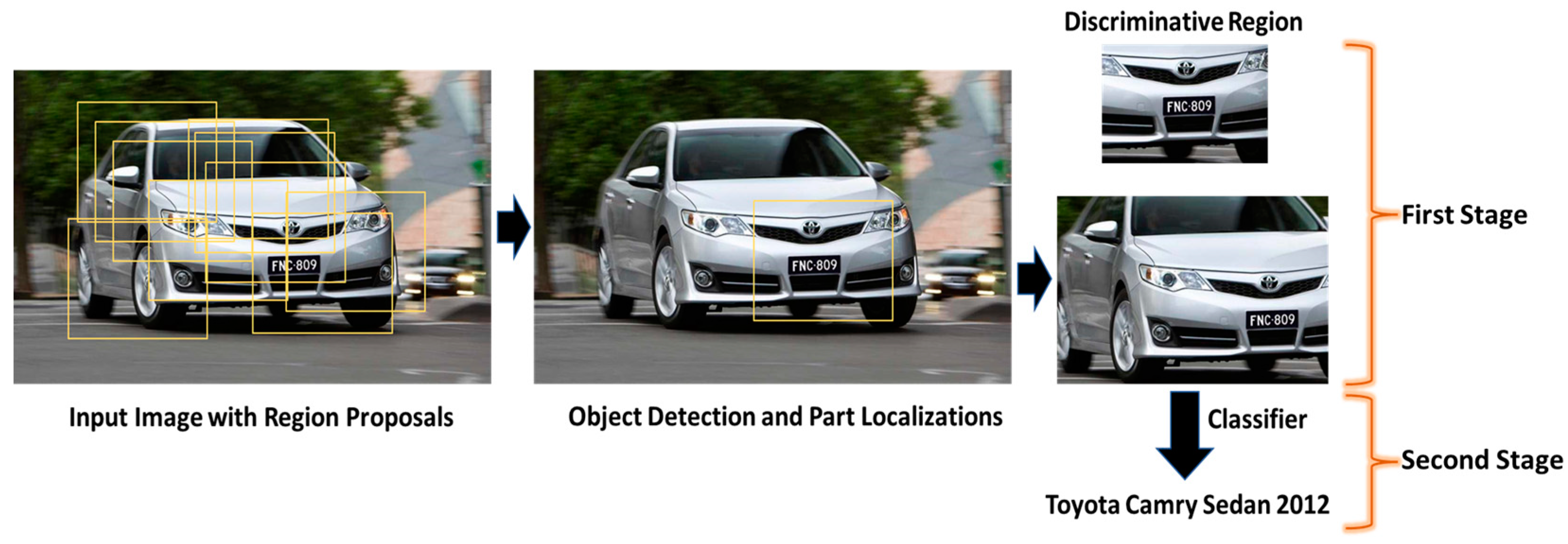
The two-stage method (localization classification subnetworks), in particular, depends on the object and part localization annotations, Region Proposed Networks [
21], or attention mechanisms to acquire discriminatory areas, which are subsequently fed to the classifier. [
22] built object and part detectors using bounding box datasets to find the most effective local semantic parts, and afterward applied a classifier to retrieve final classifications. [
23] generated portions using segmentation and a posture graph, followed by moving them to a classification model. [
24] layered a series of branches comprising a part cascade, an object cascade, and part landmark localization to merge feature maps carrying information from each component along with the bounding box. [
25] combined classification and semantic part recognition. [
26] designed a multi-granularity algorithm for learning with two stages: a targeted search to discover ROI (regions of interest), followed by the classification. [
27] utilized a weakly supervised approach to locate various relevant regions coming from proposals and subsequently apply them to generate a broader representation for classification. The attention mechanism was employed by [
28] to train a coarse-grained model to identify relevant regions, which were then forwarded through a fine-grained network to enhance the categorization. In terms of conclusion, each of those techniques attempts to use object-level or local-level details to eliminate unnecessary information, then feed the relevant information to the classifier for the classification task.
Figure 1 illustrates the basic two-stage method.
Considering the complex two-stage pipeline and the tedious and resource-intensive datasets, the present work emphasizes end-to-end feature encoding through deep learning neural networks to identify the minute differences within subcategories. This strategy relies on maximizing classification outcomes through improved feature representations. A couple of research studies [
29,
30] proposed paired interaction learning approaches to gather semantic differences. [
31] employed the self-attention mechanism, to retrieve discriminative features. [
32] suggested a hierarchical architecture that performs cross-layer bilinear pooling. A small number of studies have focused on fine-grained image recognition task with one-stage object detectors, which similarly adopt the feature encoding approach with the object localization system. Consequently, in this study, we intended to explore the performance and ability of the single-stage detector [
33] on fine-grained image recognition problem to fill the void.
Figure 2 represents the standard layout of end-to-end feature encoding system.
3. Proposed Model
3.1. Yolov5 Backbone
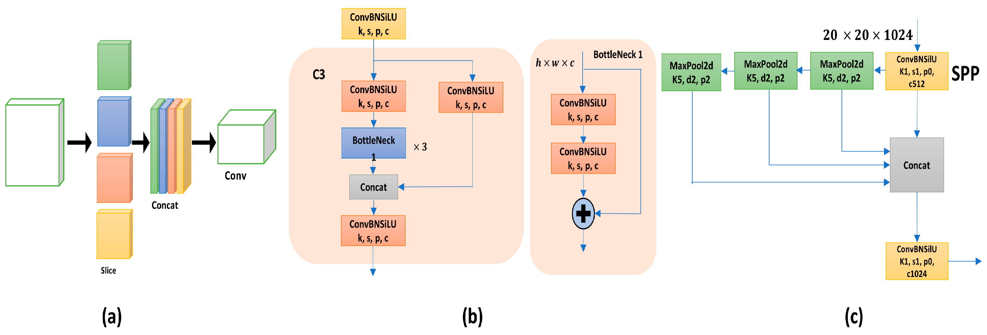
Yolov5 backbone serves the purpose of feature extractor from the given input image. The backbone includes a focused network, spatial pyramid pooling, and a cross-stage partial network, which can be seen in
Figure 3. The Focus structure decreases model parameters and GPU storage space for execution, which results in boosting the model speed. The spatial pyramid pooling unit has the ability to enhance the receptive field. A broad receptive field is capable of spotting the object information and discriminating some of the significant relevant features. Cross-stage partial network has two different kinds of patterns, the difference between them is the reiterated ResUnit, which has more complex layers that are capable of extracting detailed information. Yolov5 backbone, however, struggles with modeling long-range dependencies across the entire input as well as understanding detailed contextual information, which is essential for fine-grained image recognition task. As a result, we proposed an improved backbone by introducing transformer encoder blocks to replace the bottleneck CSP blocks.
3.2. Improved Backbone with Vision Transformer
A traditional vision transformer [
16] is composed of two basic components. a linear projection from an image as well as a transformer encoder block that includes numerous MLP models alongside a self-attention network.
3.2.1. Patch Embedding
The vision transformer method involves splitting the input image into different patches of identical shapes, just like a pattern of embedded words in natural language processing. The image is broken down into image tokens using the vision transformer as
Convolutional neural network employs pixel arrays, however, the patch size
must be specified. This phase involves vectorizing the received visual patches into vectors or flattening them, and then these flattened patches are projected to a lower-dimensional space by using the linear operator on each of the vectors
. Since
and
are two accepted parameters obtained using the training data, these individuals also append a position embedding acquired through patches
to their respective
vectors to ensure that the
vector retains both, the content as well as a position simultaneously. This result is regarded as the patch embeddings and is written as
Through this, nearer patches often have matching position embedding compared to other patches. In recognition tasks, including a second embedded learnable vector into the sequential , that represents the CLS token, enables gathering and keeping data that has been acquired through other tokens and has an identical form like the rest of the vectors.
3.2.2. Transformer Encoder Block
The self-attention mechanism transforms a single feature into another by capturing long-range dependencies across each input by taking
instances with no contextual information and then returns the
entities with the context information. In other terms, it accepts inputs in the manner of
by
, and further employs the learnable weighted matrices that are queries
, keys
, and values
. Evidently, by combining each value with weights after measuring the query across all keys ,the equation below represents the self-attention output.
upon which,
along with SoftMax, to achieve the attention level having
,
, and
using the dot product calculation. Relying on adopting a Self-Attention Layer, the vision transformer applies Multi-Head Self Attention. Where eight headers are often used to streamline various complex connections among different components in a series and handle longer-term dependencies, this corresponds to the aggregated multiple self-attention, that is independent of parameters
,
, and
and possesses similar input, where
and
is the overall length of attention blocks, respectively.
while
=
and
), and outcomes are combined to a single matrix,
.
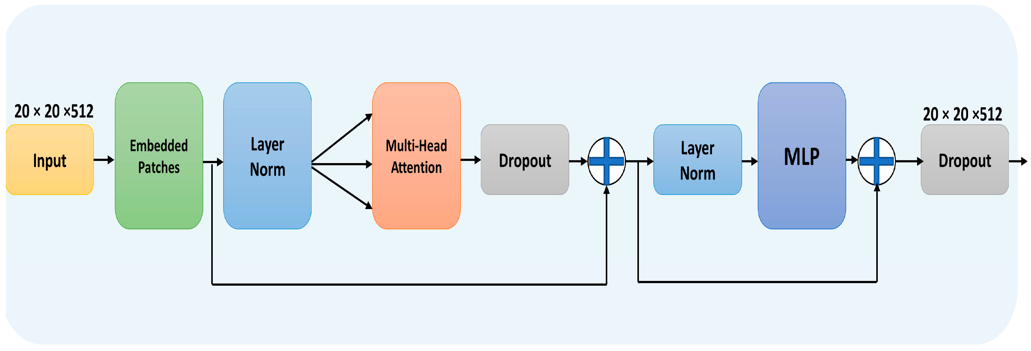
Multilayer Perception (MLP) layers in the transformer encoder block have enabled our model to narrow its attention to the relevant features while minimizing the number of parameters after integrating them into the final layer inside the feature extraction stage. The dimensions of the Input image along with extracted features and the output can be seen in
Figure 4, where
represents the size of the input, and once the input image is converted into a feature map, its dimensions change to
. As a result, the transformer encoder block input size is
. The feature map’s size is
(
) using patch embedding, which applies a simple additive operation through a learnable vector. Therefore, transformer encoder block input vectors and output vectors are of the same size.
3.3. Improved Yolov5
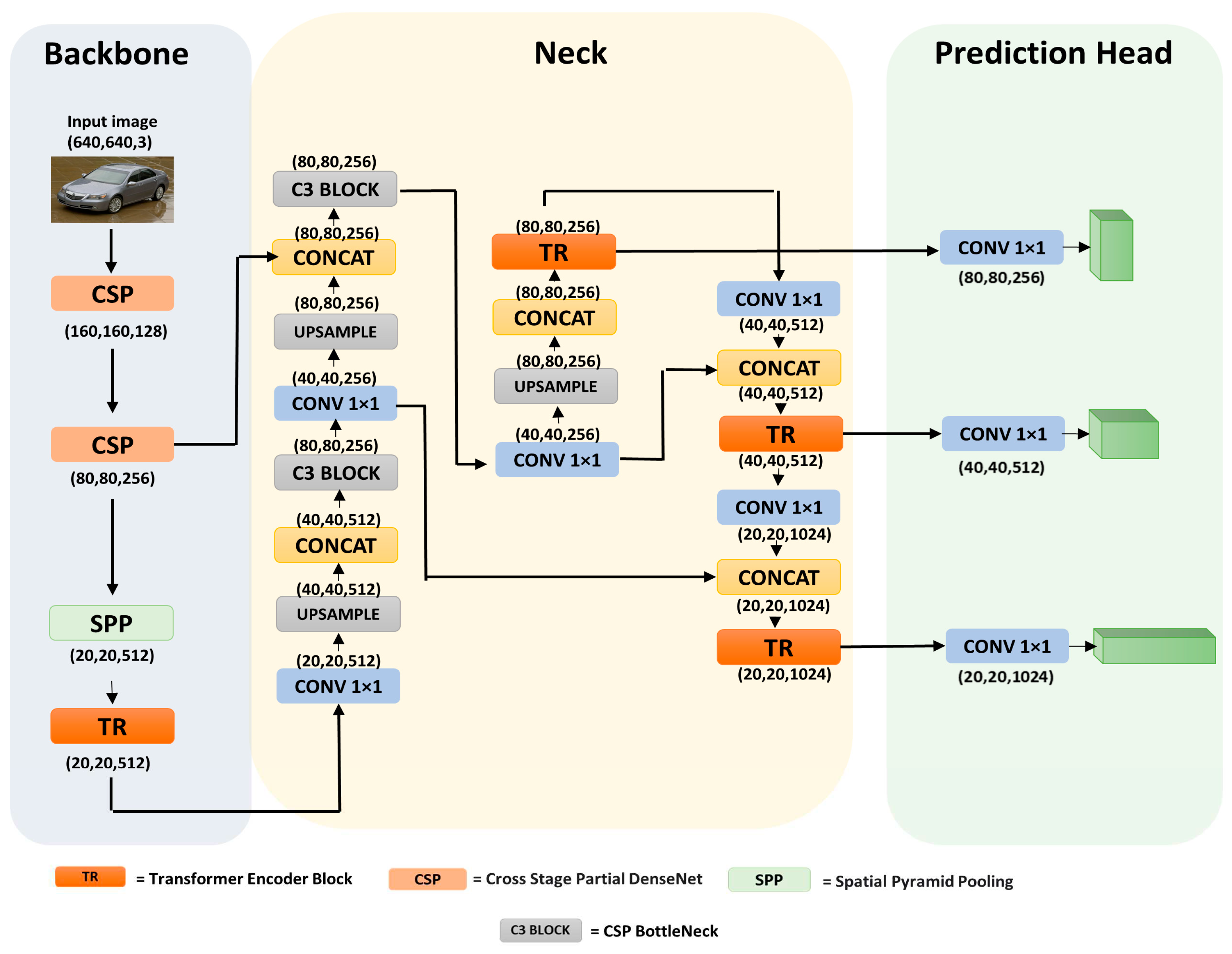
In the Yolov5 model, the learning capability offered by the CSPNet (cross-stage partial network) is used to formulate the CSPDarkNet53 network to boost the network performance. The results greatly minimize the model parameters, simultaneously improve residual feature information, and boost feature learning abilities compared to the ResNet model. While the neck primarily functions to combine information coming from multiple features to form a model with improved representation and richer features. The total number of heads is chosen by the neck, where objects of different sizes are assigned to each head for learning. The neck also maintains a multi-scale feature fusion order that improves the existing range of the features in a more effective manner than utilizing just a single pooling method and notably distinguishes the object context. In our experiment, we also applied the transformer heads at the last stage of the Yolov5 network because the feature maps at that stage have low resolutions, and using transformer heads on low-resolution feature maps reduces high computing costs and memory consumption.
Figure 5 represents the overall proposed architecture for fine-grained image recognition.
4. Model Training and Results
In this section, we will explain the dataset and experiment setup, then exhibit the training outcomes and compare the Yolov5 models. Finally, we will demonstrate the outcomes of the experiment.
4.1. Dataset
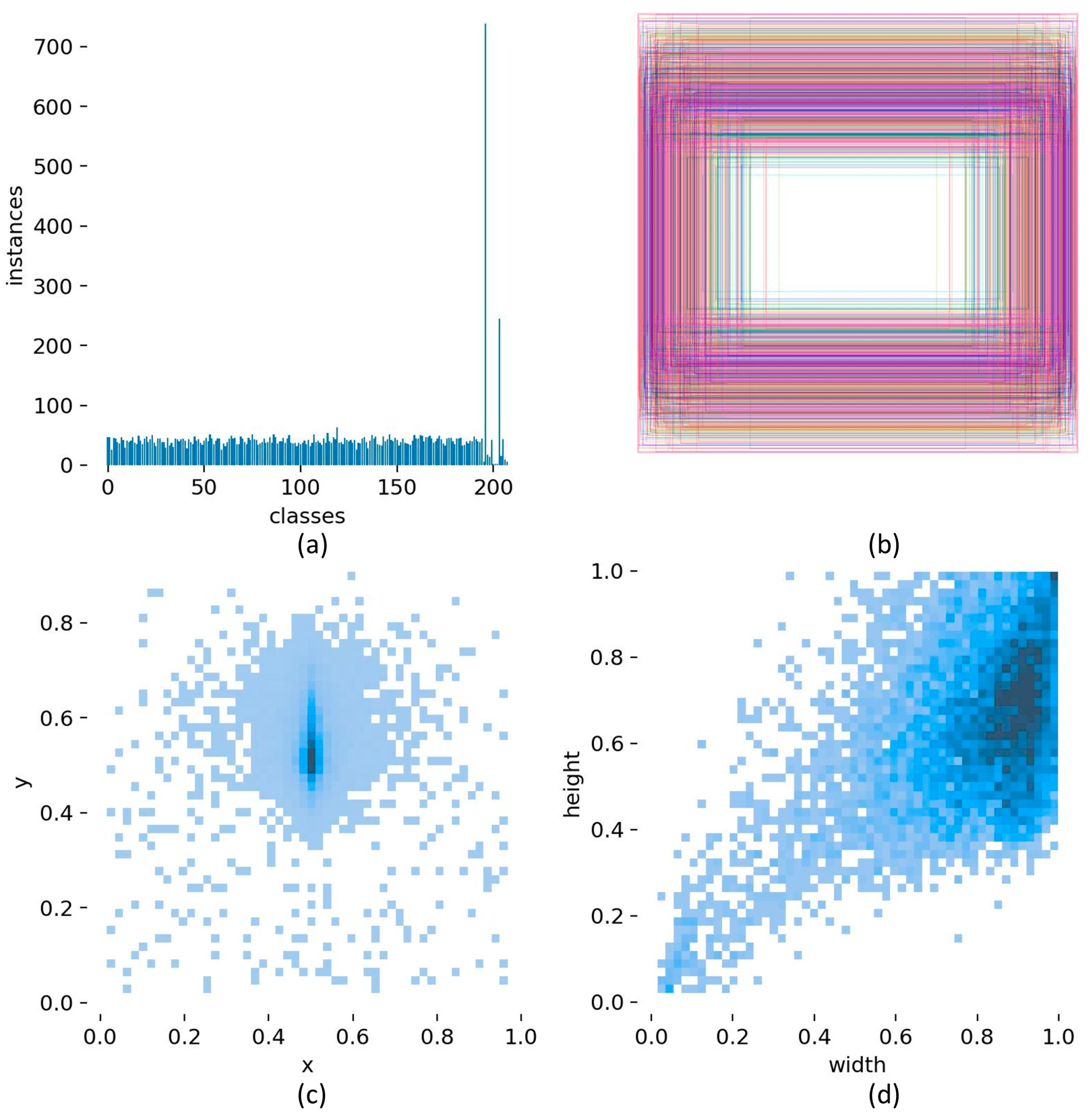
The Stanford car dataset, having 16,185 images of 196 classes and is extended to 208 classes, is used for the experiment. This dataset contains images of vehicle brands with significantly identical visual appearances and is one of the few benchmark datasets that are specifically designed for fine-grained image recognition task. The dataset images, which were in JPEG format and contains different sizes, were first converted into Yolov5 format and then split into train, validation, and test sets.
Figure 6 shows the dataset visualization.
4.2. Experimental Environment
Our training setup involved a window 10 64bit operating system with 13th Gen Intel(R) Core(TM) i5-13400 processor, 32GB of RAM, NVIDIA GeForce RTX 3060 Ti GPU, and Python 3.9 with the Pytorch framework has been utilized. To optimize the performance of our model and to compare and analyze it with Yolov5 existing models, we trained all the models with SGD and ADAM optimizers.
Table 1 displays multiple experimental hyperparameters.
4.3. Evaluation Matrics and Model Training
Precision, Recall, Average Precision, and F1 score are commonly used for statistical analysis to evaluate the effectiveness of the detection model. Below are the equations adopted to evaluate Precision, Recall, and F1 score.
The number of correctly detected objects refers to true positives, false positives are wrongly identified as targets, and false negatives are the number of undetected objects. If the predicted bounding box of an object differs from the ground truth, this is not evidence that the detection is incorrect; therefore, intersection over union (IoU) is a frequent approach, where intersection over union is the ratio of detected bounding box over the ground truth (bounding box). If the value of the IoU is higher than the set threshold, the detection is accurate (true positive); else it is incorrect (false positive).
We derived the F1-Score assuming a harmonic mean of recall and precision upon calculating the precision and recall scores for each class. The F1-Score allows us to understand how the model gets confused while providing predictions. Equation (7) is often used to compute the F1-Score for all classes.
The Precision-Recall Curve represents a curve where the x-coordinate is the recall rate, and the y-coordinate is the accuracy. The total area under Precision-Recall curve is referred to as the average precision (AP), and it can be calculated using Equation (8).
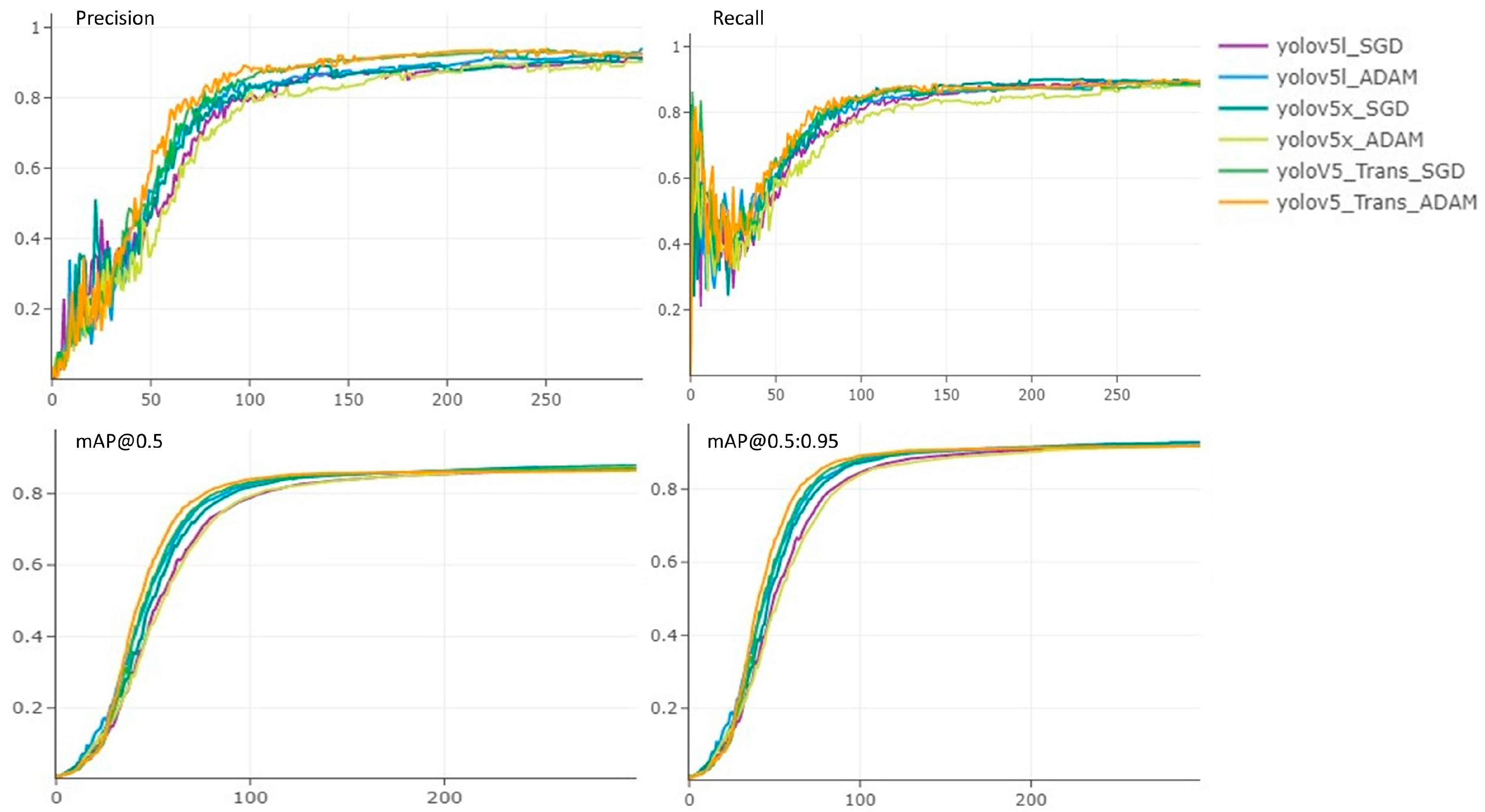
We trained our proposed model using both SGD and ADAM optimizers along with the Yolov5l, and Yolov5x models, which are the existing robust Yolov5 models on the Stanford car training data set. The training results after every epoch are displayed in
Figure 7. It has been observed that during the first training stage, as the training time increased, all six models’ precision increased gradually, while the recall dropped initially, later, the precision of our proposed model increased the fastest, while maintaining the recall high as well.
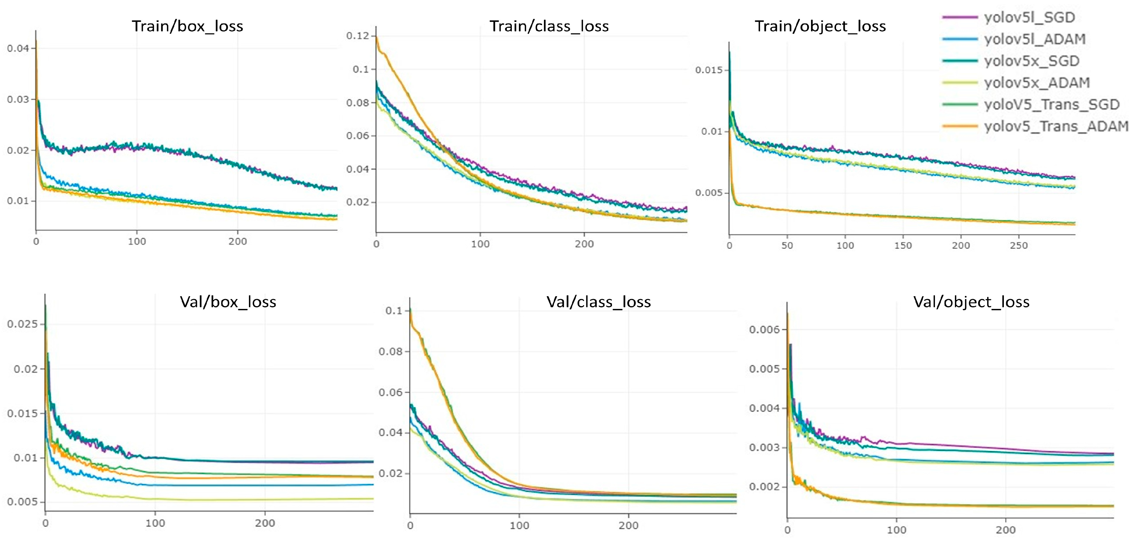
During training and validation, all the losses (object loss, bounding box loss, and class loss) gradually decreased to an acceptable level, as can be seen in
Figure 8 where losses after every epoch are displayed, whereas
Table 2 demonstrates the overall training results of all the six models, which conclude that our model outperforms the other models, among the all trained models, the convergence speed of our proposed Yolov5 with transformer encoder block is more efficient, and the accuracy is higher with minimum losses.
4.4. Model Adaptability over Test Images
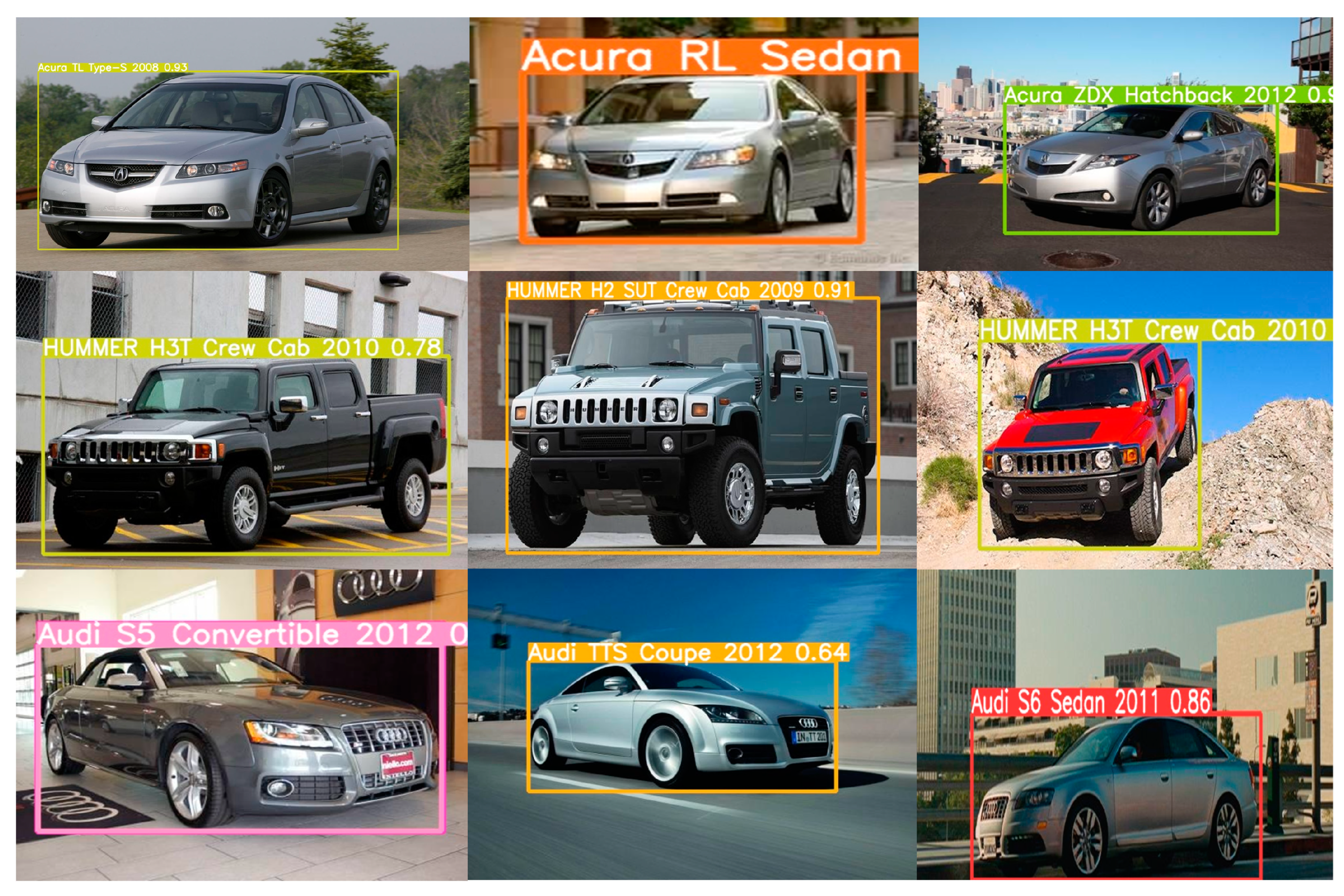
To test our model’s capability for fine-grained image recognition task, we used the Stanford test set, having 1257 challenging identical images. Vehicle recognition results can be seen in
Figure 9.
Table 3 demonstrates our models’ inference speed and compares the result with other trained models. Our model has a slower inference speed as well as preprocessing time compared to Yolov5x, while being slightly higher than the Yolov5l.
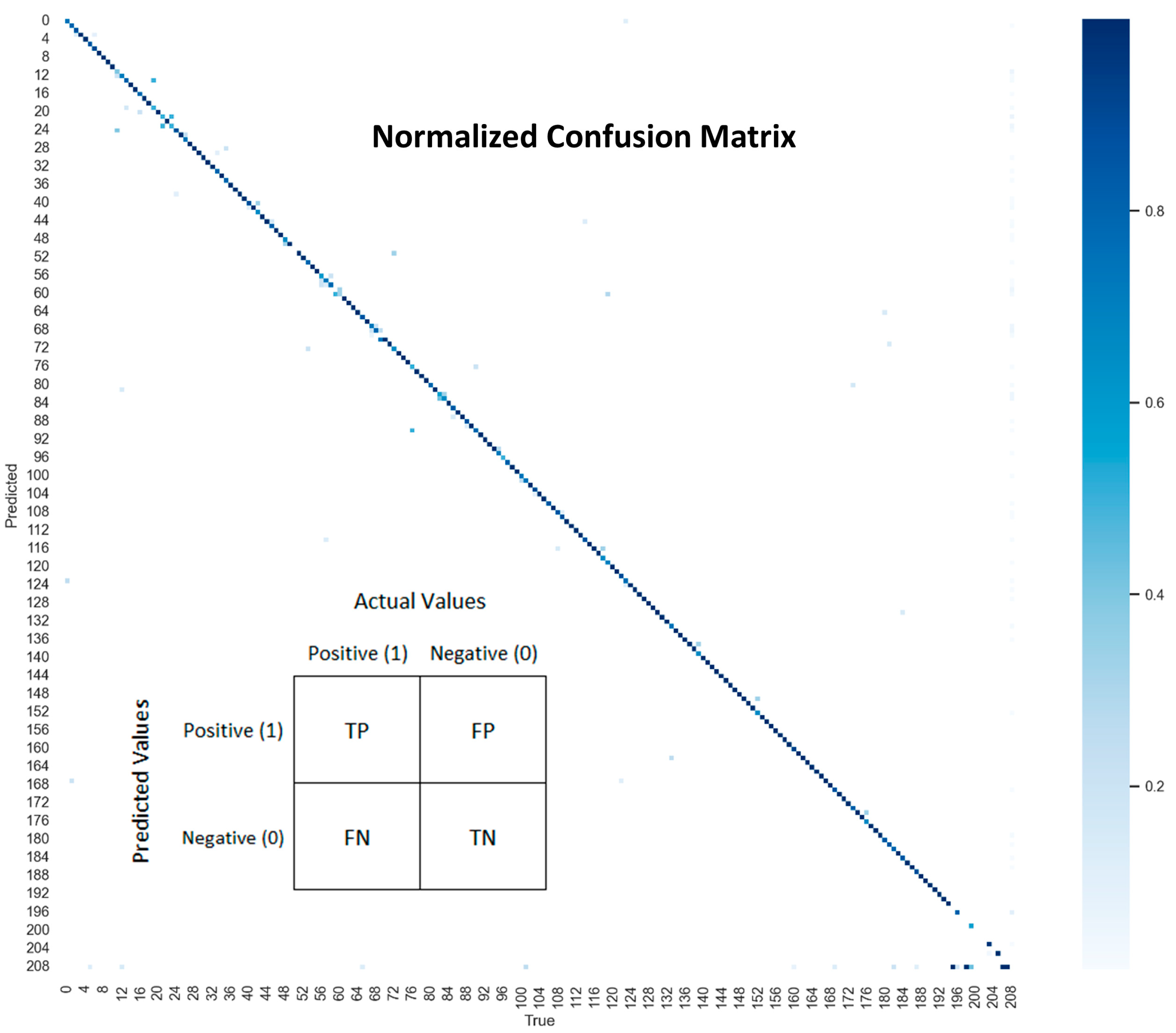
The normalized confusion matrix in
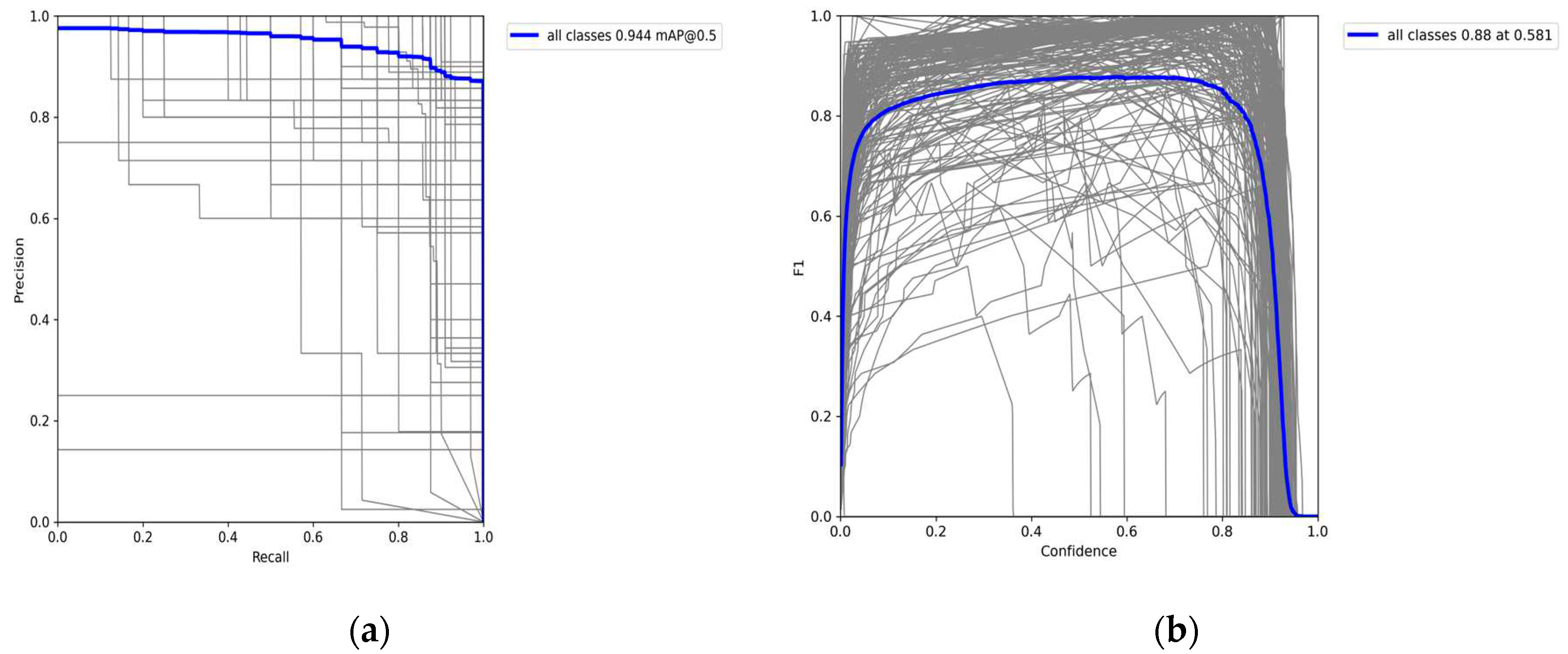
Figure 10 was generated after getting the precision and recall scores for the test images, whereas the precision-recall curve and the F1 confidence score curve for all the classes are produced using Equations (7) and (8) and can be visualized in
Figure 11.
4.5. Compaision with State of the Art
We compared our model with some of the existing state of the art fine-grained image recognition models. Most of the models have utilized the VGG-19 and Resnet-50 backbones and are weakly supervised where no train annotations were employed. The comparison is based on the accuracy achieved using the benchmark Stanford car dataset. Our method achieved 93.4 percent accuracy with an improved CSP-Darknet53 backbone, a comparison can be seen in
Table 4.
5. Limitations
This research focuses on the recognition of fine-grained vehicles, which are almost identical by visualization, although promising results have been achieved using a one- stage object detector, but vision transformers are known for their computational and memory requirements. The self-attention mechanism used in the transformer encoder block computes pairwise interactions between all elements in the input feature map, resulting in quadratic complexity with respect to the input size. During the training stage, our model performed considerably better but still consumed a lot of time because of the more training parameters as compared to the other models, and when we tested the model on the test set, the inference speed was slightly increased as well. The implementation of a visual transformer, which costs speed and additional memory resources, is a drawback of this study. However, as we know, vision transformers divide the input image into fixed-size patches and process them individually. By reducing the patch size, the number of patches and the subsequent memory requirements can be decreased. But taking into consideration that this reduction should be balanced with the model’s ability to capture fine-grained details, as smaller patches might result in a loss of information. Various methods have already been proposed to make transformer attention mechanism more efficient, such as utilizing sparse attention patterns or approximating attention mechanisms with lower complexity operations like kernelized self-attention or linear attention. These approaches can significantly reduce memory requirements and computational overhead and can be considered to align with our future research work.
6. Conclusions
In this paper, we proposed a one-stage fine-grained object recognition model based on Yolov5 object detector. We improved the backbone of the existing Yolov5 model to effectively capture global dependencies and enabled the model to learn relationships between distant regions. This improved the model’s ability to understand the context and captured long-range spatial relationships in the image, which are an important aspect for fine-grained recognition task. We also replaced the Yolov5 detection heads with three transformer heads using the discriminative feature maps from transformer encoder blocks. To evaluate the model improvement after adding the transformer encoder blocks, we used the famous Stanford car dataset, which is a benchmark dataset for fine-grained recognition task consisting of highly similar 16,185 images of 196 different classes of vehicles, which is later updated to 208 classes. We trained the existing Yolov5l and Yolov5x along with our proposed model for 300 iterations using both the stochastic gradient descent (SGD) and adaptive moment estimation (ADAM) optimizers. Evaluation matrices like precision, recall, mAP, and F1 score are used to evaluate the model performance and to get comparisons with the existing Yolov5 and state of the art models. However, further study is required to implement modern vision transformers effectively, particularly to solve the challenges of speed and extreme memory usage.
Author Contributions
Conceptualization, U.A. and S.O.; methodology, U.A.; software, U.A.; validation, J.K., T.W. and M.H.; formal analysis, J.K.; investigation, U.A.; resources, S.O.; data curation, U.A.; writing—original draft preparation, U.A.; writing—review and editing, J.K.; visualization, T.W.; supervision, J.K.; project administration, S.O.; funding acquisition, J.K. All authors have read and agreed to the published version of the manuscript.
Funding
This work was funded by the Korea government(MSIT) (2022-0-00215). This work was supported by the Institute of Information & communications Technology Planning & Evaluation (IITP) grant funded by the Korea government(MSIT) (2021-0-02068, Artificial Intelligence Innovation Hub).
Institutional Review Board Statement
Not applicable.
Informed Consent Statement
Not applicable.
Data Availability Statement
Not applicable.
Conflicts of Interest
The authors declare no conflict of interest.
References
- K. Pang, Y. Yang, T. M. Hospedales, T. Xiang, and Y. Z. Song, “Solving Mixed-Modal Jigsaw Puzzle for Fine-Grained Sketch-Based Image Retrieval,” Proceedings of the IEEE Computer Society Conference on Computer Vision and Pattern Recognition, pp. 10344–10352, 2020. [CrossRef]
- W. Zhou et al., “Fashion recommendations through cross-media information retrieval,” J Vis Commun Image Represent, vol. 61, pp. 112–120, May 2019. [CrossRef]
- W. Min, S. Jiang, and R. Jain, “Food Recommendation: Framework, Existing Solutions, and Challenges,” IEEE Trans Multimedia, vol. 22, no. 10, pp. 2659–2671, Oct. 2020. [CrossRef]
- J. Bao, D. Chen, F. Wen, H. Li, and G. Hua, “CVAE-GAN: Fine-Grained Image Generation through Asymmetric Training,” Proceedings of the IEEE International Conference on Computer Vision, vol. 2017-October, pp. 2764–2773, Dec. 2017. [CrossRef]
- L. Jing, X. Yang, and Y. Tian, “Video you only look once: Overall temporal convolutions for action recognition,” J Vis Commun Image Represent, vol. 52, pp. 58–65, Apr. 2018. [CrossRef]
- N. Xu, A. A. Liu, J. Liu, W. Nie, and Y. Su, “Scene graph captioner: Image captioning based on structural visual representation,” J Vis Commun Image Represent, vol. 58, pp. 477–485, Jan. 2019. [CrossRef]
- Z. Qin, Y. Zhang, S. Meng, Z. Qin, and K. K. R. Choo, “Imaging and fusing time series for wearable sensor-based human activity recognition,” Information Fusion, vol. 53, pp. 80–87, Jan. 2020. [CrossRef]
- K. Simonyan and A. Zisserman, “Very Deep Convolutional Networks for Large-Scale Image Recognition,” 3rd International Conference on Learning Representations, ICLR 2015 - Conference Track Proceedings, Sep. 2014, Accessed: May 22, 2023. [Online]. Available: https://arxiv.org/abs/1409.1556v6.
- B. Zhao, X. Wu, J. Feng, Q. Peng, and S. Yan, “Diversified Visual Attention Networks for Fine-Grained Object Classification,” IEEE Trans Multimedia, vol. 19, no. 6, pp. 1245–1256, Jun. 2017. [CrossRef]
- Dubey, O. Gupta, P. Guo, R. Raskar, R. Farrell, and N. Naik, “Pairwise Confusion for Fine-Grained Visual Classification,” Lecture Notes in Computer Science (including subseries Lecture Notes in Artificial Intelligence and Lecture Notes in Bioinformatics), vol. 11216 LNCS, pp. 71–88, May 2017. [CrossRef]
- Yu, X. Zhao, Q. Zheng, P. Zhang, and X. You, “Hierarchical Bilinear Pooling for Fine-Grained Visual Recognition,” Lecture Notes in Computer Science (including subseries Lecture Notes in Artificial Intelligence and Lecture Notes in Bioinformatics), vol. 11220 LNCS, pp. 595–610, Jul. 2018. [CrossRef]
- R. Ji et al., “Attention Convolutional Binary Neural Tree for Fine-Grained Visual Categorization,” Proceedings of the IEEE Computer Society Conference on Computer Vision and Pattern Recognition, pp. 10465–10474, Sep. 2019. [CrossRef]
- J. Fu, H. Zheng, and T. Mei, “Look closer to see better: Recurrent attention convolutional neural network for fine-grained image recognition,” Proceedings - 30th IEEE Conference on Computer Vision and Pattern Recognition, CVPR 2017, vol. 2017-January, pp. 4476–4484, Nov. 2017. [CrossRef]
- X. Zhang, H. Xiong, W. Zhou, W. Lin, and Q. Tian, “Picking deep filter responses for fine-grained image recognition,” Proceedings of the IEEE Computer Society Conference on Computer Vision and Pattern Recognition, vol. 2016-December, pp. 1134–1142, Dec. 2016. [CrossRef]
- Q. Jiao, Z. Liu, L. Ye, and Y. Wang, “Weakly labeled fine-grained classification with hierarchy relationship of fine and coarse labels,” J Vis Commun Image Represent, vol. 63, Aug. 2019. [CrossRef]
- Dosovitskiy et al., “An Image is Worth 16x16 Words: Transformers for Image Recognition at Scale,” Oct. 2020, Accessed: May 23, 2023. [Online]. Available: https://arxiv.org/abs/2010.11929v2.
- S. Zheng et al., “Rethinking Semantic Segmentation from a Sequence-to-Sequence Perspective with Transformers,” Proceedings of the IEEE Computer Society Conference on Computer Vision and Pattern Recognition, pp. 6877–6886, Dec. 2020. [CrossRef]
- J. Chen et al., “TransUNet: Transformers Make Strong Encoders for Medical Image Segmentation,” Feb. 2021, Accessed: May 23, 2023. [Online]. Available: https://arxiv.org/abs/2102.04306v1.
- N. Carion, F. Massa, G. Synnaeve, N. Usunier, A. Kirillov, and S. Zagoruyko, “End-to-End Object Detection with Transformers,” Lecture Notes in Computer Science (including subseries Lecture Notes in Artificial Intelligence and Lecture Notes in Bioinformatics), vol. 12346 LNCS, pp. 213–229, May 2020. [CrossRef]
- Bochkovskiy, C.-Y. Wang, and H.-Y. M. Liao, “YOLOv4: Optimal Speed and Accuracy of Object Detection,” Apr. 2020, Accessed: May 24, 2023. [Online]. Available: https://arxiv.org/abs/2004.10934v1.
- S. Ren, K. He, R. Girshick, and J. Sun, “Faster R-CNN: Towards Real-Time Object Detection with Region Proposal Networks,” IEEE Trans Pattern Anal Mach Intell, vol. 39, no. 6, pp. 1137–1149, Jun. 2015. [CrossRef]
- N. Zhang, J. Donahue, R. Girshick, and T. Darrell, “Part-based R-CNNs for Fine-grained Category Detection,” Lecture Notes in Computer Science (including subseries Lecture Notes in Artificial Intelligence and Lecture Notes in Bioinformatics), vol. 8689 LNCS, no. PART 1, pp. 834–849, Jul. 2014. [CrossRef]
- J. Krause, H. Jin, J. Yang, and F. F. Li, “Fine-grained recognition without part annotations,” Proceedings of the IEEE Computer Society Conference on Computer Vision and Pattern Recognition, vol. 07-12-June-2015, pp. 5546–5555, Oct. 2015. [CrossRef]
- S. Huang, Z. Xu, D. Tao, and Y. Zhang, “Part-Stacked CNN for Fine-Grained Visual Categorization,” Proceedings of the IEEE Computer Society Conference on Computer Vision and Pattern Recognition, vol. 2016-December, pp. 1173–1182, Dec. 2015. [CrossRef]
- H. Zhang et al., “SPDA-CNN: Unifying semantic part detection and abstraction for fine-grained recognition,” Proceedings of the IEEE Computer Society Conference on Computer Vision and Pattern Recognition, vol. 2016-December, pp. 1143–1152, Dec. 2016. [CrossRef]
- D. Wang, Z. Shen, J. Shao, W. Zhang, X. Xue, and Z. Zhang, “Multiple Granularity Descriptors for Fine-Grained Categorization,” in 2015 IEEE International Conference on Computer Vision (ICCV), IEEE, Dec. 2015, pp. 2399–2406. [CrossRef]
- Y. Zhang et al., “Weakly supervised fine-grained categorization with part-based image representation,” IEEE Transactions on Image Processing, vol. 25, no. 4, pp. 1713–1725, Apr. 2016. [CrossRef]
- E. Eshratifar, D. Eigen, M. Gormish, and M. Pedram, “Coarse2Fine: A Two-stage Training Method for Fine-grained Visual Classification,” Mach Vis Appl, vol. 32, no. 2, Sep. 2019. [CrossRef]
- P. Zhuang, Y. Wang, and Y. Qiao, “Learning Attentive Pairwise Interaction for Fine-Grained Classification,” AAAI 2020 - 34th AAAI Conference on Artificial Intelligence, pp. 13130–13137, Feb. 2020. [CrossRef]
- H. Zheng, J. Fu, Z. J. Zha, and J. Luo, “Learning Deep Bilinear Transformation for Fine-grained Image Representation,” Adv Neural Inf Process Syst, vol. 32, Nov. 2019, Accessed: May 25, 2023. [Online]. Available: https://arxiv.org/abs/1911.03621v1.
- J. He et al., “TransFG: A Transformer Architecture for Fine-grained Recognition,” Proceedings of the 36th AAAI Conference on Artificial Intelligence, AAAI 2022, vol. 36, pp. 1174–1182, Mar. 2021. [CrossRef]
- C. Yu, X. Zhao, Q. Zheng, P. Zhang, and X. You, “Hierarchical Bilinear Pooling for Fine-Grained Visual Recognition,” Lecture Notes in Computer Science (including subseries Lecture Notes in Artificial Intelligence and Lecture Notes in Bioinformatics), vol. 11220 LNCS, pp. 595–610, Jul. 2018. [CrossRef]
- G. Jocher et al., “ultralytics/yolov5: v7.0 - YOLOv5 SOTA Realtime Instance Segmentation,” Nov. 2022. [CrossRef]
Figure 1.
Localization classification method based on two stages.
Figure 1.
Localization classification method based on two stages.
Figure 2.
Simple End-to-End Feature Encoding method.
Figure 2.
Simple End-to-End Feature Encoding method.
Figure 3.
(a) Focus network, (b) BottleNeckCSP module, (c) Spatial Pyramid Pooling.
Figure 3.
(a) Focus network, (b) BottleNeckCSP module, (c) Spatial Pyramid Pooling.
Figure 4.
Transformer Encoder Block performs the additive operation through a learnable vector and has the same input and output size.
Figure 4.
Transformer Encoder Block performs the additive operation through a learnable vector and has the same input and output size.
Figure 5.
Proposed model based on Yolov5 for fine-grained image recognition task. Three transformer encoder blocks have been added at the end of the backbone, where input features are fed through a spatial pyramid pooling layer. Replaced Transformer Predictions heads take the feature maps from the neck part.
Figure 6.
Visualization of the dataset. (a) the number of annotations for each class; (b) a visual representation of the location as well as the dimensions associated with each bounding box (c) The Statistical distribution of bounding box location. (d) Statistical distribution of bounding box dimensions.
Figure 7.
All models’ training results after every epoch. Proposed model Precision during training peaked at 0.934 along with the recall of 0.895 where average precision at 0.5 and 0.5:0.95 threshold peaked at 0.927 and 0.878 respectively.
Figure 7.
All models’ training results after every epoch. Proposed model Precision during training peaked at 0.934 along with the recall of 0.895 where average precision at 0.5 and 0.5:0.95 threshold peaked at 0.927 and 0.878 respectively.
Figure 8.
Representation of all models’ training losses after every epoch. Our proposed model along with the Yolov5x model with the Adam optimizer had minimum losses (box, class, object) during training and validation.
Figure 8.
Representation of all models’ training losses after every epoch. Our proposed model along with the Yolov5x model with the Adam optimizer had minimum losses (box, class, object) during training and validation.
Figure 9.
Proposed models’ recognition results with similar shapes vehicles but different brand models and make year. The model performed better when provided with similar vehicle shapes and colors at different viewing angles.
Figure 9.
Proposed models’ recognition results with similar shapes vehicles but different brand models and make year. The model performed better when provided with similar vehicle shapes and colors at different viewing angles.
Figure 10.
Proposed model confusion matrix based on the test set predictions. As can be seen in the Figure, the diagonal values are the correctly predicted samples.
Figure 10.
Proposed model confusion matrix based on the test set predictions. As can be seen in the Figure, the diagonal values are the correctly predicted samples.
Figure 11.
PR curve and F1 confidence score curve from the proposed model’s test set recognition results. (a) represents the mAP@0.5 threshold for all classes where the average precision is 0.944. (b) represents the proposed model confidence score of 0.88 at the 0.581 threshold value.
Figure 11.
PR curve and F1 confidence score curve from the proposed model’s test set recognition results. (a) represents the mAP@0.5 threshold for all classes where the average precision is 0.944. (b) represents the proposed model confidence score of 0.88 at the 0.581 threshold value.
Table 1.
Experiment Hyperparameters details, most of the parameters were set to the same as the default Yolov5 model, only data loaders and optimizers were tested at different stages.
Table 1.
Experiment Hyperparameters details, most of the parameters were set to the same as the default Yolov5 model, only data loaders and optimizers were tested at different stages.
| Parameter |
Values |
| Batch Size |
16 |
| Learning Rate |
0.01 |
| Learning Rate Decay |
0.999 |
| Momentum |
0.937 |
| Learning Rate Decay Step |
5.e-4 |
| Epoch |
300 |
| Workers |
8 |
Table 2.
Overall training results for all the models. Our proposed model improved in every aspect during the training process, whereas Yolov5x has slightly improved with the ADAM optimizer.
Table 2.
Overall training results for all the models. Our proposed model improved in every aspect during the training process, whereas Yolov5x has slightly improved with the ADAM optimizer.
| Model |
Precision |
Recall |
mAP
@0.5 |
mAP
0.5:0.95 |
| Yolov5l_SGD |
0.890 |
0.885 |
0.912 |
0.863 |
| Yolov5l_ADAM |
0.911 |
0.880 |
0.912 |
0.864 |
| Yolov5x_SGD |
0.896 |
0.889 |
0.917 |
0.874 |
| Yolov5x_ADAM |
0.901 |
0.891 |
0.919 |
0.868 |
| Yolov5_tr_SGD |
0.931 |
0.892 |
0.921 |
0.873 |
| Yolov5l_tr_ADAM |
0.934 |
0.895 |
0.927 |
0.878 |
Table 3.
All models’ inference speed comparison on the Stanford car test set. Yolov5l, with fewer training parameters, has the edge of being a lighter model that can detect at a minimum inference speed of 15.5 ms, but recognition accuracy is lower than that of our proposed model, which is slightly behind by 39.2 ms.
| Model |
Pre-process(ms) |
Inference Speed(ms) |
NMS/
Image(ms) |
Image Size |
| Yolov5l_SGD |
0.3 |
15.5 |
0.6 |
640 × 640 |
| Yolov5l_ADAM |
0.3 |
15.5 |
0.6 |
640 × 640 |
| Yolov5x_SGD |
0.3 |
28.7 |
0.7 |
640 × 640 |
| Yolov5x_ADAM |
0.4 |
28.4 |
0.7 |
640 × 640 |
| Yolov5_tr_SGD |
0.8 |
39.2 |
0.9 |
640 × 640 |
| Yolov5l_tr_ADAM |
0.8 |
39.2 |
0.9 |
640 × 640 |
Table 4.
Accuracy comparison of our model with the state of the art on Stanford car dataset.
Table 4.
Accuracy comparison of our model with the state of the art on Stanford car dataset.
| Methods |
Train Anno |
Backbone |
Image
Resolution |
Accuracy
|
| RA-CNN |
|
VGG-19 |
448 × 448 |
92.5% |
| BoT |
|
Alex-Net |
Not given |
92.5% |
| WPA |
BBox |
CaffeNet |
224×224 |
92.6% |
| MA-CNN |
|
VGG-19 |
448 × 448 |
92.8% |
| PA-CNN |
|
VGG-19 |
448 × 448 |
93.3% |
| M2DRL |
|
VGG-16 |
448 × 448 |
93.3% |
| Yolov5-Trans |
BBox |
CSP-Darknet53 |
640×640
|
93.4% |
| DFL-CNN |
|
VGG-16 |
448 × 448 |
93.8% |
| TASN |
|
ResNet-50 |
224 × 224 |
93.8% |
| Hsnet |
Parts |
GoogleNet |
224 × 224 |
93.9% |
| MGE-CNN |
|
ResNet-50 |
448 × 448 |
93.9% |
| NTS-Net |
|
ResNet-50 |
448 × 448 |
93.9% |
| GCL |
|
ResNet-50+BN |
448 × 448 |
94.0% |
| FDL |
|
ResNet-50 |
448 × 448 |
94.3% |
| S3N |
|
ResNet-50 |
448 × 448 |
94.7% |
| DF-GMM |
|
ResNet-50 |
448 × 448 |
94.8% |
|
Disclaimer/Publisher’s Note: The statements, opinions and data contained in all publications are solely those of the individual author(s) and contributor(s) and not of MDPI and/or the editor(s). MDPI and/or the editor(s) disclaim responsibility for any injury to people or property resulting from any ideas, methods, instructions or products referred to in the content. |
© 2023 by the authors. Licensee MDPI, Basel, Switzerland. This article is an open access article distributed under the terms and conditions of the Creative Commons Attribution (CC BY) license (http://creativecommons.org/licenses/by/4.0/).
