1. Introduction
MPC is an effective control method developed in industrial practice. It can well deal with the problems of multivariable, multi-constraint, strong coupling, and strong nonlinearity existing in actual industrial process objects, it has been widely concerned by academia and industry and resulted in numerous theoretical research and application results [
1,
2]. The MPC method predicts the system’s future behavior based on the controlled object’s dynamic model to achieve the goal of optimal control. Therefore, the predictive model's capacity to describe the system has a substantial effect on the MPC controller's control performance. Due to the fact that some key parameters of complex nonlinear systems cannot be determined or obtained, it’s difficult to obtain the physical model that accurately represents the system’s nonlinear dynamic characteristics by establishing differential or difference equations through Newtonian mechanics analysis or Lagrange energy method [
3]. Therefore, data-driven identification is a highly effective modeling approach to realize the MPC of nonlinear systems. This method uses input and output data to construct the system model and does not need to analyze the complex interrelationship between the various physical variables of the system [
4,
5].
When designing predictive control algorithms based on the identified nonlinear system models, using the segmented linearization [
6] or local linearization [
7] models can simplify the controller's design, but can not well represent the complex system’s nonlinear dynamic characteristics, which will affect the control performance of the controller. To address the accuracy loss issue caused by linearization models, direct use of nonlinear models such as bilinear models [
8,
9], Volterra series models [
10,
11], and neural network models [
12,
13] can provide a better description of the system's nonlinear dynamic characteristics. However, predictive control algorithms based on these nonlinear models online solving of non-convex nonlinear optimization problems, which may increase the computational burden and may not guarantee feasible solutions. To address these issues, in recent years, many scholars have started studying combined models, including the Hammerstein model [
14], Wiener model [
15], Hammerstein-Wiener model [
16,
17], and SD-ARX model [18–25]. Among them, the SD-ARX model outperforms the Hammerstein and Wiener models in capturing the nonlinear system's dynamic properties. The SD-ARX model uses state-dependent coefficients to represent the system’s nonlinear dynamic properties, and its local linear and global nonlinear structural characteristics make it easy to design MPC controllers. In recent years, SD-ARX models obtained by fitting model coefficients using RBF neural networks [18–23], deep belief networks [
24], and wavelet neural networks [
25] have been widely employed for complex industrial system modeling and control. However, these neural networks belong to feedforward neural networks, and their data information can only be transmitted forward, and the connection between network nodes at each layer does not form a cycle, so their ability to describe nonlinear systems is limited.
With the fast advancement of AI technology, deep learning has attained success in numerous fields [
26]. Its core idea is to learn the high-dimensional features of data through multi-level nonlinear transformation and a back-propagation algorithm. LSTM and CNN are popular deep learning neural networks, but their design objectives and application scenarios are different. LSTM is primarily employed for time series modeling and has strong memory ability and long-term dependence, and has achieved great success in natural language processing [27–29], speech recognition [30–32], time series prediction [
33,
34,
35,
36], etc. Because LSTM neural network introduces a gating mechanism, it successfully solves the issue of gradient vanishing and exploding in standard recurrent neural network (RNN), allowing it to process long sequence data more efficiently, which is conducive to nonlinear systems modeling. For example, Wu et al. [
37] developed a dropout LSTM and co-teaching LSTM strategy for nonlinear systems. Terzi et al. [
38] developed an MPC method based on the LSTM network and carried out numerical tests on the pH reactor simulator. Zarzycki et al. [
39] developed a model prediction algorithm based on the LSTM network, which achieved good modeling accuracy and control effect by using online advanced tracking linearization. Although these modeling methods based on LSTM neural network can well learn the time dimension features in nonlinear system data, the ability to learn the spatial dimension features is limited, which affects the accuracy of system modeling. In addition, the validation of these methods has been proved by numerical simulation only, but not yet applied to real objects.
The CNN can autonomously learn the spatial features of input data through convolution and pooling operations and is mainly used in computer vision [
40,
41,
42,
43]. Therefore, the composite neural network consisting of LSTM and CNN can effectively learn the spatiotemporal features of data and improve the accuracy of complex nonlinear modeling. Its research mainly focuses on emotion analysis [
44,
45,
46] and text classification [
47,
48,
49] and has not been found to be used for modeling and MPC of real industrial objects.
This article established the LSTM-ARX and LSTM-CNN-ARX models to represent a category of smooth nonlinear systems whose operating point may change over time, and its nonlinear characteristics can be locally linearized by using LSTM or/and CNN to fit the SD-ARX model's coefficients. Furthermore, according to the pseudo-linear structure of the SD-ARX model that exhibits both local linearization and global nonlinearity, two model predictive controllers have been designed, namely LSTM-ARX-MPC and LSTM-CNN-ARX-MPC. To evaluate the performance of these models and control algorithms, a real-time control comparative study was conducted on the commonly used water tank system (WTS) in industrial process control. The outcomes showed that the developed models and MPC algorithms are effective and feasible. Particularly, the LSTM-CNN-ARX-MPC demonstrates excellent comprehensive control performance by leveraging the strengths of LSTM for learning temporal dimension characteristics and CNN for learning spatial dimension characteristics, enabling it to efficiently and accurately learn the nonlinear system’s spatiotemporal characteristics from large volumes of data. This article's major contributions are summarized below.
1) The LSTM-ARX and LSTM-CNN-ARX models are proposed to describe the system's nonlinear features.
2) The predictive controller was developed using the model's pseudo-linear structure features.
3) Control comparison experiments were conducted on the WTS, which is a commonly used industrial process control device, to validate the efficiency of the developed models and control algorithms. To our knowledge, there are currently no reports on using deep learning algorithms for nonlinear systems modeling and real-time control of actual industrial equipment. This study demonstrates how to establish deep learning-related models for nonlinear systems, design the MPC algorithms, and achieve real-time control rather than only doing a numerical simulation as in relevant literature.
The article's structure is as below. Sect. 2 describes the related work. Sect. 3 studies three combination models. Sect. 4 designs the model-based predictive controllers. Sect. 5 presents the results of real-time control comparative experiments on WTS. Sect. 6 summarizes the research content.
2. Related Work
The SD-ARX, LSTM, and CNN models are summarized in this part.
2.1. SD-ARX model
The nonlinear ARX model is used to represent a category of smooth nonlinear systems as below: [
23]:
where
represents output,
represents input,
represents white noise,
and
represent model orders. At an operating point
,
is expanded into the following Taylor polynomial
Then, substituting equation (2) into equation (1) yields the SD-ARX model as follows.
where
,
and
represent the regression coefficients that can be obtained by fitting using neural networks, including BRF neural networks [
18,
19,
20,
21,
22,
23] and wavelet neural networks [
24].
represents the operating state at time
, which may correspond to the system's input or/and output. When fixing
, equation (3) is considered a locally linearized model, and when
varies with the system's operating point, equation (3) represents a model capable of globally describing the system's nonlinear properties. This model has local linear and global nonlinear features, making it advantageous for MPC design. In this article, we use LSTM or/and CNN to approximate the model’s regression coefficients and obtain a category of SD-ARX models that can effectively represent the system's nonlinear properties.
2.2. LSTM
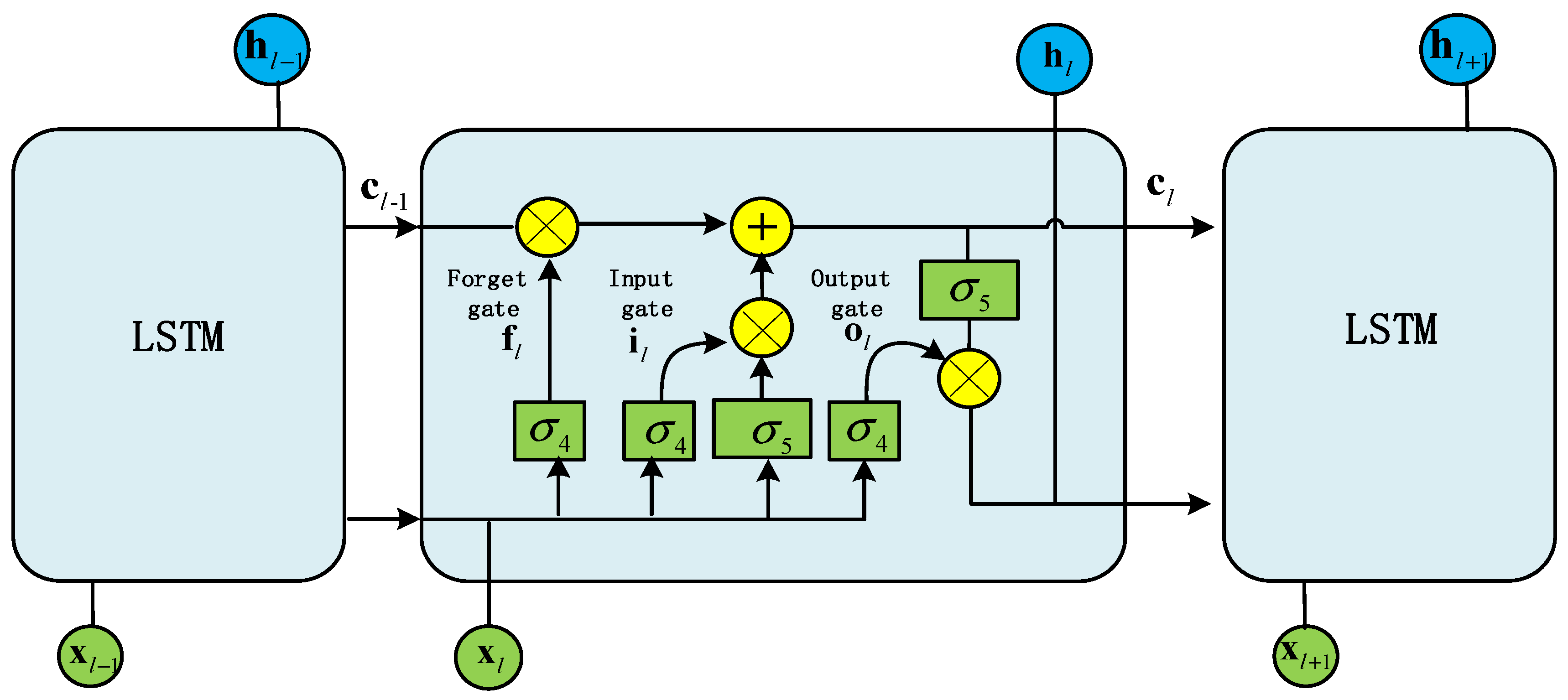
LSTM network serves as an upgraded variant of RNN, which can not only solve the problem that traditional RNN cannot handle the dependence of long sequence data, but also solve the issue that gradient exploding or vanishing is easy to occur with increasing training time and network layers of the neural networks. The LSTM network consists of multiple LSTM units, and its internal structure and chain structure are shown in
Figure 1, with its core being the cell state
, represented by a horizontal line running through the entire cell at the top layer. It controls the addition or removal of information through gates. LSTM mainly consists of an input gate, a forget gate, and an output gate. The input gate controls which input information needs to be added to the current time step's storage unit, the forget gate controls which information needs to be forgotten in the storage unit of the previous time step, and the output gate controls which information in the current time step's storage unit needs to be output to the next time step. LSTM introduces a gate mechanism to control information transmission, remember content that needs to be memorized for a long time, and forget unimportant information, making it particularly effective in handling and forecasting critical events with long intervals and temporal delays in sequential data. The formula for an LSTM unit is as follows.
where
represents the time step of the input sequence, referred to as the number of rounds;
represents matrix dot multiplication;
and
denotes cell state vector and hidden state vector, respectively;
and
denotes the nonlinear activation functions;
represents input information;
represents the forget gate’s output, which decides the amount of information from the preceding state
needs to be forgotten. The value of the output ranges from 0 to 1, with a smaller value indicating more information to be forgotten, 0 means total forgetting, and 1 means total retention;
indicates the input gate's output, which controls the current output state. Its output value is usually mapped to a range of 0 to 1 using the
function, indicating the degree of activation of the output state, with 1 indicating full activation and 0 indicating no activation;
represents the output gate's output, which decides the information to be output in this round;
,
,
,
,
,
,
and
denote weight coefficients,
,
,
and
denote offsets.
2.3. CNN
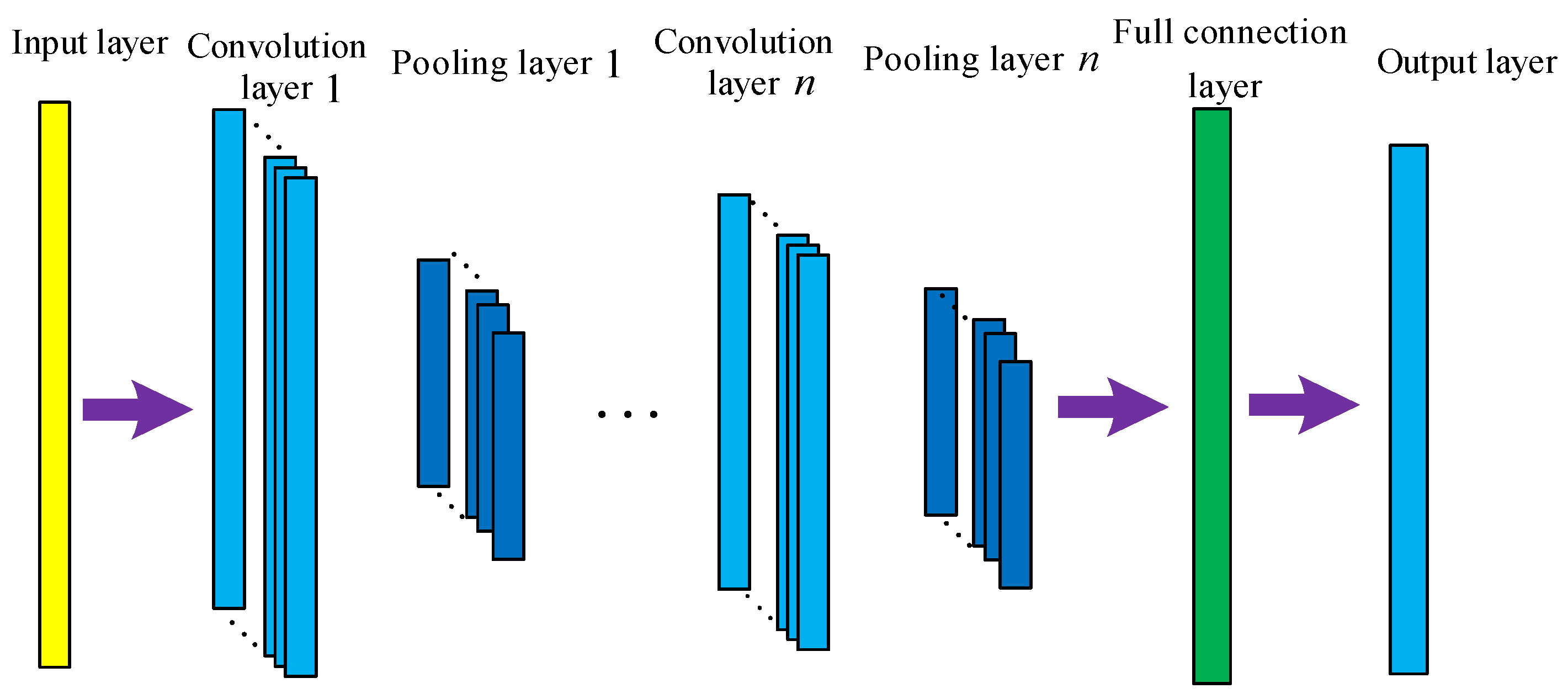
CNN has outstanding spatial feature extraction capabilities, mainly composed of the input layer, convolutional layer, pooling layer, fully connected layer, and output layer, as demonstrated in
Figure 2. The input layer is employed for receiving raw data. The convolutional layer is utilized for extracting features from the input data. The pooling layer downsamples the convolution layer’s output to lower the data’s dimension. The fully connected layer turns the pooling layer’s output into the one-dimensional vector and outputs it through the output layer. Compared with the full connection mode of the traditional neural network, CNN uses a convolution kernel with appropriate size to extract the local features of this layer's input, that is, this CNN convolution layer's neurons are only connected to some upper layer's neurons. This local connectivity method reduces the neural network's parameter count and overfitting risk. At the same time, CNN employs weight sharing to enable convolutional kernels to capture identical features at varying places, resulting in reduced model training complexity and imparting the model with the characteristics of translation invariance. The convolution operation formula is below:
where
represents convolution calculation;
denotes the
-th feature map of the
-th convolution layer;
represents offset;
represents convolution kernel matrix;
represents the nonlinear activation functions;
indicates the number of input feature maps.
3. Hybrid Models
This section describes three combination models, namely the LSTM-ARX model, CNN-ARX model, and LSTM-CNN-ARX model.
3.1. LSTM-ARX Model
LSTM neural network adopts directional circulation, which is better than feedforward neural network to deal with the problem of before and after correlation between data, and is conducive to the establishment of a nonlinear system timing model. Simultaneously, a gating mechanism is introduced in LSTM networks to control the flow and discarding of historical information and input characteristics, which solves the long-term dependence problem in simple RNN networks. In the actual modeling process, single-layer LSTM is usually unable to express complex temporal nonlinear characteristics, so a series approach is often adopted to stack multiple LSTM layers to deepen the network and bolster modeling capabilities. The LSTM-ARX model can be obtained by approximating the function coefficient of the model (3) with LSTM. It combines the benefits of LSTM for handling long sequence data with the SD-ARX model's nonlinear expression capabilities to fully represent the nonlinear system’s dynamic features.
Figure 3 describes the LSTM-ARX model's architecture and its expression below
where
represents output;
represents input;
represents white noise;
,
are model's orders;
denotes time delay;
,
and
represent the model's function coefficient; n denotes the number of hidden layers;
and
represent the hidden layer state and cell state of the
-th hidden layer of time step
at time
;
,
and
represent activation functions (e.g., Hard Sigmoid and Tanh) are employed to improve the model's capability in capturing the system's nonlinearity;
,
and
represent offsets;
,
and
represent weight coefficients.
3.2. CNN-ARX Model
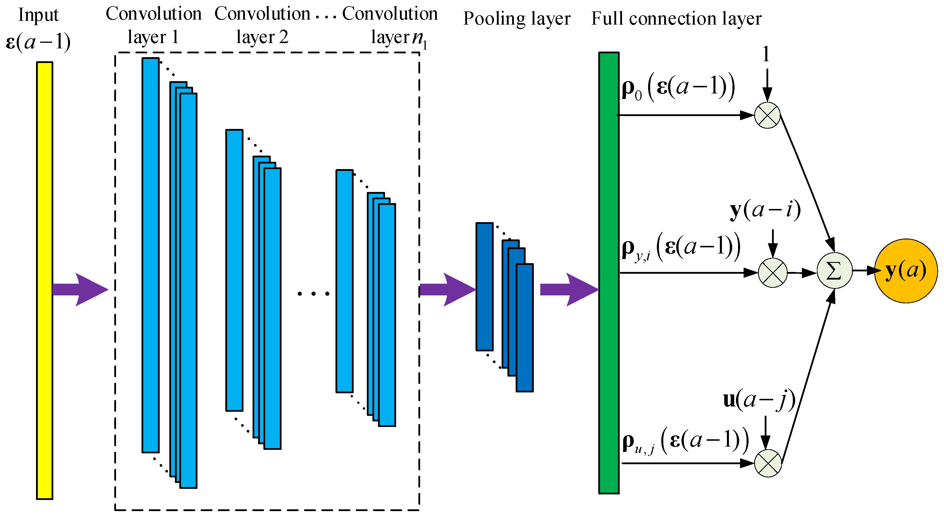
CNN has strong nonlinear feature extraction capabilities. The CNN-ARX model is derived by fitting the SD-ARX model's coefficients by CNN. This model combines the ability of CNN's local feature extraction and the SD-ARX model's expression. Compared to traditional neural networks, CNN has the characteristics of local connection, weight sharing, pooling operation, etc., which can further decrease the complexity and overfitting risks of the model, and enable the model to possess a certain level of robustness and fault tolerance.
Figure 4 describes the CNN-ARX model's architecture and its expression below
where
represents input;
and
represent activation functions;
and
indicates pooling operation and flattening operation;
denotes the one-dimensional vector obtained by flattening the output feature maps
;
,
and
represent weight coefficients;
,
and
represent the offsets.
3.3. LSTM-CNN-ARX Model
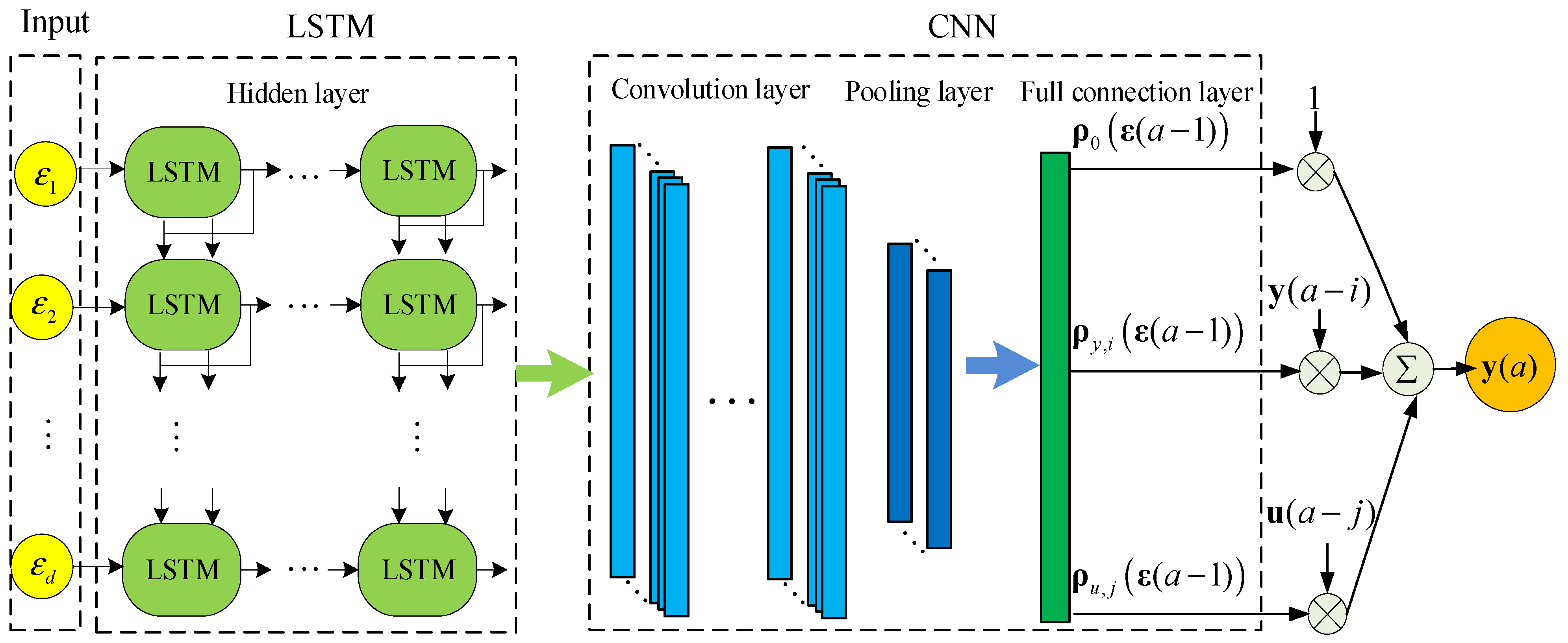
The LSTM-CNN-ARX model is obtained by combining LSTM and CNN to approximate SD-ARX model coefficients, as shown in
Figure 5. First, employ LSTM for learning the temporal characteristics of the input data, followed by the utilization of CNN to capture the spatial characteristics, and finally calculate the SD-ARX model’s correlation coefficients through a full connection layer to obtain the LSTM-CNN-ARX model. This model integrates the spatiotemporal characteristic extraction ability of LSTM-CNN with the expressive power of the SD-ARX model, this approach effectively captures the nonlinear system’s dynamic features. The LSTM-CNN-ARX model's mathematical expression is obtained from Formulas (6) and (7), as follows
The aforementioned deep learning-based SD-ARX models adopt data-driven techniques for modeling. First, select appropriate and effective input and output data as identification data for modeling. Second, based on the complexity of the identified system, select the model’s initial orders, the network's layer count, and the node count per layer. Third, choose activation functions (such as Sigmoid, Tanh, and Relu) and optimizer (such as Adam, and SGD), and configure other hyperparameters of the model. Fourth, train the model and evaluate its performance using a test set, computing the mean square error (MSE). Fifthly, adjust the orders while keeping the other structures of the model unchanged to train the model with new orders again, and select the orders of the model with the minimum MSE as the optimal orders. Next, keep the other structures of the model unchanged, adjust the network's layer count, and select the network's layer count with the smallest MSE as the optimal number of layers. Using the same method, determine the other model structures, i.e., the node count, activation function, and hyperparameters, and ultimately choose the model structure with the smallest MSE as the optimal model.
4. MPC Algorithm Design
This section designs the predictive controller based on models (6)-(8). By utilizing the model's local linear and global nonlinear features, the predictive controller uses current state operating point information to locally linearize the model, calculates the nonlinear system's predicted output, and obtains the control law by solving a quadratic programming (QP) problem.
For the convenience of MPC algorithm development, models (6) - (8) can be converted to the following forms
where
,
and
indicates regression coefficients;
represents the maximum value of
and
;
denotes the white noise.
To transform the above equation into state-space form, design the vectors below
Therefore, Eq. (9) becomes the following form.
where
Note that the coefficient matrix above is related to the working state
at time
. For different state-dependent ARX models, the values of matrices
,
, and
in Equation (12) are different and can be calculated using equation (9). To further develop the model predictive controller, define the vectors below
where
,
,
and
represent the multi-step forward prediction state vector, multi-step forward prediction output vector, multi-step forward prediction control vector, and multi-step forward prediction offset, respectively;
and
represent the
-step forward prediction of the state and output;
and
represent the prediction and control time domains, respectively. The model's multi-step forward prediction control is presented below.
where
In the Formula (14), the coefficient matrices , , , and change with the system state and can be obtained by solving the system's future working point . Nevertheless, in the actual control process, it may be challenging to obtain information on the future state operating point. Therefore, compute using the current operating point instead of for computer. Obtain the locally linearized model according to Equation (11) and use it to develop the following MPC method.
To facilitate the design of the objective function, Equation (14) is converted into the following forms
Then, the desired output
and control increment
are defined
where
. The optimization objective function design for MPC as below
where
;
,
and
represent weight coefficient matrices. Substitute Equations (17) and (18) into Equation (19) to eliminate the constant term and convert it into the following QP problem.
Equation (20) represents a convex QP problem with constraints. If the feasible set defined by the constraint condition is not empty and the objective function has a lower bound within the feasible set, then the QP problem has a globally optimal solution. If Eq. (20) has no feasible solution in a certain control period, the feasible solution obtained in the previous period is used for control in the practical control. In addition, in practical control, in order to avoid control sequence deviations caused by environmental or system inherent biases, the optimal control sequence’s initial value is employed as the control input and observing the system output at the next moment for feedback correction, thus realizing online rolling optimization.
5. Control Experiments
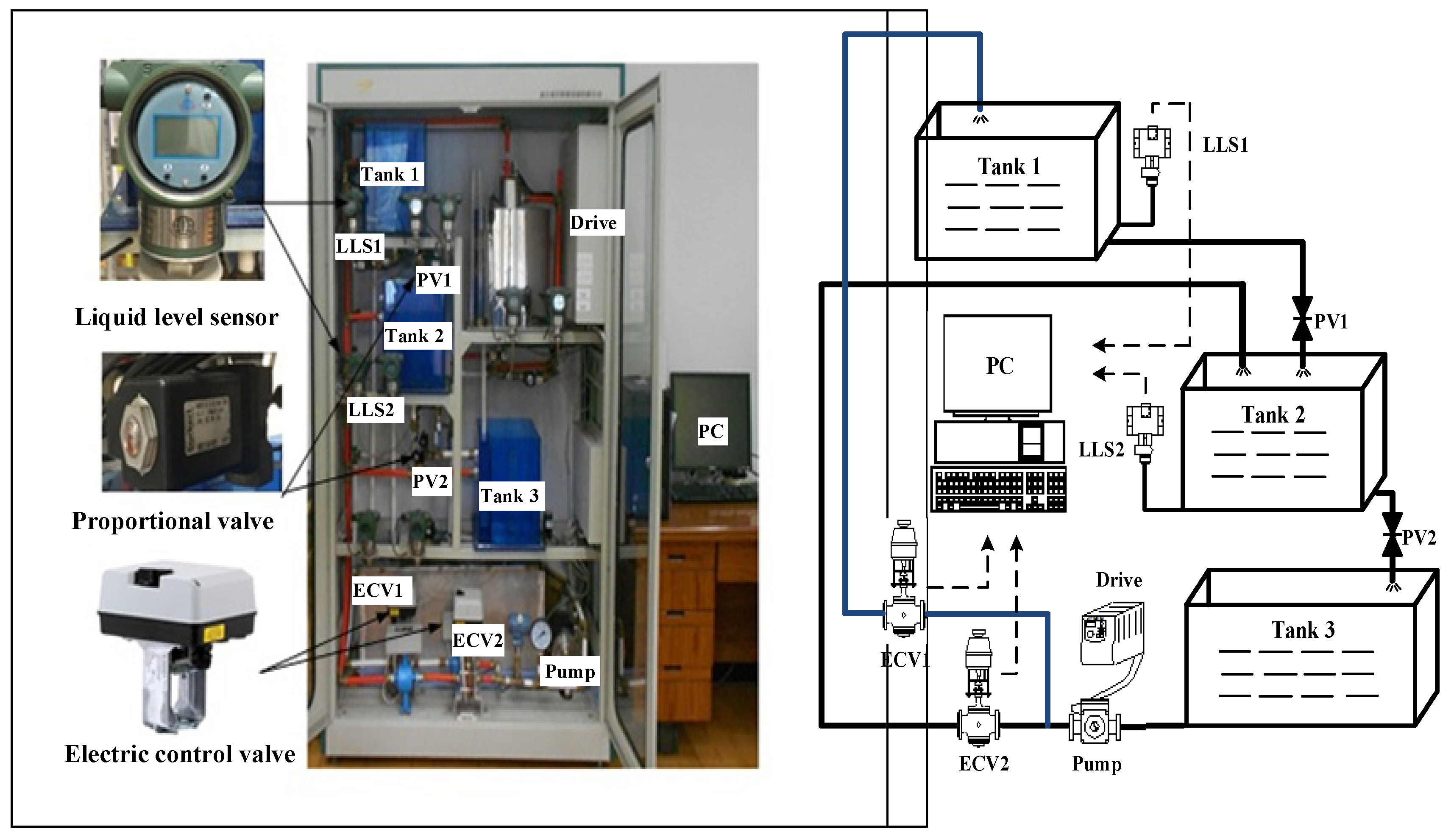
This part uses a water tank system (WTS) shown in
Figure 6 as the experimental object, which is a commonly used process control device in industrial production. The deep learning models are established using the data-driven modeling approach and the predictive controllers are designed based on the model's distinctive structure for real-time control comparative experiments on WTS.
5.1. WTS
WTS is a representative dual-input dual-output process control experimental equipment with strong coupling, large time delay, and strong nonlinearity. The water inflows of water tanks 1 and 2 are controlled by electric control valves ECV1 and ECV2, the water outflows are regulated by proportional valves PV1 and PV2, and the water level heights are detected by the liquid level sensors LLS1 and LLS2. Control experiments were performed on WTS and the models (6)-(8) are designed below:
where
represents the liquid level heights of tank 1 and tank 2;
represents the openings (0%~100%) of electric control valves ECV1 and ECV2;
,
and
are the weight coefficients, which can be obtained by models (6)-(8);
indicates the white noise signal. Among them, we have set the working point
, because the change in water level is an important factor leading to the strongly nonlinear dynamic characteristics of WTS.
5.2. Estimation of Model
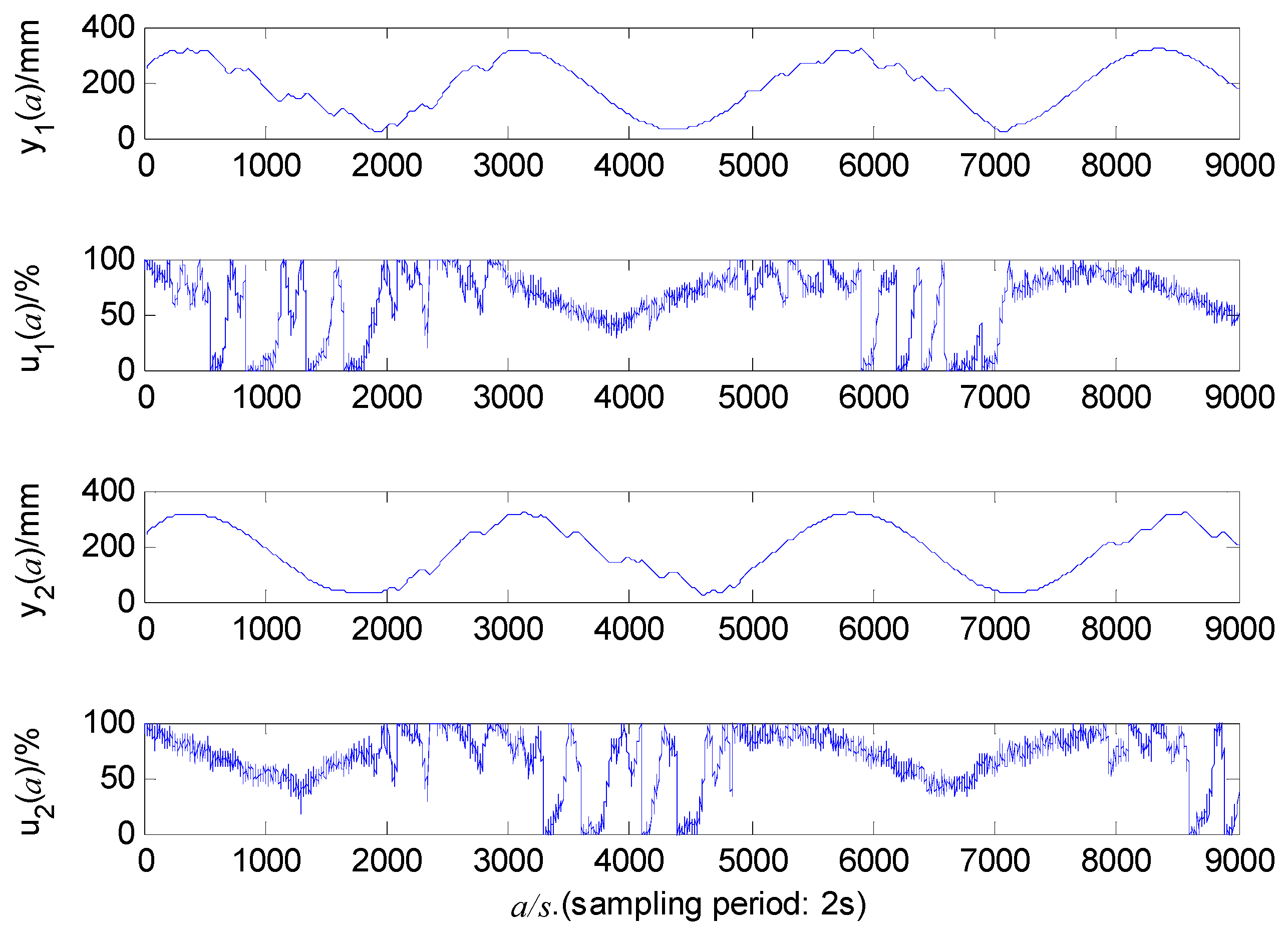
In order to make the collected modeling data contain the various nonlinear dynamic characteristics of the WTS to the maximum extent, this article uses the expected signal including sine and step to control the large fluctuation of the water tank level in the normal working range through the PID controller to obtain effective input/output sampling data. The sampling time is 2 seconds.
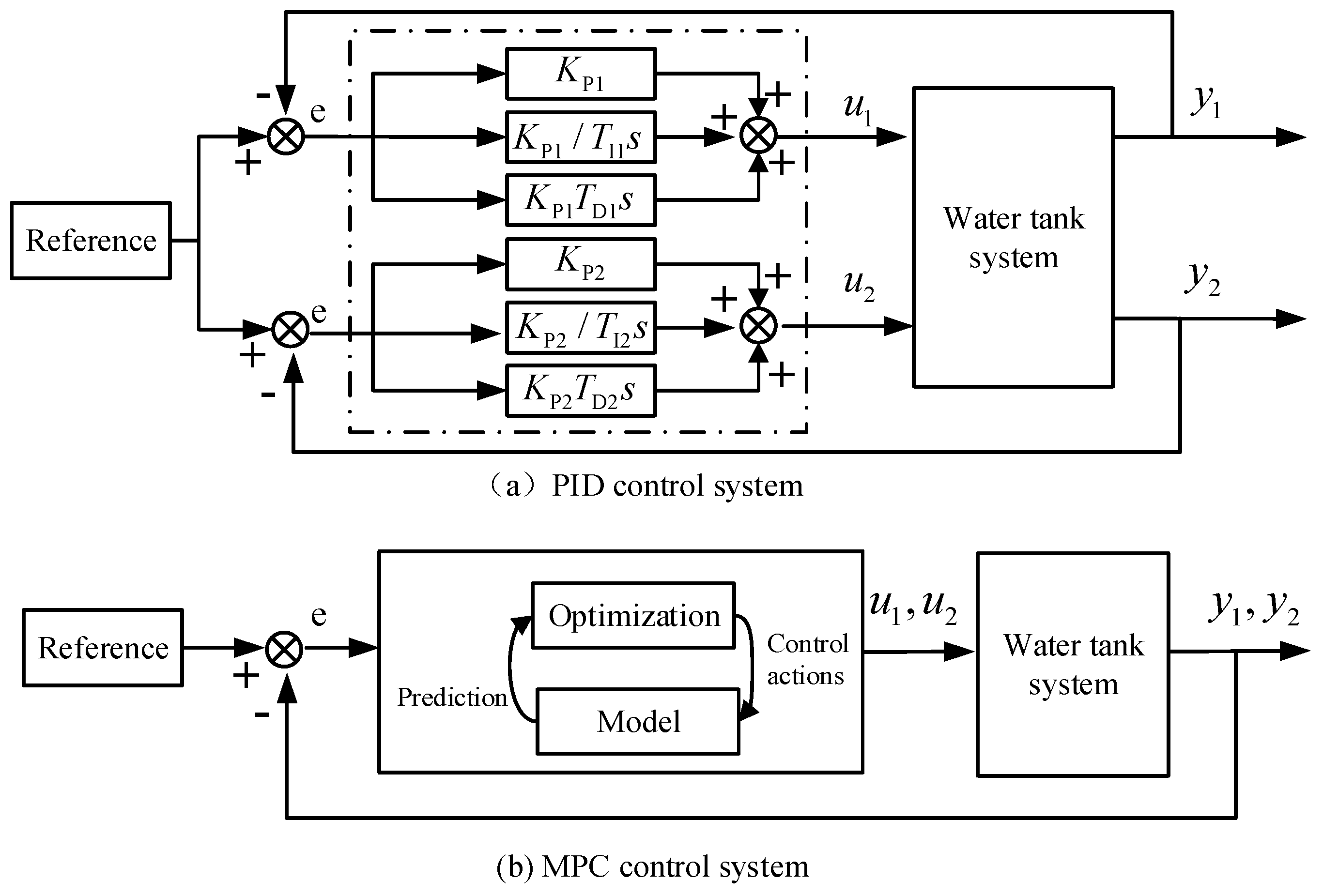
Figure 7 presents the structure of the PID controller used, which is mainly used to generate the system identification data. The PID controller output is limited between 0 and 100 (%).
The sampling data given in
Figure 8 is segregated into different proportions for model training and testing. The best proportion of the final modeling results is that the first 3500 data points (sampling time 2s) are utilized for estimating the model, while the subsequent 1000 data points are utilized for verifying the model.
The parameter optimization algorithms of the deep learning-based SD-ARX models are all the sampling adaptive motion estimation (Adam) algorithm, which integrates the advantages of momentum optimization and adaptive learning rate, with high computational efficiency and can accelerate parameter convergence. Tanh function is the full connecting layer activation function for all models, which gives the models a faster convergence rate and a stronger nonlinear expression ability. The hidden layer activation functions and of the LSTM are the Hard Sigmaid function and Tanh function, respectively. Compared with the standard Sigmoid function, the application of the Hard Sigmaid function in the neural network is more stable. It can reduce the gradient vanishing problem and has a faster calculation speed. The CNN employs the Relu as its convolutional activation function, which assists in reducing redundant calculation and parameter quantity between neurons, thus enhancing the model's efficiency and generalization performance. The CNN pool function selects the average pool, which is beneficial for reducing the model's complexity and minimizing the overfitting risk, and improving the feature’s robustness. Its convolutional and pooling layers have kernel sizes of 3 and 4. The MSE of different model structures is calculated and compared. When the model complexity meets the requirements, select the model structure and parameters with the lowest MSE for real-time control experiments.
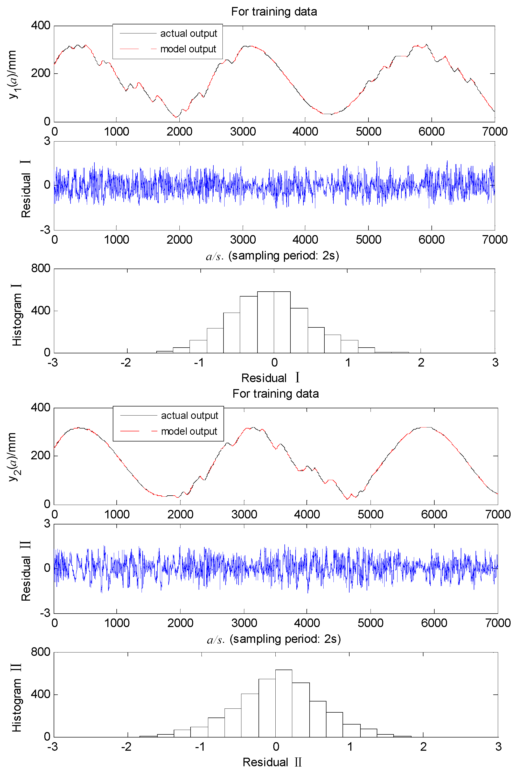
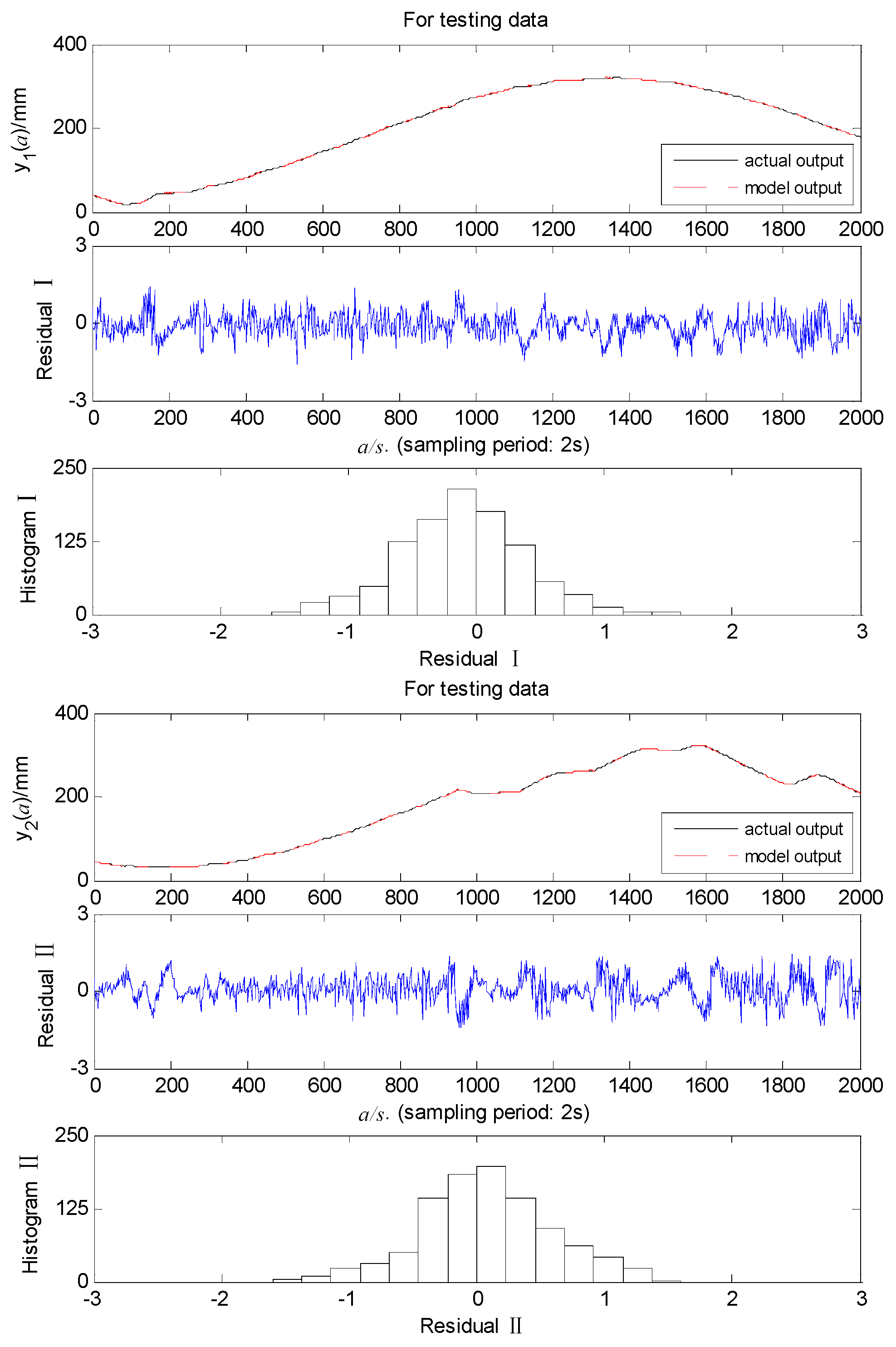
Taking the LSTM-CNN-ARX model as an example,
Figure 9 and
Figure 10 show that the model’s training and testing residuals are very small and the models have high modeling accuracy.
Table 1 illustrates that different models have varying structures because different models have distinct characteristics and nonlinear description capabilities. At the same time, the model with more parameters and deeper network layers has stronger nonlinear expression ability, but this also increases the computational burden, resulting in a longer training time. The findings suggest that the ARX model exhibits the maximum MSE and can not capture the nonlinear system’s dynamic behavior well. The deep learning-based ARX model has lower MSE than the RBF-ARX model because the multi-layer deep learning network has stronger nonlinear expression capabilities than the single-layer RBF neural network. The LSTM-ARX model has less MSE than the CNN-ARX model because LSTM can maintain long-term dependencies on sequence data. In addition, the LSTM-CNN-ARX model incorporating the strengths of LSTM for learning temporal characteristics and CNN for capturing spatial characteristics, its MSE is smaller than the LSTM-ARX and CNN-ARX models, which can accurately capture the WTS’s nonlinear behavior.
5.3. Real-Time Control Experiments
This part presents the WTS’s control experiment in Figure 1, which uses the deep learning ARX model-based MPC method to compare with PID, ARX-MPC, and RBF-ARX-MPC methods, demonstrating the developed method’s superiority. Figure 7 shows the control system’s structure, where the PID controller’s parameters are
and
. Because the WTS operates in different liquid levels, it exhibits varying dynamic behaviors. Thus performing control experiments in different water level regions, i.e., low, medium, and high water level zones. The parameter setting of the objective optimization function (20) for the predictive control method is
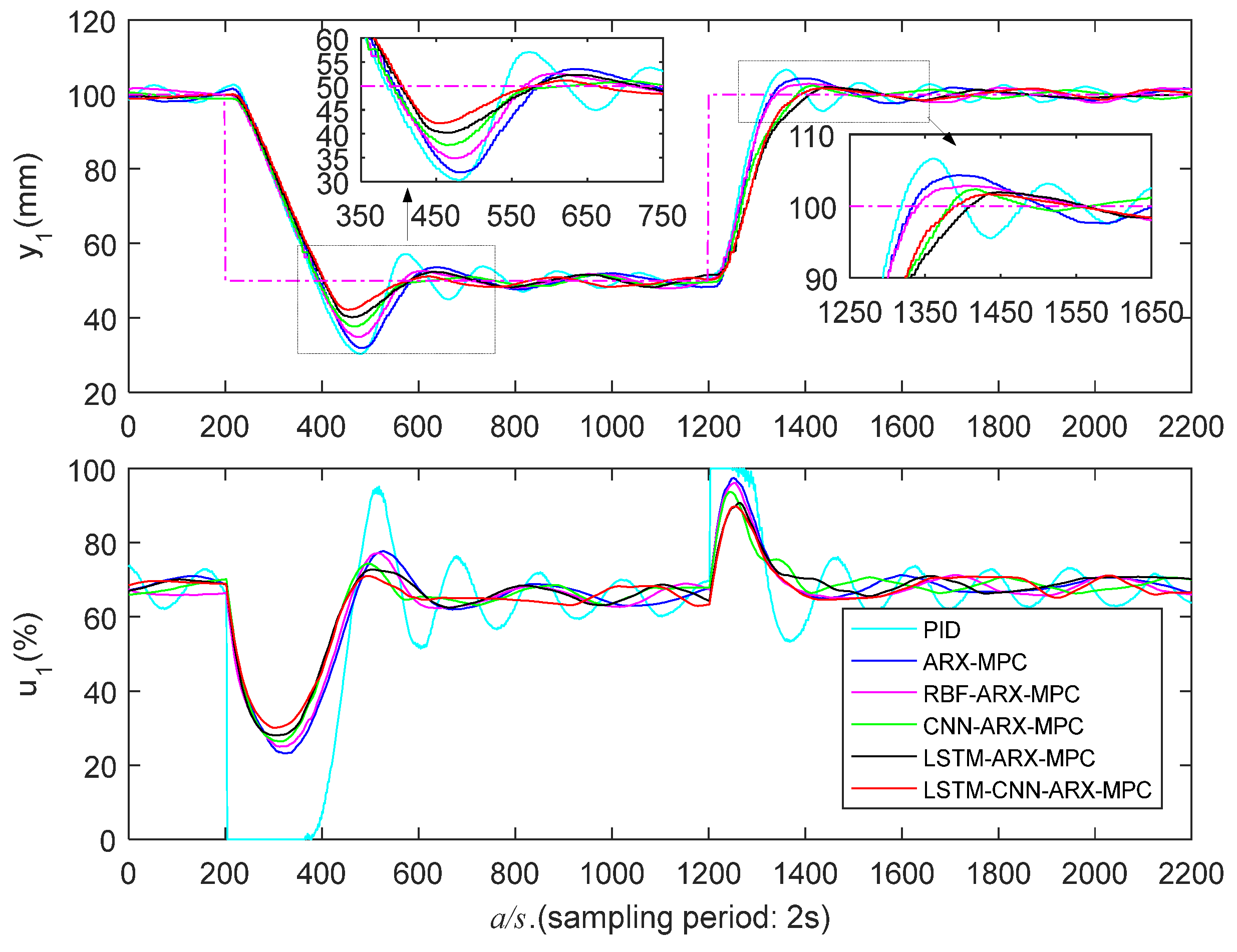
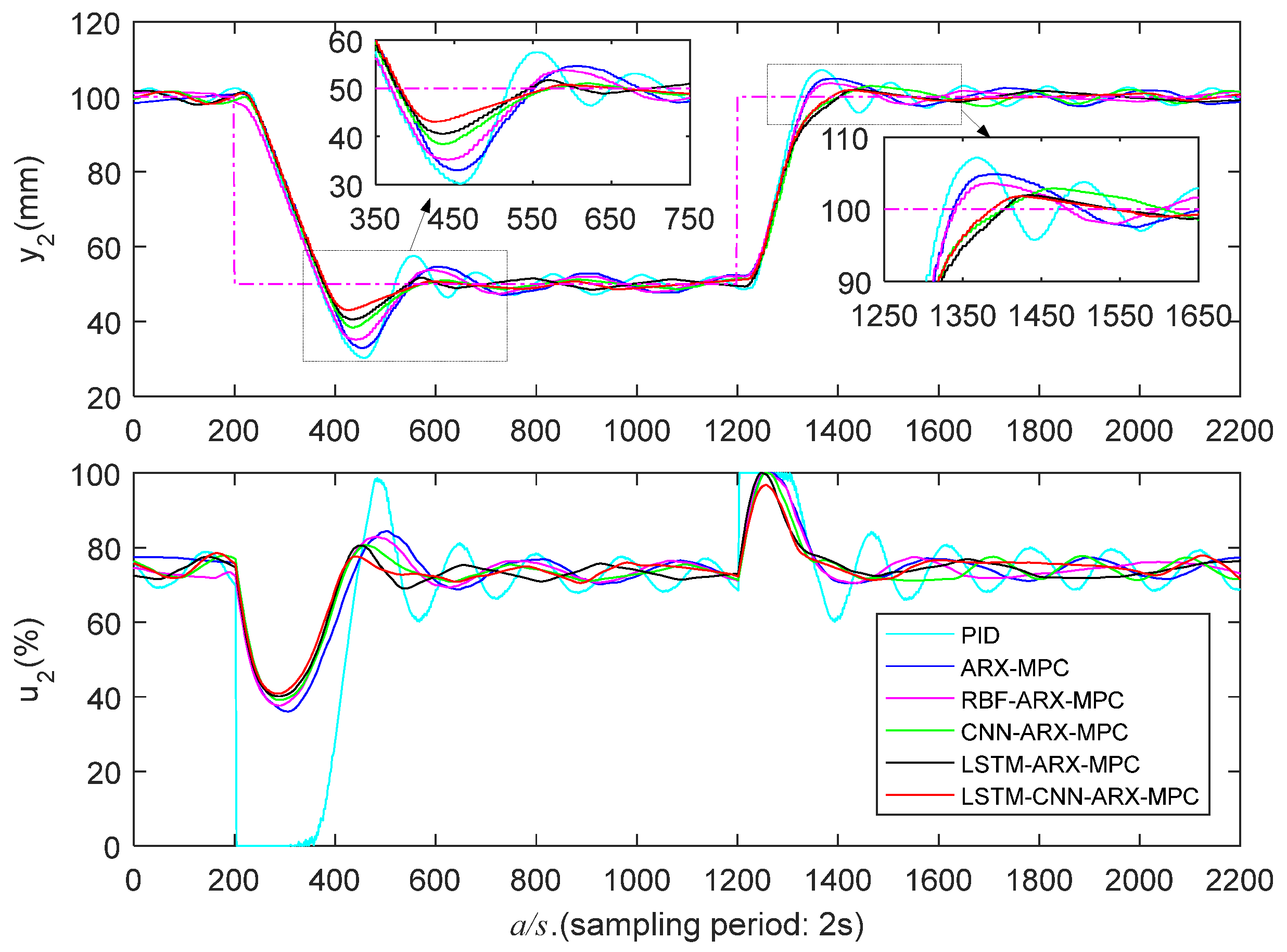
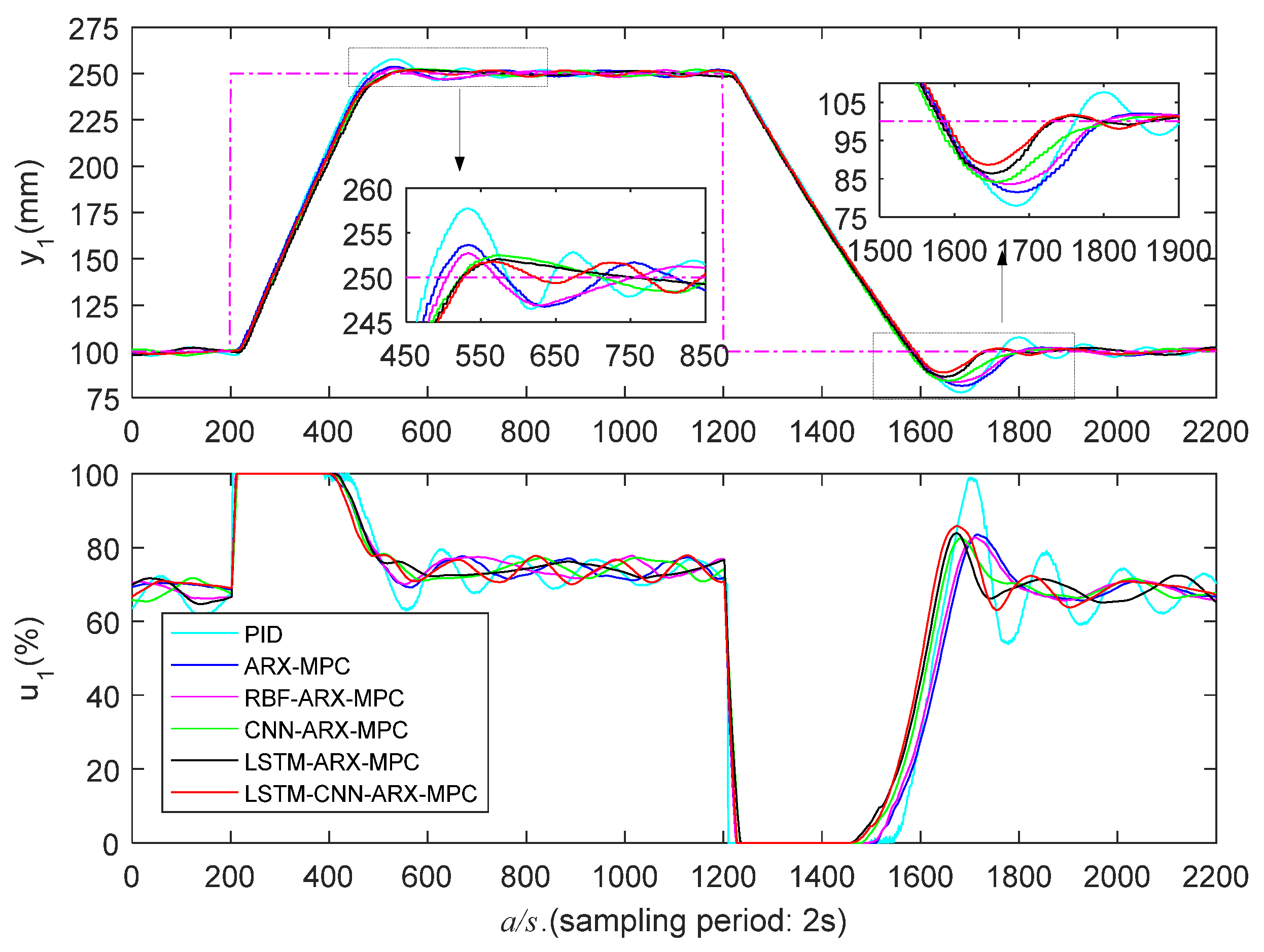
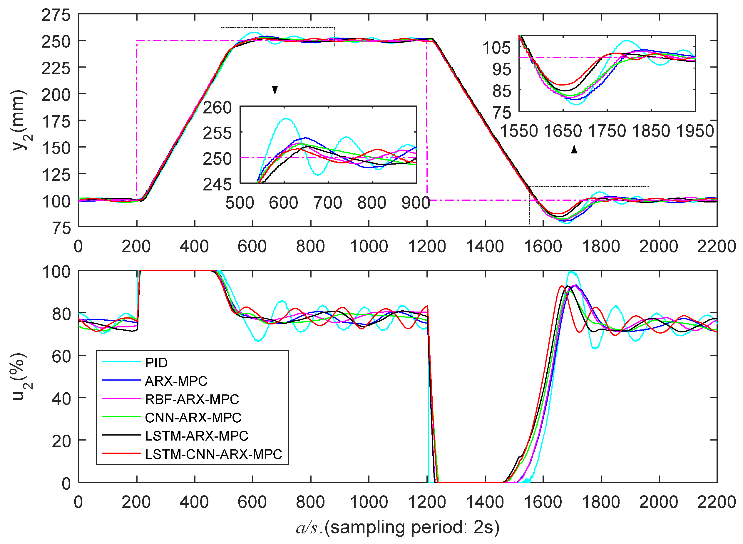
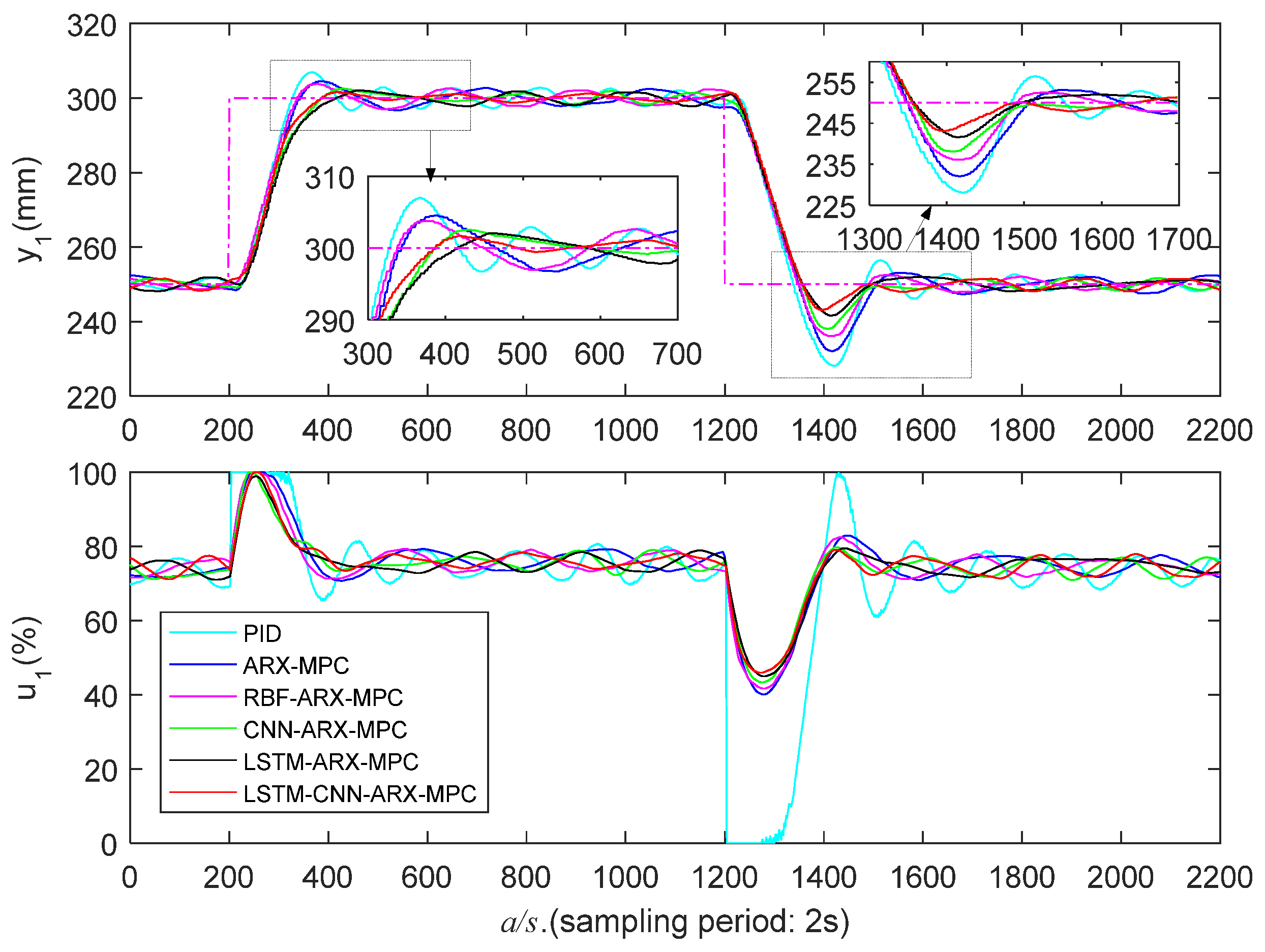
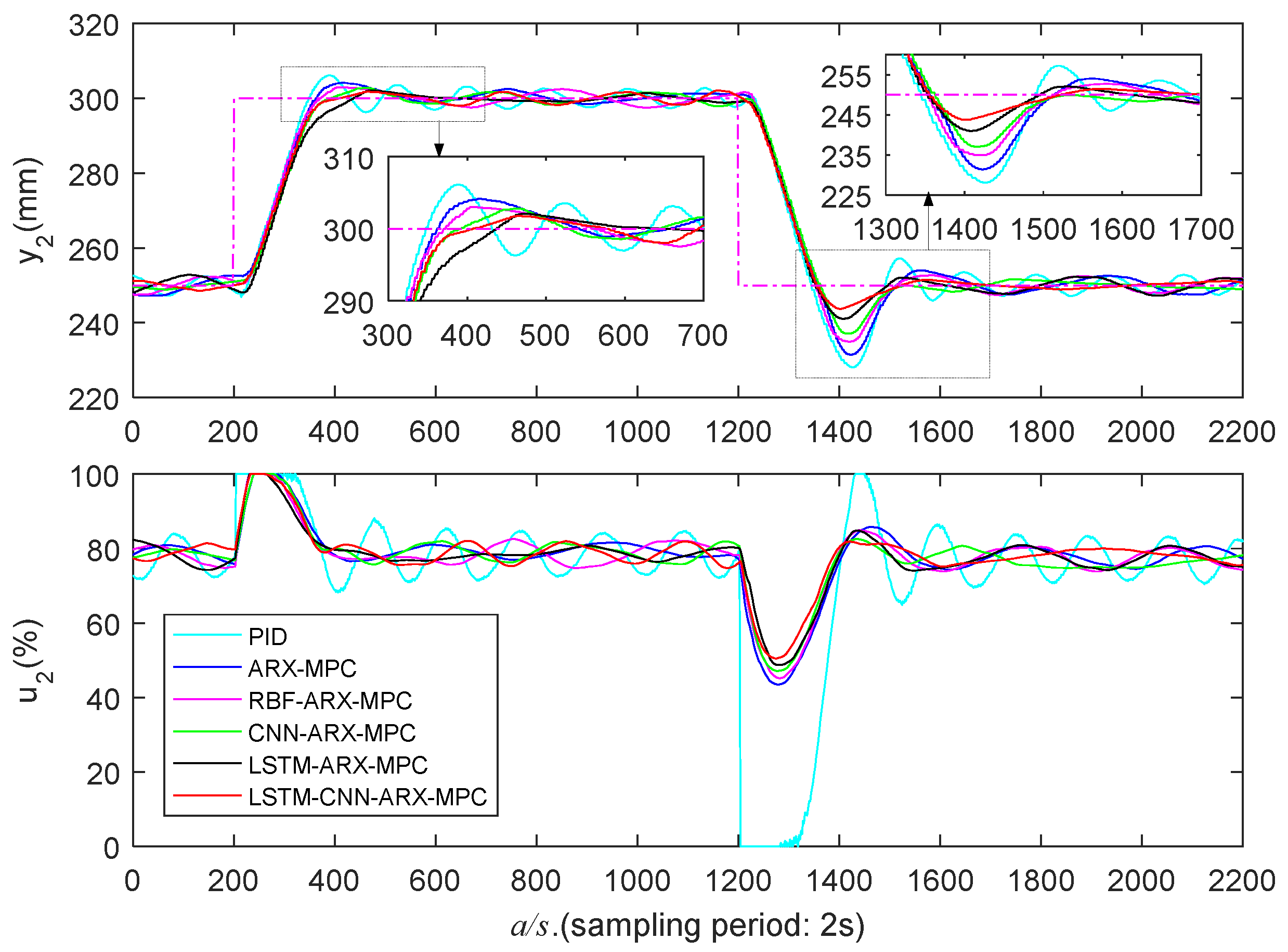
,
,
. The control experimental results of WTS are shown in
Figure 11,
Figure 12,
Figure 13,
Figure 14,
Figure 15 and
Figure 16,where
and
represent the liquid level heights,
and
represent the control valve opening (ranging from 0% to 100%), and
indicates that the expected output is a pink dashed line. In addition,
Table 2,
Table 3 and
Table 4 display each algorithm’s control outcomes, encompassing overshoot (O), peak time (PT), adjustment time (AT),
and
represent the rising and falling step response, respectively.
5.3.1. Low Liquid Level Zone Control Experiments
The control outcomes of distinct algorithms in a low liquid level zone (50-100mm) are presented in
Figure 11 and
Figure 12 and
Table 2, and the LSTM-CNN-ARX-MPC approach shows significantly superior control performance compared to other algorithms. In the falling step response of LSTM-CNN-ARX-MPC, the PTs of liquid level
and
are 252s and 224s, the Os are 15.6% and 14.0%, and the ATs are 336s and 320s; in the rising step response, its Os are 3.2% and 3.6%, and ATs are 166s and 160s, respectively, which are superior to other methods. This is due to the LSTM-CNN-ARX model incorporating the strengths of LSTM for learning temporal characteristics and CNN for capturing spatial characteristics, which can efficiently capture the WTS’s nonlinear characteristics and achieve outstanding control performance. It should be noted that the PT of LSTM-CNN-ARX-MPC may not always outperform other methods. However, the evaluation of control performance is not just about looking at PT, we also need to see other indicators, such as O and AT. In fact, the O and AT of LSTM-CNN-ARX-MPC are much smaller than other methods, so overall, LSTM-CNN-ARX-MPC outperforms other methods. Usually, for controllers, their smaller PT may result in a larger O and AT, and there may also be significant oscillations at the beginning of the control process.
5.3.2. Medium Liquid Level Zone Control Experiments
Figure 13 and
Figure 14 and
Table 3 present the experimental results of various controllers in a medium liquid level zone (100-250 mm), indicating that the PID’s control performance is not as good as other methods, and it has the maximum overshoot and AT. The control effectiveness of RBF-ARX-MPC outperforms ARX-MPC, exhibiting lower O and PT. However, RBF-ARX-MPC demonstrates inferior O and AT compared to the three deep learning-based MPC algorithms. Because multi-layer deep learning networks have stronger nonlinear expression and generalization capabilities than single-layer RBF neural networks, and can adaptively learn the WTS’s nonlinear features. Therefore, the predictive control effect and modeling accuracy based on the deep learning ARX models are better than those of RBF-ARX models. Additionally, the LSTM-ARX-MPC’s comprehensive control effect is marginally superior to CNN-ARX-MPC, because LSTM belongs to a recurrent neural network, which has storage function, and has advantages in time series data modeling, so it can maintain long-term correlation in sequence data. LSTM-CNN-ARX-MPC outperforms all other algorithms in the falling step response, exhibiting the lowest PT, AT, and O. Additionally, it has the smallest O in the rising step response, which enables the WTS’s liquid level to effectively follow the reference trajectory.
5.3.3. High Liquid Level Zone Control Experiments
Figure 15 and
Figure 16 and
Table 4 present the experimental results in a high liquid level zone (250-300 mm). It is apparent that the PID controller exhibits the poorest control performance with the largest O and AT. ARX-MPC's control performance is also poor because the ARX model has limited capability to capture nonlinear features. LSTM-ARX-MPC demonstrates superior overall control performance compared to ARX-MPC, RBF-ARX-MPC, and CNN-ARX-MPC, due to the advantage of LSTM in maintaining long-term dependence on sequence data in time series modeling. LSTM-CNN-ARX-MPC demonstrates the optimal comprehensive control effectiveness, particularly exhibiting considerably lower O in the falling step. This is attributable to the LSTM-CNN-ARX model's powerful spatiotemporal features capturing capability, enabling it to effectively capture the WTS’s nonlinear properties.
In conclusion, PID and ARX-MPC exhibit the poorest control performance, failing to effectively capture the nonlinear characteristics of WTS, thereby limiting their applicability. Additionally, the overall control effectiveness of RBF-ARX-MPC is not as good as deep learning-based MPC. This is because RBF is a single-layer network with lesser nonlinear descriptive capabilities compared to multi-layer deep learning networks. Furthermore, LSTM-ARX-MPC's superior control performance compared to CNN-ARX-MPC can be attributed to LSTM's memory function that preserves the long-term dependence on sequential data. In almost all cases, LSTM-CNN-ARX-MPC demonstrates the best control effectiveness, especially in the low and high water level regions with strong nonlinearity. This is attributed to the powerful spatiotemporal feature learning capability of the LSTM-CNN-ARX model, enabling it to capture all the nonlinear features of WTS.
7. Conclusions
This study aims to solve the modeling and predictive control problem of a category of smooth nonlinear systems. The studied system’s operating point may change over time, and its dynamic characteristics can be locally linearized. We utilized the spatiotemporal feature extraction capabilities of the LSTM and CNN, as well as the SD-ARX model’s pseudo-linear ARX structural feature, to establish the LSTM-CNN-ARX model to describe the studied system’s nonlinear properties. The developed modeling and MPC algorithms were validated in real-time control rather than digital simulation on an actual multivariable water tank system, confirming their effectiveness. The proposed methods can be useful and can generate better results for a category of smooth nonlinear plants than some well-established, simpler, but proven efficiency, approaches.
This article used the deep learning model to fit the state-dependent ARX model’s autoregressive coefficients to obtain the LSTM-ARX model and LSTM-CNN-ARX model that accurately describe the system’s nonlinear properties. These models have local linear and global nonlinear characteristics, which decompose the model’s complexity into the autoregressive part, making it easier to design the MPC controllers. Control comparative experiments demonstrate that compared with the PID, ARX-MPC, and RBF-ARX-MPC algorithms, the three deep learning-based MPC algorithms can achieve more precise trajectory tracking control of the WTS liquid level. This is because of the stronger nonlinear expression and generalization ability of deep learning networks, which can adaptively learn system features and model parameters, and better represent the nonlinear behavior of WTS. Furthermore, the comprehensive control performance of LSTM-CNN-ARX-MPC is superior to LSTM-ARX-MPC and CNN-ARX-MPC due to its incorporating the strengths of LSTM for learning temporal characteristics and CNN for capturing spatial characteristics, which enables it to capture the multi-dimensional spatiotemporal nonlinear features of WTS more effectively.
While LSTM neural networks may effectively address the gradient vanishing or exploding problem in traditional RNN modeling and better handle long sequence data, the complex structure of the LSTM model with numerous unidentified parameters results in significant computational demands during model training, convergence difficulties, and risk of overfitting. Consequently, future studies will concentrate on improving the model structure by replacing the LSTM structure with gated recurrent units or related improved structures to enhance modeling efficiency and expand the model's applicability in scenarios with limited computational resources.
References
- Holkar, K.S.; Waghmare, L.M. An overview of model predictive control. Int. J. Control Autom. Syst. 2010, 3, 47–63. [Google Scholar]
- Elnawawi, S.; Siang, L.C.; O’Connor, D.L.; Gopaluni, R.B. Interactive visualization for diagnosis of industrial Model Predictive Controllers with steady-state optimizers. Control Eng. Practice 2022, 121, 105056. [Google Scholar] [CrossRef]
- Kwapień, J.; Drożdż, S. Physical approach to complex systems. Phys. Rep.-Rev. Sec. Phys. Lett. 2012, 515, 115–226. [Google Scholar] [CrossRef]
- Chen, H.; Jiang, B.; Ding, S.X.; Huang, B. Data-driven fault diagnosis for traction systems in high-speed trains: A survey, challenges, and perspectives. IEEE Trans. Intell. Transp. Syst. 2022, 23, 1700–1716. [Google Scholar] [CrossRef]
- Yu, W.; Wu, M.; Huang, B.; Lu, C. A generalized probabilistic monitoring model with both random and sequential data. Automatica 2022, 144, 110468. [Google Scholar] [CrossRef]
- Pareek, P.; Verma, A. Piecewise Linearization of Quadratic Branch Flow Limits by Irregular Polygon. IEEE Trans. Power Syst. 2018, 33, 7301–7304. [Google Scholar] [CrossRef]
- Ławryńczuk, M. Nonlinear predictive control of a boiler-turbine unit: A state-space approach with successive on-line model linearisation and quadratic optimisation. ISA Trans. 2017, 67, 476–495. [Google Scholar] [CrossRef] [PubMed]
- Qian, K.; Zhang, Y. Bilinear model predictive control of plasma keyhole pipe welding process. J. Manuf. Sci. Eng.-Trans. ASME 2014, 136, 31002. [Google Scholar] [CrossRef]
- Nie, Z.; Gao, F.; Yan, C.B. A multi-timescale bilinear model for optimization and control of HVAC systems with consistency. Energies 2021, 14, 400. [Google Scholar] [CrossRef]
- Shi, Y.; Yu, D.L.; Tian, Y.; Shi, Y. Air-fuel ratio prediction and NMPC for SI engines with modified Volterra model and RBF network. Eng. Appl. Artif. Intell. 2015, 45, 313–324. [Google Scholar] [CrossRef]
- Gruber, J.K.; Ramirez, D.R.; Limon, D.; Alamo, T. A convex approach for NMPC based on second order Volterra series models. Int. J. Robust Nonlinear Control 2015, 25, 3546–3571. [Google Scholar] [CrossRef]
- Chen, H.; Chen, Z.; Chai, Z.; Jiang, B.; Huang, B. A single-side neural network-aided canonical correlation analysis with applications to fault diagnosis. IEEE T. Cybern. 2021, 52, 9454–9466. [Google Scholar] [CrossRef]
- Chen, H.; Liu, Z.; Alippi, C.; Huang, B.; Liu, D. Explainable intelligent fault diagnosis for nonlinear dynamic systems: From unsupervised to supervised learning. IEEE Trans. Neural Netw. Learn. Syst. 2022. [Google Scholar] [CrossRef] [PubMed]
- Ding, B.; Wang, J.; Su, B. Output feedback model predictive control for Hammerstein model with bounded disturbance. IET Contr. Theory Appl. 2022, 16, 1032–1041. [Google Scholar] [CrossRef]
- [15] Raninga, D.; TK, R.; Velswamy, K. Explicit nonlinear predictive control algorithms for Laguerre filter and sparse least square support vector machine-based Wiener model. Trans. Inst. Meas. Control 2021, 43, 812–831. [Google Scholar] [CrossRef]
- Wang, Z.; Georgakis, C. Identification of Hammerstein-Weiner models for nonlinear MPC from infrequent measurements in batch processes. J. Process Control 2019, 82, 58–69. [Google Scholar] [CrossRef]
- Du, J.; Zhang, L.; Chen, J.; Li, J.; Zhu, C. Multi-model predictive control of Hammerstein-Wiener systems based on balanced multi-model partition. Math. Comput. Model. Dyn. Syst. 2019, 25, 333–353. [Google Scholar] [CrossRef]
- Peng, H.; Ozaki, T.; Haggan-Ozaki, V.; Toyoda, Y. A parameter optimization method for radial basis function type models. IEEE Trans. Neural Netw. 2003, 14, 432–438. [Google Scholar] [CrossRef] [PubMed]
- Zhou, F.; Peng, H.; Qin, Y.; Zeng, X.; Xie, W.; Wu, J. RBF-ARX model-based MPC strategies with application to a water tank system. J. Process Contr 2015, 34, 97–116. [Google Scholar] [CrossRef]
- Peng, H.; Nakano, K.; Shioya, H. Nonlinear predictive control using neural nets-based local linearization ARX model—Stability and industrial application. IEEE Trans. Control Syst. Technol. 2006, 15, 130–143. [Google Scholar] [CrossRef]
- Kang, T.; Peng, H.; Zhou, F.; Tian, X.; Peng, X. Robust predictive control of coupled water tank plant. Appl. Intell. 2021, 51, 5726–5744. [Google Scholar] [CrossRef]
- Tian, X.; Peng, H.; Zeng, X.; Zhou, F.; Xu, W.; Peng, X. A modelling and predictive control approach to linear two-stage inverted pendulum based on RBF-ARX model. Int. J. Control 2021, 94, 351–369. [Google Scholar] [CrossRef]
- Peng, H.; Wu, J.; Inoussa, G.; Deng, Q.; Nakano, K. Nonlinear system modeling and predictive control using the RBF nets-based quasi-linear ARX model. Control Eng. Practice 2009, 17, 59–66. [Google Scholar] [CrossRef]
- Xu, W.; Peng, H.; Tian, X.; Peng, X. DBN based SD-ARX model for nonlinear time series prediction and analysis. Appl. Intell. 2020, 50, 4586–4601. [Google Scholar] [CrossRef]
- Inoussa, G.; Peng, H.; Wu, J. Nonlinear time series modeling and prediction using functional weights wavelet neural network-based state-dependent AR model. Neurocomputing 2012, 86, 59–74. [Google Scholar] [CrossRef]
- Mu, R.; Zeng, X. A review of deep learning research. KSII Trans. Internet Inf. Syst. 2019, 13, 1738–1764. [Google Scholar] [CrossRef]
- Lippi, M.; Montemurro, M.A.; Degli Esposti, M.; Cristadoro, G. Natural language statistical features of LSTM-generated texts. IEEE Trans. Neural Netw. Learn. Syst. 2019, 30, 3326–3337. [Google Scholar] [CrossRef]
- Tayal, A.R; Tayal, M.A. DARNN: Discourse Analysis for Natural languages using RNN and LSTM. Int. J. Next-Gener. Comput. 2021, 12, 762–770. [Google Scholar] [CrossRef]
- Shuang, K.; Li, R.; Gu, M. , Loo, J.; Su, S. Major-minor long short-term memory for word-level language model. IEEE Trans. Neural Netw. Learn. Syst. 2019, 31, 3932–3946. [Google Scholar] [CrossRef]
- Ying, W.; Zhang, L.; Deng, H. Sichuan dialect speech recognition with deep LSTM network. Front.. Comput. Sci. 2020, 14, 378–387. [Google Scholar] [CrossRef]
- Jo, J.; Kung, J.; Lee, Y. Approximate LSTM computing for energy-efficient speech recognition. Electronics 2020, 9, 2004. [Google Scholar] [CrossRef]
- Oruh, J.; Viriri, S.; Adegun, A. Long short-term Memory Recurrent neural network for Automatic speech recognition. IEEE Access 2022, 10, 30069–30079. [Google Scholar] [CrossRef]
- Yang, B.; Yin, K.; Lacasse, S.; Liu, Z. Time series analysis and long short-term memory neural network to predict landslide displacement. Landslides 2019, 16, 677–694. [Google Scholar] [CrossRef]
- Hu, J.; Wang, X.; Zhang, Y.; Zhang, D.; Zhang, M.; Xue, J. Time series prediction method based on variant LSTM recurrent neural network. Neural Process. Lett. 2020, 52, 1485–1500. [Google Scholar] [CrossRef]
- Peng, L.; Zhu, Q.; Lv, S. X.; Wang, L. Effective long short-term memory with fruit fly optimization algorithm for time series forecasting. Soft Comput. 2020, 24, 15059–15079. [Google Scholar] [CrossRef]
- Langeroudi, M.K.; Yamaghani, M.R.; Khodaparast, S. FD-LSTM: A Fuzzy LSTM Model for Chaotic Time-Series Prediction. IEEE Intell. Syst. 2022, 37, 70–78. [Google Scholar] [CrossRef]
- Wu, Z.; Rincon, D.; Luo, J.; Christofides, P.D. Machine learning modeling and predictive control of nonlinear processes using noisy data. AICHE J. 2021, 67, e17164. [Google Scholar] [CrossRef]
- Terzi, E.; Bonassi, F.; Farina, M.; Scattolini, R. Learning model predictive control with long short-term memory networks. Int. J. Robust Nonlinear Control 2021, 31, 8877–8896. [Google Scholar] [CrossRef]
- Zarzycki, K.; Ławryńczuk, M. Advanced predictive control for GRU and LSTM networks. Inf. Sci. 2022, 616, 229–254. [Google Scholar] [CrossRef]
- Yu, W.; Zhao, C.; Huang, B. MoniNet with concurrent analytics of temporal and spatial information for fault detection in industrial processes. IEEE T. Cybern. 2021, 52, 8340–8351. [Google Scholar] [CrossRef]
- Li, G.; Huang, Y.; Chen, Z.; Chesser, G.D.; Purswell, J.L.; Linhoss, J.; Zhao, Y. Practices and applications of convolutional neural network-based computer vision systems in animal farming: A review. Sensors 2021, 21, 1492. [Google Scholar] [CrossRef]
- Yang, X.; Ye, Y.; Li, X.; Lau, R.Y.; Zhang, X.; Huang, X. Hyperspectral image classification with deep learning models. IEEE Trans. Geosci. Remote Sensing 2018, 56, 5408–5423. [Google Scholar] [CrossRef]
- Gu, J.; Wang, Z.; Kuen, J.; Ma, L.; Shahroudy, A.; Shuai, B.; Chen, T. Recent advances in convolutional neural networks. Pattern Recognit. 2018, 77, 354–377. [Google Scholar] [CrossRef]
- Jiang, M.; Zhang, W.; Zhang, M.; Wu, J.; Wen, T. An LSTM-CNN attention approach for aspect-level sentiment classification. J. Comput. Methods Sci. Eng. 2019, 19, 859–868. [Google Scholar] [CrossRef]
- Senthil Kumar, B.; Malarvizhi, N. Bi-directional LSTM-CNN combined method for sentiment analysis in part of speech tagging (PoS). Int. J. Speech Technol. 2020, 23, 373–380. [Google Scholar] [CrossRef]
- Priyadarshini, I.; Cotton, C. A novel LSTM-CNN-grid search-based deep neural network for sentiment analysis. J. Supercomput. 2021, 77, 13911–13932. [Google Scholar] [CrossRef]
- Jang, B.; Kim, M.; Harerimana, G.; Kang, S.U.; Kim, J.W. Bi-LSTM model to increase accuracy in text classification: Combining Word2vec CNN and attention mechanism. Appl. Sci.-Basel 2020, 10, 5841. [Google Scholar] [CrossRef]
- Shrivastava, G. K.; Pateriya, R. K.; Kaushik, P. An efficient focused crawler using LSTM-CNN based deep learning. Int. J. Syst. Assur. Eng. Manag. 2022, 14, 391–407. [Google Scholar] [CrossRef]
- Zhu, Y.; Gao, X.; Zhang, W.; Liu, S.; Zhang, Y. A bi-directional LSTM-CNN model with attention for aspect-level text classification. Future Internet 2018, 10, 116. [Google Scholar] [CrossRef]
Figure 1.
The schematic diagram of LSTM.
Figure 1.
The schematic diagram of LSTM.
Figure 2.
The CNN's framework.
Figure 2.
The CNN's framework.
Figure 3.
The LSTM-ARX model's architecture.
Figure 3.
The LSTM-ARX model's architecture.
Figure 4.
The CNN-ARX model's architecture.
Figure 4.
The CNN-ARX model's architecture.
Figure 5.
The LSTM-CNN-ARX model's architecture.
Figure 5.
The LSTM-CNN-ARX model's architecture.
Figure 6.
Water tank system.
Figure 6.
Water tank system.
Figure 7.
The structure of MPC and PID control systems.
Figure 7.
The structure of MPC and PID control systems.
Figure 8.
Identification data of WTS.
Figure 8.
Identification data of WTS.
Figure 9.
LSTM-CNN-ARX model’s training result.
Figure 9.
LSTM-CNN-ARX model’s training result.
Figure 10.
LSTM-CNN-ARX model’s testing result.
Figure 10.
LSTM-CNN-ARX model’s testing result.
Figure 11.
Low liquid level zone’s experimental results (/).
Figure 11.
Low liquid level zone’s experimental results (/).
Figure 12.
Low liquid level zone’s experimental results (/).
Figure 12.
Low liquid level zone’s experimental results (/).
Figure 13.
Medium liquid level zone’s experimental results (/).
Figure 13.
Medium liquid level zone’s experimental results (/).
Figure 14.
Medium liquid level zone’s experimental results (/).
Figure 14.
Medium liquid level zone’s experimental results (/).
Figure 15.
High liquid level zone’s experimental results (/).
Figure 15.
High liquid level zone’s experimental results (/).
Figure 16.
High liquid level zone’s experimental results (/).
Figure 16.
High liquid level zone’s experimental results (/).
Table 1.
Comparison of modeling results.
Table 1.
Comparison of modeling results.
| Models |
Number of nodes in each layer |
Number of parameters |
Training time |
MSE of training data
|
MSE of testing data
|
| ARX(18,18,6,/,/,/) |
/ |
74 |
18s |
0.4910 |
0.3526 |
0.4176 |
0.4101 |
| RBF-ARX(23,20,6,2,/,/) |
2 |
562 |
169s |
0.4525 |
0.3158 |
0.3804 |
0.3712 |
| CNN-ARX(19,22,6,2,0,3) |
8,16,8 |
3142 |
205s |
0.4277 |
0.2925 |
0.3562 |
0.3448 |
| LSTM-ARX(18,20,6,2,3,0) |
16,32,16 |
23738 |
1152s |
0.4013 |
0.2634 |
0.3353 |
0.3163 |
| LSTM-CNN-ARX(22,21,6,2,3,3) |
8,8,8,16,16,16 |
9710 |
1160s |
0.3732 |
0.2437 |
0.3076 |
0.2866 |
Table 2.
Low liquid level zone’s control performance.
Table 2.
Low liquid level zone’s control performance.
| Control strategy |
|
|
| PT (s) |
O (%) |
AT (s) |
PT (s) |
O (%) |
AT (s) |
|
/
|
/
|
/
|
/
|
/
|
/
|
| PID |
280/162 |
39.4/13.3 |
692/616 |
258/170 |
39.5/14.2 |
814/782 |
| ARX-MPC |
278/194 |
36.2/8.6 |
478/256 |
256/194 |
34.2/9.6 |
732/376 |
| RBF-ARX-MPC |
272/208 |
30.2/5.6 |
420/242 |
242/186 |
29.6/7.2 |
534/234 |
| CNN-ARX-MPC |
264/218 |
25.0/4.6 |
352/172 |
240/268 |
23.2/5.8 |
340/248 |
| LSTM-ARX-MPC |
262/248 |
19.6/3.8 |
348/186 |
236/238 |
19.0/4.0 |
326/184 |
| LSTM-CNN-ARX-MPC |
252/234 |
15.6/3.2 |
336/166 |
224/222 |
14.0/3.6 |
320/160 |
Table 3.
Medium liquid level zone’s control performance.
Table 3.
Medium liquid level zone’s control performance.
| Control strategy |
|
|
| PT (s) |
O (%) |
AT (s) |
PT (s) |
O (%) |
AT (s) |
|
/
|
/
|
/
|
/
|
/
|
/
|
| PID |
332/486 |
5.1/14.7 |
342/606 |
404/480 |
5.0/14.3 |
414/604 |
| ARX-MPC |
336/484 |
2.4/12.4 |
268/566 |
448/476 |
2.5/13.1 |
330/558 |
| RBF-ARX-MPC |
334/474 |
1.8/11.0 |
280/552 |
436/466 |
1.8/12.4 |
334/548 |
| CNN-ARX-MPC |
374/456 |
1.7/10.6 |
276/528 |
440/466 |
1.7/11.8 |
332/546 |
| LSTM-ARX-MPC |
372/450 |
1.3/9.1 |
278/502 |
454/454 |
1.4/10.3 |
328/512 |
| LSTM-CNN-ARX-MPC |
366/444 |
1.1/7.5 |
274/490 |
430/448 |
1.1/8.5 |
326/502 |
Table 4.
High liquid level zone’s control performance.
Table 4.
High liquid level zone’s control performance.
| Control strategy |
|
|
| PT (s) |
O (%) |
AT (s) |
PT (s) |
O (%) |
AT (s) |
|
/
|
/
|
/
|
/
|
/
|
/
|
| PID |
168/222 |
14.0/44.0 |
776/726 |
190/228 |
12.3/43.8 |
942/958 |
| ARX-MPC |
188/218 |
9.0/36.0 |
532/498 |
216/226 |
8.2/37.2 |
546/748 |
| RBF-ARX-MPC |
176/214 |
7.4/28.4 |
456/330 |
206/220 |
6.0/30.0 |
322/526 |
| CNN-ARX-MPC |
230/210 |
5.0/23.6 |
236/282 |
262/216 |
5.6/26.0 |
280/294 |
| LSTM-ARX-MPC |
258/214 |
4.0/16.8 |
184/272 |
272/208 |
4.2/18.0 |
206/278 |
| LSTM-CNN-ARX-MPC |
216/196 |
3.2/13.8 |
162/260 |
266/202 |
3.6/12.6 |
164/272 |
|
Disclaimer/Publisher’s Note: The statements, opinions and data contained in all publications are solely those of the individual author(s) and contributor(s) and not of MDPI and/or the editor(s). MDPI and/or the editor(s) disclaim responsibility for any injury to people or property resulting from any ideas, methods, instructions or products referred to in the content. |
© 2023 by the authors. Licensee MDPI, Basel, Switzerland. This article is an open access article distributed under the terms and conditions of the Creative Commons Attribution (CC BY) license (http://creativecommons.org/licenses/by/4.0/).
