Preprint
Article

On the Development of a Digital Twin for Underwater UXO Detection Using Magnetometer-Based Data in Application for the Training Set Generation for Machine Learning Models

Altmetrics

Downloads

84

Views

37

Comments

0

A peer-reviewed article of this preprint also exists.

Submitted:

02 June 2023

Posted:

02 June 2023

You are already at the latest version

Alerts
Abstract
Scanning underwater areas, using magnetometers, in search of unexploded ordnance is a difficult challenge, where machine learning methods can find a significant application. However, this requires the creation of a set enabling the training of prediction models. Such a task is difficult and costly due to the limited availability of relevant data. To meet this challenge in the article, we propose the use of numerical modeling to solve this task. The conducted experiments allow us to conclude that it is possible to obtain high compliance of the numerical model with the results of physical tests. In addition, the paper discusses the methodology of simplifying the computational model, allowing for almost three times reduction of the calculation time. In addition, in the work we present the methodology of creating an appropriate data set, enabling the generation of any number of training samples.
Keywords: 
Subject: Engineering  -   Safety, Risk, Reliability and Quality

1. Introduction

In the world, and especially in the geographical area of Europe, the problem of munitions, chemical weapons, and shipwrecks with fuel in tanks dumped in water reservoirs is becoming an increasingly urgent problem to solve. Particularly after World War II, munitions and chemical weapons remaining after the war, which various countries wanted to get rid of in the cheapest possible way, were sunk in masse. It is estimated that in the Baltic Sea there may be at least 40 thousand tons of the war remnants mentioned above [1]. Although two main areas for dumping weapons were selected, the Gotland Deep and the Bornholm Deep, a significant part of the weapons was dumped in unidentified places. Currently, due to progressing corrosion, threatening unsealing of weapons and release of poisonous substances into the environment, and the intensive installation works carried out in maritime areas, they force the development of effective and efficient methods to identify dangerous objects.
The task of searching for dangerous objects in the aquatic environment, in particular unexploded ordnance (UXO), requires scanning the surveyed area with various types of sensors (magnetometers, sonars, video cameras, although in this article we focus only on magnetometers). In the next step, specialists analyze the collected data and mark places containing potentially dangerous objects. These sites are subject to further inspection or extraction work carried out by sapper divers. Their work is very expensive because of the limited number of such experts, as well as the limited time possible to spend under the water.
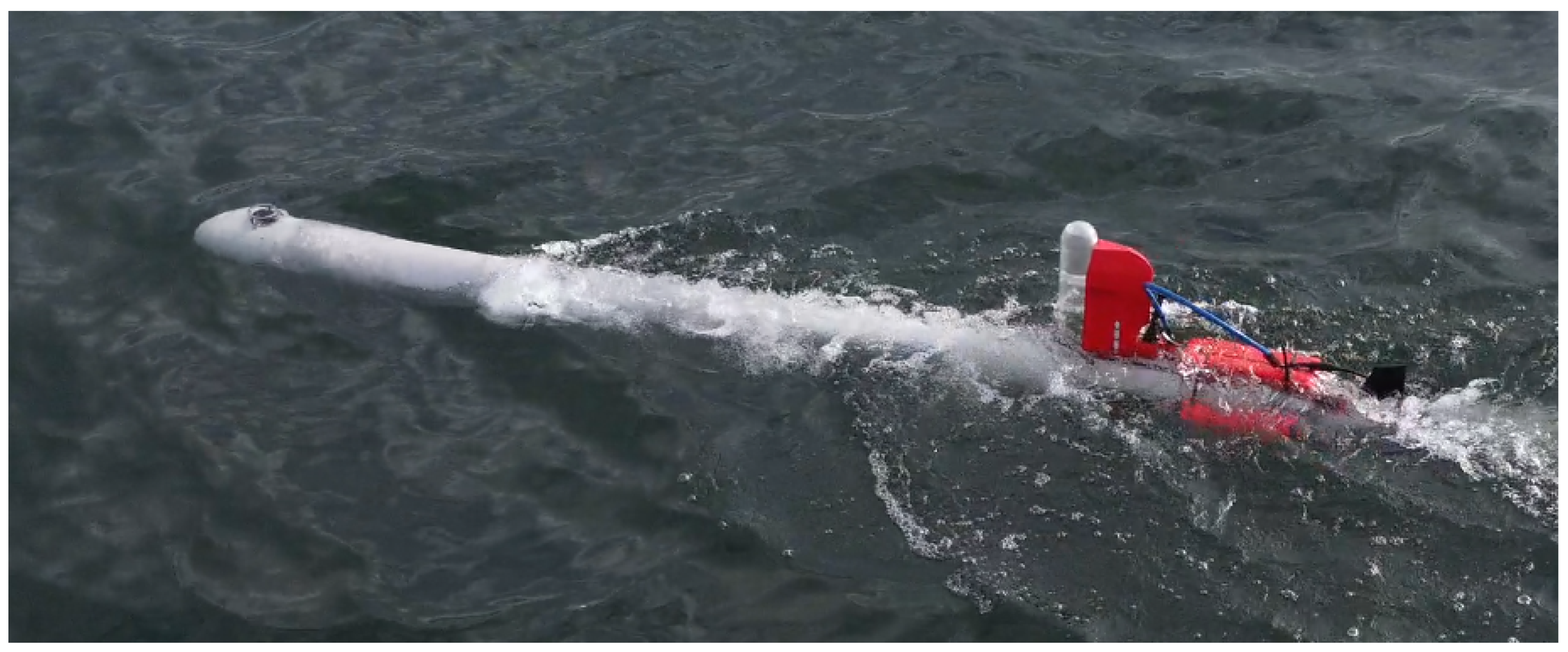
The scanning process is often conducted by a set of magnetometers (usually 2 or more) mounted on the wing pulled behind the ship or mounted on a formation of the AUVs scanning the interest area in parallel. An example of an AUV is a self-constructed vehicle shown in Figure 1.
In order to optimize the above process, one of the possibilities is to apply machine learning methods for the automatic identification of dangerous objects in particular UXO [2,3]. Considering that the scanned areas are usually calculated in square kilometers, automatization of data analysis should speed up the process. Even more, it is often possible to overcome the performance of human experts by more accurate classification of underwater objects by the use of machine learning models [4]. However, there is one potential weakness in the application of machine learning methods, which is the requirement for a large amount of good-quality training data. This issue is becoming even more important for the marine environment, where the collection of such data is associated with very high costs, labor-intensive and time-consuming. Additionally, the popular approaches for machine learning applications for UXO detection are based on electromagnetic induction (EMI) which is not applicable in underwater exploration, where the electromagnetic field is strongly attenuated. In that scenario, only magnetometers based on the magneto-static effect are useful, although they are much harder to correctly identify UXO from nonUXO objects [5].
In order to overcome the problem of lack of magnetometer-based data, we propose to build a full-feature digital twin of the UXO objects and their surroundings. Initially, a similar approach was already taken in [6] but the authors ignored remanent magnetization, which is in particular important within the water environment. Moreover, in [6] the authors have compared a commonly used dipole model of UXO objects which does not provide sufficiently good accuracy. Therefore, in our work, we propose a UXO model that is based on a digital twin modeled with remanent magnetization using the finite element method. This approach match more accurately simulates the shape of real ammunition are real signals. The quality of the model is calibrated using real measurements. Obtaining a validated model allows us to conduct a series of simulations to achieve full training datasets that contain simulations of a passage of a group of probes equipped with magnetometers over potential UXO-based scans. This approach faces several issues:
  • Achieving the agreement between the synthetic model (digital twin) and real-live data – that is the match between the data recorded by the real magnetometers and the data recorded in the virtual environment.
  • Obtaining the efficiency of the virtual environment, that is the need for very fast calculations of the digital twin, which result from the necessity of many recalculations of the digital model – different shapes of the identifying elements, different geographical orientation
  • Meshing problem considering the size of the 3D virtual environment that is a few meters large and the size of the UXO object that has walls a few millivoltmeters thick.
In this article we provide a detailed explanation of the process of developing such a digital twin and how we overcome the issues presented above. It must be noted that in the physical experiments conducted to validate the numerical model, we used a surrogate UXO object which was a pipe with a length of 343mm and 75mm of the diameter corresponding to the typical ammunition. The term typical ammunition is defined as ammunition considered dangerous while conducting work at the bottom of water reservoirs. The pipe was used for safety reasons and allowed us to carry out the experiments without the supervision of sappers. Similarly, in numerical experiments, the UXO object was modeled with a pipe, allowing to confirm and validate the model. When the numerical model is calibrated, the resultant dataset generated with the digital twin would enable us to verify whether it is possible to classify UXO / nonUXO objects based on the disturbance of the earth’s static magnetic field. Therefore, in the virtual environment, when generating the training set, we model not only the pipe under consideration, but also other pipes of different lengths and diameters that are too big or too small for UXO and other objects like ferromagnetic sheets, rings, etc.
The novelty of this article is:
  • Introducing digital twin for UXO classification for magnetic data including remanent magnetization
  • Empirical verification of the digital twin using data from physical experiments obtained using magnetometer sensor
  • Introducing a way for computational complexity reduction without sacrificing the results obtained from the digital twin
  • Identifying important properties of the digital twin which need to be implemented in order to achieve high comparability between physical data and numerical model
  • Introducing the way to create a dataset with multiple parallel virtual probes
The structure of this article is as follows: In Section 2 we provide the state-of-the-art in UXO identification and classification including digital twin models. Then in Section 3 we describe the mathematical model of the virtual environment, also introducing simplification of the model. In Section 4 an experiments comparing the digital twin and the physical model are discussed. The results of the experiments are provided in Section 5. The next section describes the details of how we created the training set. The last section concludes the manuscripts and summarizes the results obtained.

2. Related work

The subject of this article is a popular real-life problem that affects almost all countries. There are several topics that are important in terms of UXO classification. The first is the development of better sensors. For example, in [7] the authors indicate that the source of the noise in the transient electromagnetic sensors is mainly caused by the receiving coil where the noise is dominated by the internal thermal noise of the damping resistor. Reducing the bandwidth of the system and increasing the size of the coil effectively reduces internal noise. Another group of sensors constitutes magnetometers where two are very popular, the fluxgate magnetometers [8] which have the advantage of delivering a three-dimensional vector of the magnetic field, and optically pumped magnetometers (OPM) which gives more information at greater depth/height [9], although they return only the module of the signal. The OPMs are also under development and some recent developments include high-power off-resonant optical pumping; Mz configuration, where pumping light and magnetic field of interest are oriented parallel to each other; use of small alkali metal vapor cells of identical properties in integrated array structures. Another example of OPM optimization can be found in [10] where after sensor optimization the authors obtained a radio-optical cesium magnetometer sensitivity of 82.5 fT/ Hz , a resolution within 1 pT to an external magnetic field change, and a noise fluctuation of 0.2 pT for an integration time of 1 s. In addition to the sensors, an important stage is the recorded signal processing. There are several approaches to UXO identification. A nice overview can be found in a report [11] in which the authors provide general approaches. Among them, they identify two main approaches. The first method is based on fitting measured magnetic data neither TDEM, nor FDEM to a parametric model, and then using the recovered model parameters to classify the anomaly as UXO or non-UXO. Here, usually, a magnetic dipole model is used as a reference. The second approach is based on matching the measured data to the signature of known UXO and other objects. The authors also briefly discuss an approach based on SVM machine learning classification based on the parameters obtained after matching the signals to the model. The properties of the dipole model were extensively evaluated by many researchers. For example, in [6] the authors study the properties of the physical dipole, which are then compared favorably with alternative models, including the limited cases of prolate spheroids and other shapes. Additionally, in the work, the authors critically review the explicit modeling of the demagnetization properties of magnetic materials. A more advanced study on UXO numerical models was conducted in [12] where the authors compared the prolate spheroid model with two more realistic UXO geometries using a finite element method. The results obtained showed that the calculated dipole moment response for complex models that resemble actual UXO is up to 50% higher than the dipole moments for the prolate spheroid model. They also found that altering the shape of a model from a prolate spheroid to a complex shape has a greater effect on dipole moment than maintaining the same shape and altering the volume. Finally, they found that complex models more closely match actual field data than prolate spheroid models. An application of the recorded signals to the fitted model can be found in many works. For example in [13] the authors have used a Normalized Surface Magnetic Source (NSMS) model and a variant of the simple dipole model to the data recorded using electromagnetic induction (EMI). For discrimination, the authors used two sets of parameters: intrinsic parameters associated with the size, shape, and material composition of the target; and extrinsic parameters related to the orientation and location of the anomaly. They found that the discrimination performance significantly depends on the mathematical models: single dipole, multidipole, and NSMS. In particular, when the noise is low and the UXO is isolated, the basic methods work well, but with noise and multiple targets placed close to each other, the complete method is more attractive. Similar work can also be found in [14] and [15]. In the last, the authors tested the spheroid model of UXO objects and analyzed how the object behaves in terms of the height of the recorded magnetic field and the caliber of ammunition. The authors have also studied how shock demagnetization behaves. The problem of inverse can also be considered in terms of various approaches. For example, in [16] the authors considered two inversion approaches: cooperative or constrained inversion; and (2) joint inversion. Cooperative inversion is the process of using inversion parameters from one dataset to constrain the inversion of other data. In a true joint inversion, the target model parameters common to the forward models for each type of data are identified, and the procedure seeks to recover the model parameters from all the survey data simultaneously. Besides the inversion approaches, a key element is the direct inverse algorithm. For example, this topic was covered in [17] where the eigenvector decomposition of the magnetic gradient tensor was used to locate dipole-like magnetic sources, allowing automatic detection of dipole-like magnetic sources without estimating the magnetic moment direction. A similar approach has also been discussed in [18], where the authors proposed a new algorithm with a magnetic gradient tensor and singular value decomposition (SVD) to estimate the target position and characterization quickly and accurately. Another group of methods focuses on the use of electromagnetic data and the application of machine learning models [5]. In that article, the authors point out that "(...) magnetic data can only provide limited information about intrinsic target properties (i.e., size and shape) and are rarely used to classify detected targets as UXO and non-UXO." Therefore, most machine learning applications focus on EMI data. One of the early approaches to utilize machine learning methods, in particular the Probabilistic Neural Networks can be found in [19]. In [4] the authors discuss the concept of using linear genetic programming for UXO/nonUXO classification. A broader work that discusses many machine learning approaches can be found in [20] where the use of SVM and Probabilistic Neural Networks is discussed. Additionally, the authors discuss feature extraction techniques; in particular, they used a combination of a size and time-decay vector. As a result of their work, they developed the UXOLab software. The next example of utilizing a machine learning model is presented in [21] where the authors combine supervised learning such as SVM and neural networks with unsupervised learning such as Gaussian Mixture Modelling. As a feature space, they use features extracted from the EMI decay curves of the physics-based intrinsic, effective dipole moment, called the total Normalized Surface Magnetic Source (NSMS). They found that such a combination provides a reduction in the amount of required training data and allows for a convenient probabilistic interpretation of the classification.
A similar approach to ours can be found in [22] where the authors use total field magnetic responses obtained using the finite element method to train various classifiers. In particular, they used Random Forest, Support Vector Machine, and Neural Networks, additionally using several types of labels, where the based performance was obtained when the classes were derived from a multiclass self-organizing feature map (SOFM). Although in their work the authors assumed the lack of remanent magnetization which may be of particular importance in terms of the underwater classification. Another example of using machine learning methods in UXO classification was discussed in [3] where the authors used data obtained from ground penetrating radar. The results obtained allowed them to achieve an accuracy that ranged between 89% and 92%. Above, we noted several times the problem of remanent magnetization, where it is often assumed that, as a result of the hitting shock, a demagnetization occurs. But what is raised by many authors is that remanent magnetization can not be ignored and is very important. In particular, as indicated in [23] the remanent magnetization may remain. Moreover, the conducted experiments indicated that the opposite effect can occur, that the missile initially started with a very small remanence acquired a magnetic remanence in the direction of the inducing field at the time of impact, and the magnetic remanence is stable for time scales of up to one thousand years. Finally, it must be noted that in underwater research, many dangerous objects were sunk, therefore shock demagnetization cannot be assumed and needs to be included in the model.

3. The digital twin model

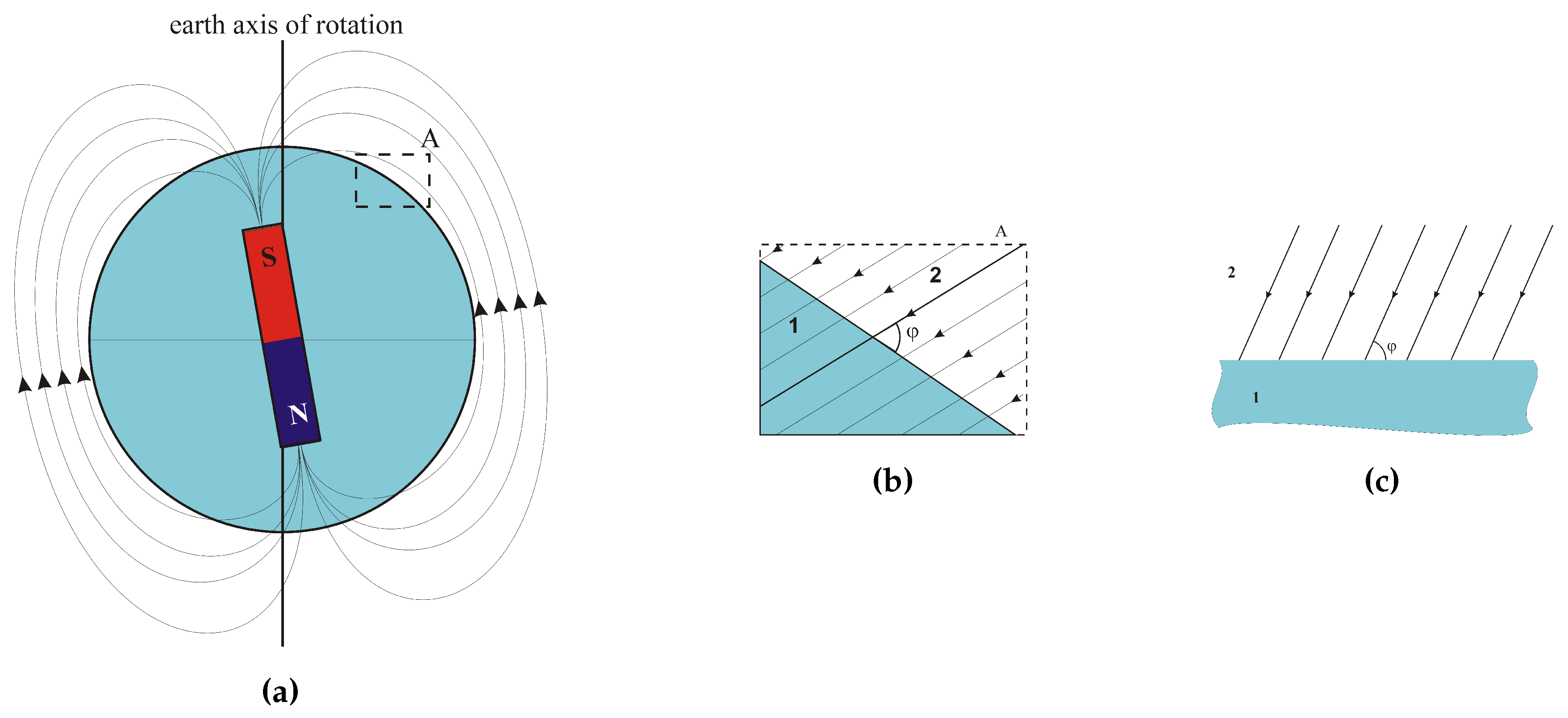
As mentioned in the introduction, one of the techniques used to detect dangerous objects is the study of the distortion of the earth’s magnetic field. This is a passive technique and requires the use of magnetic field sensors. As known, the earth is the source of the magnetostatic field, the distribution of the field on a global scale changes intensively (Figure 2), but on a local scale it can be assumed that the earth’s magnetic field is homogeneous, and the field lines are parallel to each other (Figure 2, Figure 2).
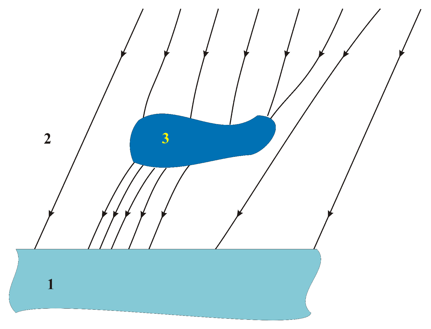
If the field force lines are not parallel, it means that there are objects (natural or anthropogenic) disturbing this distribution. To distort the distribution of the magnetic field (according to the formula 5), there must be a change in the magnetic permeability of the medium (change in magnetic permeability μ ) or an additional magnetic field must occur (magnetization M). It follows that the technique of studying changes in the earth’s magnetic field allows the detection of ferromagnetic objects. Theoretically, also diamagnetic or paramagnetic, but due to small differences in the value of relative magnetic permeability, the detection of paramagnetic and diamagnetic in the aspect analyzed in this article has no practical significance. An example of distortion of the magnetic field force lines by a ferromagnetic object is shown in Figure 3.
In order to create a digital twin of the UXO object two elements are needed these are a proper mathematical model of the system and an environment which will be used to apply this model.

3.1. Mathematical formulations

In terms of the mathematical model, it was assumed that within the virtual environment, is a homogeneous Earth’s magnetic field with an inclination of 67 o . Within this environment appears an isolated ferromagnetic object in particular a UXO object with known properties such as magnetic permeability. Initially, we assumed that no additional magnetization of the twin object, but during the experiments the object was extended with the magnetization vector. More formally, the equations allowing the analysis of the static magnetic field in the absence of current are derived from Maxwell’s equations. From Gauss’s law for a magnetic field in the form (1) and Ampere’s law in the form (2) [24].
· B = 0
× B = 0
where:
B - magnetic flux density.
Supplemented by the equation describing the magnetism in materials in the form (3) and the constitutive equation (4) [25]:
B = B 0 + μ 0 M
B = μ 0 μ r H
where:
B 0 - outside magnetic flux density,
μ 0 - the magnetic permeability of vacuum,
M - magnetization vector,
μ r - the relative magnetic permeability.
Finally, the equation describing the magnetostatic field without the presence of current for linear and isotropic media takes the form (5) [25] :
× 1 μ B M = 0
where:
μ - magnetic permaebility.

3.2. Modelling environment

The research presented in this article was based on a computational model prepared in the Gmsh - Getdp environment [26]. The Gmsh -Getdp software is a universal, open, still-developing numerical modeling environment that allows the creation of three-dimensional models of many physical fields. In this case, this program was used to model the static magnetic field.
During the preparation of the model, a typical numerical modeling problem was encountered, that is a large relative difference in the dimensions of objects in the computational model.
It was initially assumed that the model of the detected object has the approximate dimensions of a cylinder with a diameter of 20 mm to 300 mm and a length of 50 mm to 700 mm with a wall thickness of 5 mm to 15 mm [27,28]. On the other hand, the scanning/detection of the object occurs at a distance of 1 m to 4 m above it. Due to the typical, cone-shaped spread of the magnetic field disturbance, at a height of 1 m, a change in the magnetic field of 1 nT (the sensitivity of scalar cesium magnetometers is even pT) is detectable at a distance of approx. 8 m from the center of the projectile Figure 4, at a height of 4 m, this distance is 6 m. For such assumptions, the computational model must cover an area of 8 m x 8 m.
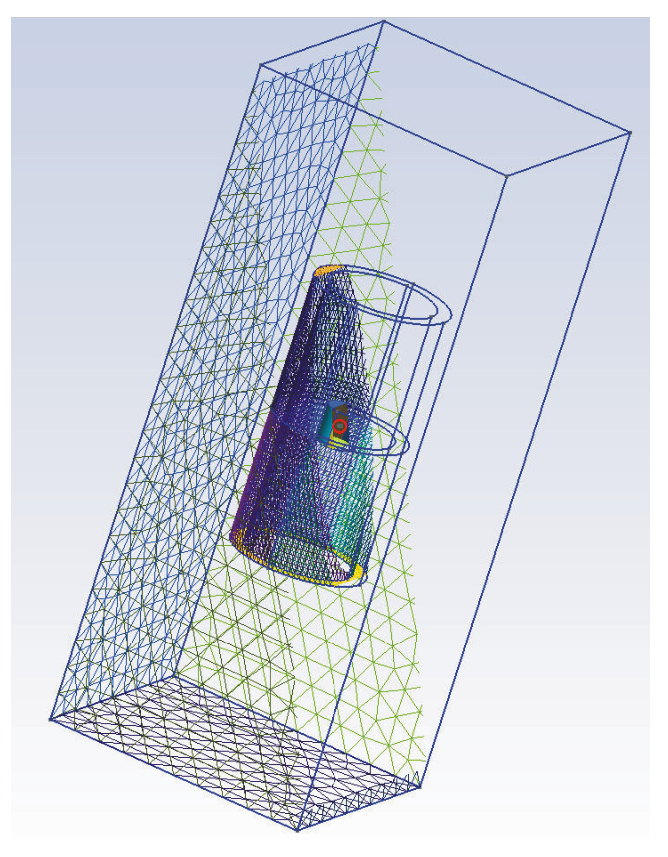
Such a large computing area in relation to the small wall dimensions of approx. 5 mm raises serious problems with correct model discretization. This manifested itself in two ways, either a very fine mesh, which guaranteed high accuracy of calculations at the expense of long calculation times, or in the other extreme case, a relatively coarse mesh (expanded in a classical way towards the outer borders of the calculation area), but then the calculation results at a great distance from the tested object were determined incorrectly. The compromise solution turned out to be an additional fineness of the mesh in the computational area of our interest Figure 5.
During the creation of meshes, we identified that proper results are obtained for mesh quality measures such as (SICN 1, Gamma 2, SIGE 3 [gmsh literature]) reaching values presented in Table 1. These values were used as a reference for all of the simulations.

3.3. Model simplification

As it was already indicated the model constituted a problem with proper meshing that resulted in a very high density of mesh nodes within the walls of the pipe. This resulted in a long computation time.
To solve this problem, it was decided to perform preliminary calculations for simplified models, replacing the thin-walled object (pipe) with a cylinder. Two simplified models were considered, one is a cylinder with relative magnetic permeability identical to the relative magnetic permeability of the exact model and the other simplified model, which is a cylinder of magnetic permeability equivalent to the magnetic permeability of the exact model. The equivalent permeability was determined based on the following equations (6) and (7). The μ r e - equivalent permittivity expresses volumetric equivalence.
μ r b V b = μ r e V r e
μ r e = μ r b V r b V r e
where:
μ r b - base relative permeability (permeability of original object),
μ r e - equivalent relative permeability,
V r b - volume of original object,
V r e - volume of the substitute object.
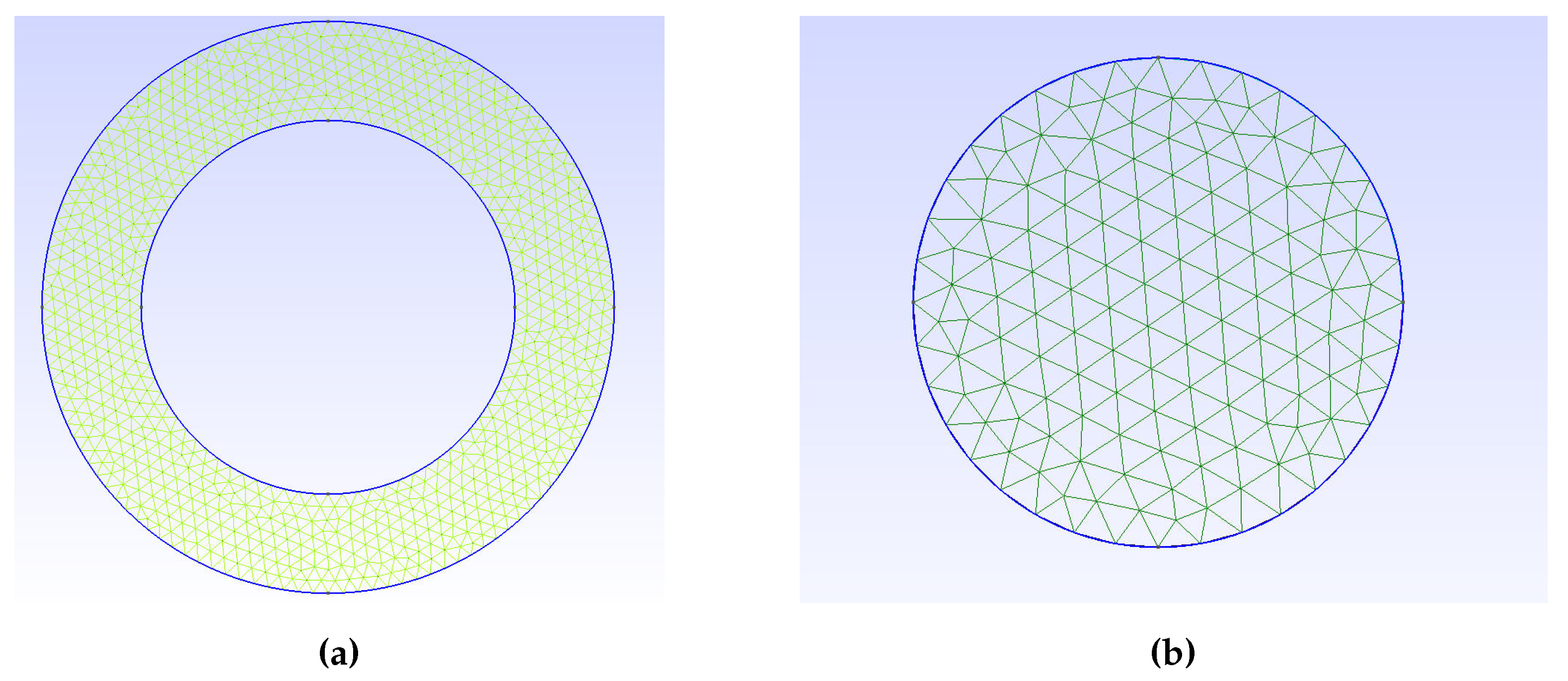
The use of a cylinder as a model made it possible to maintain the correctness of the discretization mesh in the object area and reduce the number of mesh nodes. Exemplary meshes for a pipe and a cylinder are shown in Figure 6 and Figure 6.
During the meshes creation, efforts were made to maintain similar measures of mesh quality for both models, mesh quality factors SICN, Gamma, SIGE only for objects are listed in Table 2, while mesh quality measures for the entire model along with the number of nodes are listed in the Table 3. Due to the model simplification, we were also able to reduce the computational complexity of the system. Less number of nodes results in less number of calculations. The benefit of a switch between a pipe and an equivalent cylinder is also shown in Table 3 in the last column.

4. Digital twin validation setup

The experiments consisted of 3 stages, which included: the construction of a mathematical-physical model, which has already been described in Section 3. Next, physical experiments were carried out involving the study of the UXO substitute with the use of magnetometers. The obtained results of the physical experiments were used to verify the quality of the mathematical model. In the next step, the mathematical model was optimized in order to reduce the computational complexity, without losing its performance. Below we present a description of each of these stages.

4.1. Empirical experiments

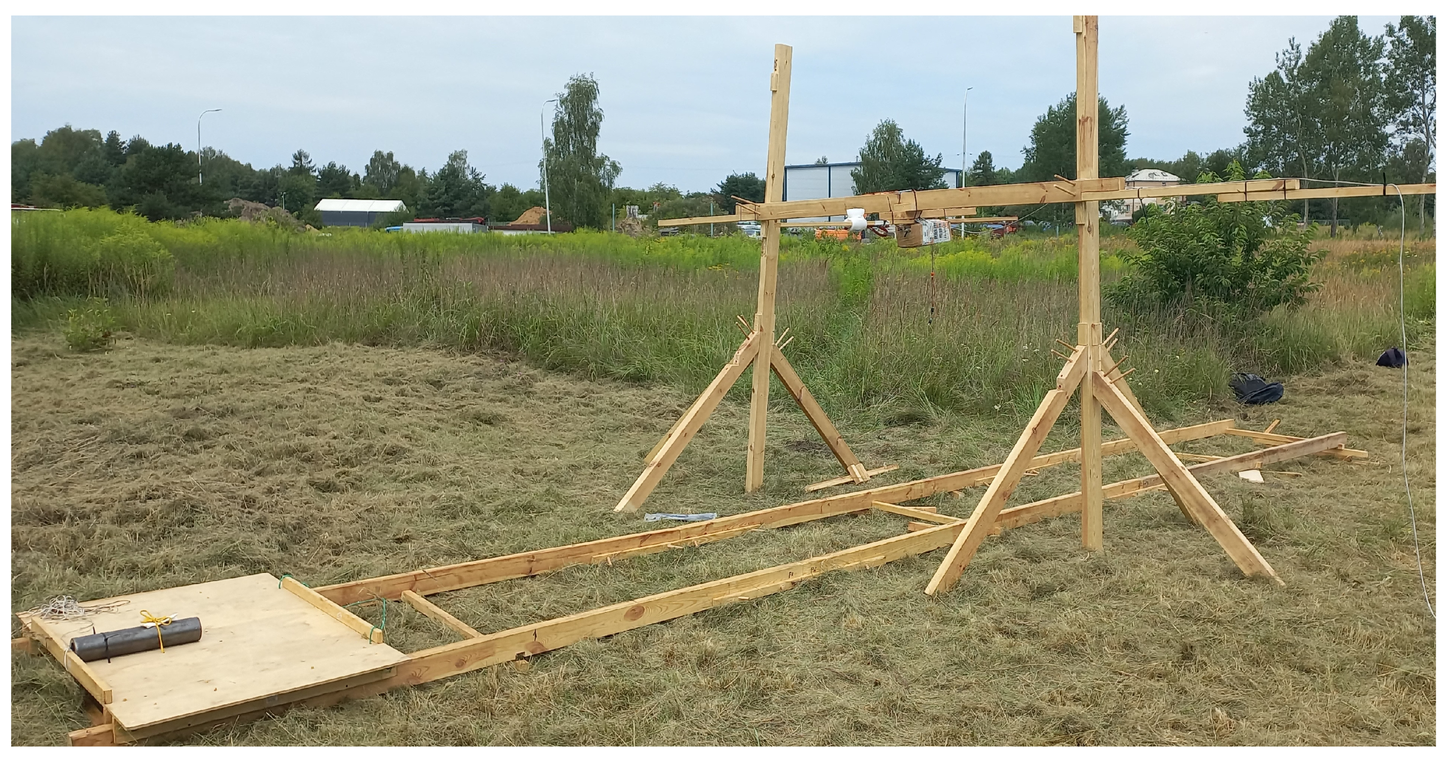
As already indicated the empirical experiments were conducted using a pipe Xmm long and 75mm in diameter. Because the water environment do not affect the magnetic field, we conducted the experiments out of the water, in an environment free of magnetic sources other than the natural Earth magnetic field. To assure a space free of ferromagnetic objects other than the UXO substitute the construction of the measuring station was made of wood without any nails or screws, every part was assembled with wooden nails. At the test stand, the magnetometer or magnetometers were mounted on a wooden frame above the test object - similar as it is during the mission with the use of AUV vehicles. The only difference was that in the tested environment it was the UXO object that moved. It was moved on the rails under the magnetometer, simulating a passage over the UXO object by the AUV containing the magnetometer. This allowed us to keep the computer station collecting the measurements out of the measuring station. The magnetometers were hanged on 1.4m above the rails, and the length of the rails was 7m. The magnetometer was located in the middle of the rails. A view of the measuring station is depicted in Figure 7.
In the experiments, we used the Geometrics MFAM LCS1005S magnetometer. The configuration of the measuring environment was as follows: orientation sensors for heading error cancellation, run mode: Low Noise and Two Independent Sensors, sampling frequency 1kHz, notch filter 50Hz.
For data collection, we used the LabView software package, and the obtained values were stored in CSV files. Next, the CSV files were loaded into self-developed environment, which was developed using Python and popular libraries such as Pandas, Numpy, SciPy.

4.2. Digital twin experiments

The digital twin of the virtual environment was built on the basis of the Gmsh [26] and GetDP [29] packages. The first tool was used to generate a mesh of the objects and a mesh of the environment. The results are then stored as a file which is delivered as input to the GetDP which is used for simulations. The simulation results, which are returned as a cloud of points coincided with the nodes of the mesh. Each node is described by a 3D vector with x,y,z components of the magnetic induction within the virtual environment.
In real applications, the magnetometers are often mounted on a wing pulled behind a ship, or a magnetometer is mounted on an AUV where an AUV formation (usually three or more) is conducting the measurements. In order to simulate such a magnetometer configuration we used the point cloud and an interpolator to achieve measurements with a fixed sampling rate. In the experiments, we used Matlab’s scatteredInterpolant function with natural, linear parameters, independently for each magnetic field component. Next, a path of probing was setup including the angle of sampling in relation to the N-S direction, the height of probing over the center of the ferromagnetic object, and the distance between particular magnetometers, assuming all sampling was conducted at the same height. Additionally, the model included the possibility of adding randomness to the probing. The randomness influences the distance between magnetometers, and height which results from imprecise positioning within the water environment. In the conducted experiments the randomness was set to 0. The obtained probing route was delivered to the input of the interpolator which returned sampled values of each magnetic field component.
It is important to note that the proposed approach is very efficient and for given object orientation allows conducting multiple experiments with many probing paths.

4.3. Data processing and signal comparison process

The data recorded from numerical and empirical experiments were further processed using Python in order to compare the obtained results. The general scheme of data processing is presented in Figure .
First, the data recorded during the physical experiments were filtered, because they were noisy. In order to reduce the effect of the noise the signal was sampled with a relatively high frequency (1kHz). This allowed using a moving average filter with a window size of 5 samples. That window size was enough to remove noise. Next, the signal was resampled with a frequency equivalent to the frequency used in the numerical experiments.
Next, the data obtained with the numerical simulations and physical experiments needed to be aligned to allow comparison. The problem of alignment resulted from differences in the length of the probing route (11m for the digital twin, and 7m for the physical experiments) and the location of the magnetometer within the physical experiment where it was not exactly in the middle of the route. The standard approach of signal alignment can be obtained using cross-correlation [30], but in the real scenario often multiple signals needed to be aligned simultaneously - one per magnetometer. In our experiments we used another measure, that is the mean square error between signals y and y ^ , where the value of n was under the subject of optimization.
n = a r g m i n j = 1 . . ( N M ) i = 1 M ( y j + i y ^ i ) 2
where:
  • N - the length of the signal recorded with a numerical model
  • M - the length of the signal recorded with the physical model
  • y = [ y 1 , y 2 , y M ] - the values of the signal recorded using physical model
  • y ^ = [ y ^ 1 , y ^ 2 , y ^ M ] - the values of the signal recorded using digital twin
  • n - the number of samples the signal y need to be moved forward or backward to align signal y ^
After finding n the signals were trimmed according to the shorter one. After the alignment of the signals, we calculated several performance measures. In the experiments, we used:
  • Root Mean Square Error (RMSE) - calculated as: R M S E ( y , y ^ ) = ( 1 N i = 1 N y i y ^ i 2 )
  • Mean Absolute Error (MAE) - calculated as: M A E ( y , y ^ ) = 1 N i = 1 N y i y ^ i
  • R 2 - calculated as: R 2 ( y , y ^ ) = 1 S S r e s S S t o t where S S r e s = i y i y ^ i 2 , and S S t o t = i y i y ¯ 2
These error measures were calculated assuming that the signal of the digital twin is denoted as y and the one from numerical experiments is denoted as y ^

5. Evaluation of the twin validation process

The first group of experiments was designed to achieve a full match between the digital twin and the physical experiments. First, we collected the data from the physical objects. For that purpose, the UXO object was scanned in different orientations and for different directions of scanning the object using AUV. In particular, we scanned in the following conditions:
  • UXO orientation - north-south, scanning route orientation north-south
  • UXO orientation - north-south, scanning route orientation east-west
  • UXO orientation - east-west, scanning route orientation east-west
  • UXO orientation - east-west, scanning route orientation north-south
  • UXO orientation - northeast-southwest, scanning route orientation east-west
  • UXO orientation - northeast-southwest, scanning route orientation north-south
  • UXO orientation - perpendicularly, scanning route orientation north-south
  • UXO orientation - perpendicularly, scanning route orientation east-west
For the performance calculation, the R 2 was used as the base reference performance metric because it combines the mean square error together with the level of noise. The obtained results for various performance metrics are shown in Table 4.
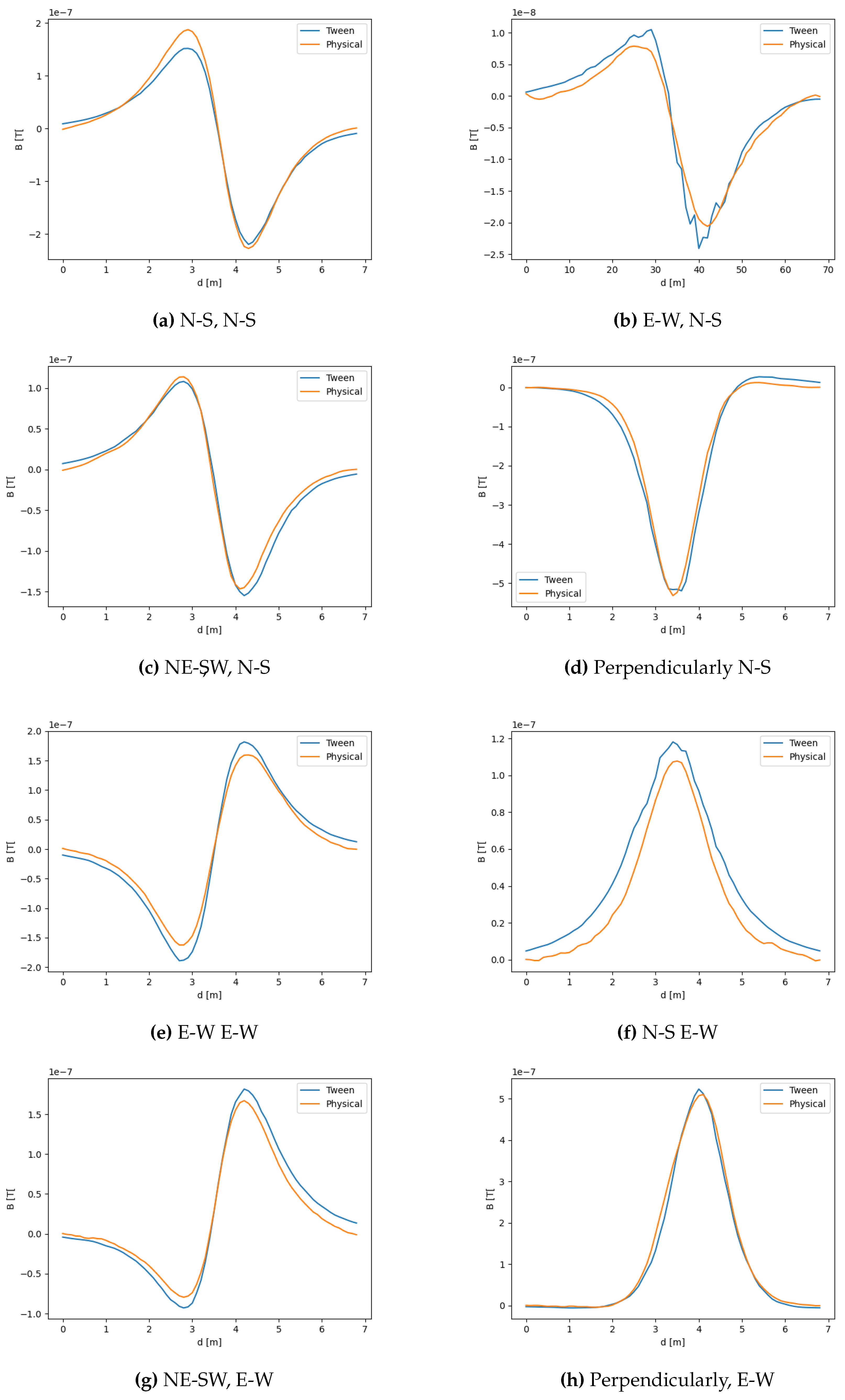
In the table, in almost all cases the obtained performances of R 2 are on the level of 0.99 or 0.95. For easier analysis of the results, the last column of the matrix indicates the amplitude of the signal, that is the difference between the maximum of the recorded physical signal and the minimum value of that signal. These results also indicate that the error rates nor RMSE or MAE are of order or two orders of magnitude smaller than the amplitude of the signal. The results indicate an almost perfect match. The quality of the match between the numerical model and the physical one is shown in Figure 8.
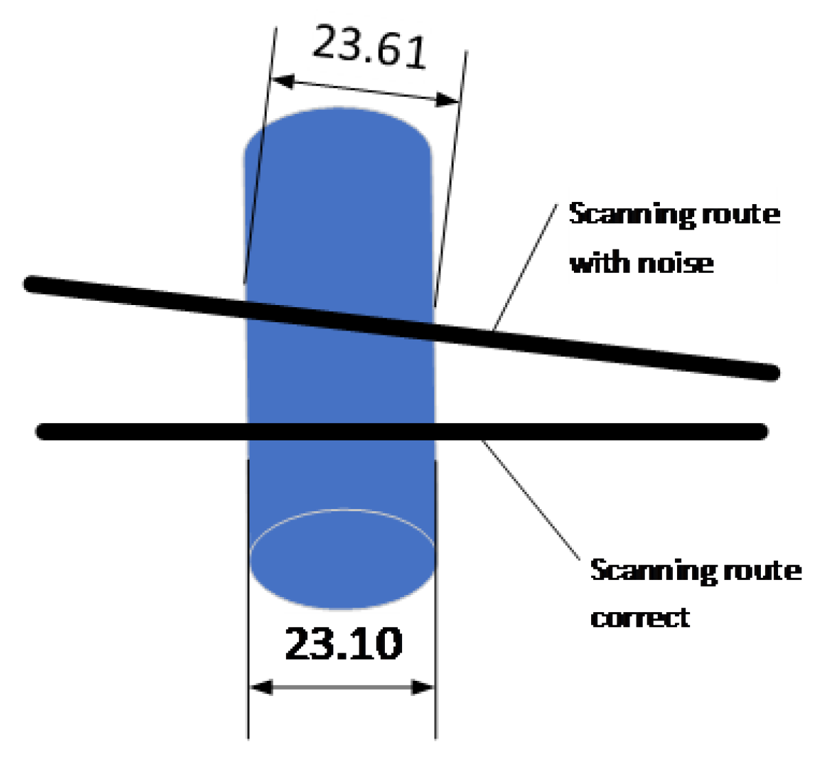
The only exception, that is R 2 = 0.8724 was obtained when UXO orientation was N-S and the scanning route was in E-W direction. This is also plotted in Figure 8f where it can be observed that the shape is almost right except for the magnitude of the signal. This can be explained by a small change in the orientation of the UXO object or E-W orientation that changes the active length of the object as shown in Figure 9.
Therefore, it can be concluded, that the digital twin very well matches the real physical signal.
The same calculations were also repeated for the cylinder substitute which allows for a significant reduction of the calculation time. In that case, we obtained similar results as presented in Table 5. Here, a small, insignificant increase in all error rates can be observed. Therefore, for the final training set creation, the cylinder substitute was used.

6. The training set creation procedure

The results presented above allowed us to conclude that the digital twin can be used for creating a training set for the machine learning purpose. Here, appeared some additional benefits of the tandem of GMesh and GetDP. These two tools are controlled by a script, therefore it was very easy to automatize the process of generalization of the digital twin to produce many objects of different orientations. In particular, the great advantage of this solution is full control based on scripts over all stages of building the digital twin. In a single step of data generation, the following parameters were introduced to the model in the Gmsh/GetDP environment:
  • strength and orientation (inclination) of the Earth’s magnetic field for the area for which experimental work was carried out (considered in the boundary conditions of the model),
  • dimensions and orientation of the UXO and potentially other objects,
  • material properties of this object (magnetic permeability, magnetization),
  • mesh density.
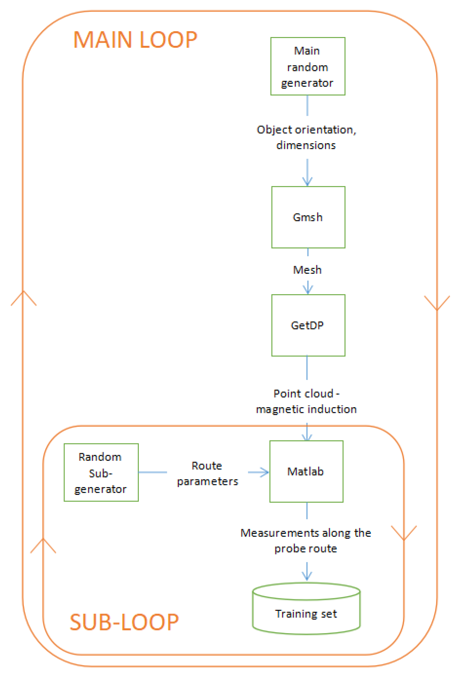
Figure 10 shows the scheme of generation of the training set. The process consists of two loops. In the main loop, a random generator provides orientations and sizes of modeled objects (in the range determined by the input parameters of the process). On this basis and the material parameters given at the input of the process, the Gmsh/GetDP model calculates the distribution of magnetic induction represented by a cloud of points. At this point, the inner subloop begins. The subgenerator randomizes the parameters of the probe route and, on this basis, the interpolator implemented in MATLAB simulates the magnetic field measurements during the passage of a group of probes. The scope of route randomization is also described by a set of input parameters of the generation process. After each flow simulation, another case is added to the training set.
For the final training set creation, most of the machine learning models need positive and negative cases (the so-called supervised learning). The final training set was obtained using a set of objects which are considered positive cases - UXO objects, and negative cases - non-UXO objects. The positive cases included substitute cylinders of predefined properties - the relation between the diameter and length of the cylinder, in particular, the length = 4 up to 6 diameters (that is the typical relationship between the length of the munition and its caliber). When the pipe has other properties it is considered a non-UXO object. In particular, as non-UXO objects, we considered munition that has too small caliber, less them 70mm, because it doesn’t cause significant danger for the works conducted on the bottom of the water reservoirs, and too large caliber> 200 mm and too long objects which were considered as simple long pipes - not a munition.
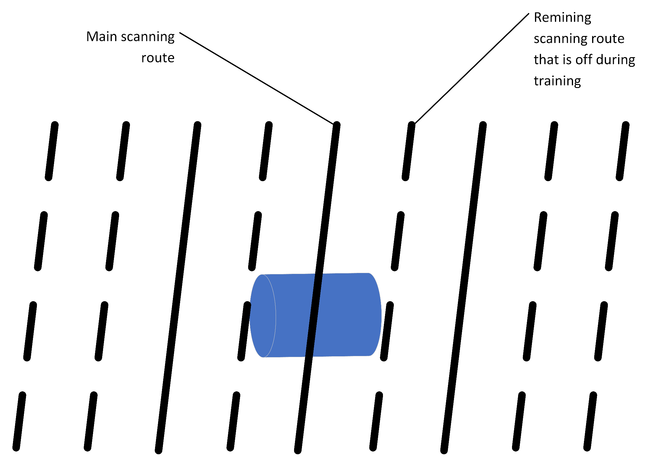
Additionally, as non-UXO objects also sheets of metal were considered. They had a thickness of 10mm to 30mm and different lengths and widths. The length and width were selected to have a similar mass to the UXO objects. The constructed model also allows the addition of two sources of magnetization of the objects. First, corresponds to the remanence magnetization resulting from the manufacturing or storage of the objects, and it can have any direction of the magnetization. The second source of magnetization depends on the time the object stayed at the bottom of the water reservoir. It results from the fact that many munitions were sunk right after the second world war, therefore they were magnetized by the Earth’s magnetic field. This allowed us to run around 1600 simulations of the digital twins of various objects and their parameters (some simulations failed due to meshing problems). Then for each digital twin, 30 random scanning routes were generated using the Matlab subroutine. In total, it resulted in around 48000 training samples. In the conducted simulations it was assumed that a single scanning route consisted of a formation of 9 virtual magnetometers parallel to each other as shown in Figure 11. These 9 parallel paths allow us to train and validate the prediction model in several scenarios. For example, by switching on and off particular routes we can simulate scenarios when a particular magnetometer is scanning on the side of the UXO object instead of the center, or to identify the effect of the distance between virtual magnetometers on the prediction quality.

7. Conclusions

In the manuscript, a process of creating a digital twin of the environment containing UXO and nonUXO objects was presented. The virtual environment was then optimized in terms of computational complexity and used to virtually scan the objects with virtual magnetometers. Such an environment has several advantages, it allows for easy collection of the training data for building machine learning models. It is safe, and do not require the supervision of the sapper, and allows for creating a massive training set in a range of several days. In our case, the calculations for creating the training set consisting of 46,000 samples took 3 days on a single two-processor machine (2xAMD EPIC processor and 512GB RAM), whereas collecting the data for the physical experiments to collect 8 scans took a single day.
In the manuscript, we have also shown how to simplify the model to speed up the calculations without sacrificing the quality of the obtained results. The proposed solution significantly reduces the number of nodes of the mash which resulted in reducing the calculation time by 1/3. In general, we have shown that the approach of building virtual environments for generating data for training machine learning models is not only possible for vision problems but can be also applied to other environments, although it requires careful tuning of the model to achieve results comparable to the one recorded with physical sensors. An example of such an environment is detecting the UXO objects in an underwater environment using magnetometer sensors. In the manuscript, we omit the problem of creating a machine learning model as it is the subject of another article and is out of the scope of this article.

Author Contributions

Conceptualization, M.B. and S.G.; methodology, M.B., and S.G. and R.P.; software, R.P.and M.B. and P.S and S.G.; validation, R.P. and P.S. and M.B.; formal analysis, S.G. and T.W.; investigation, R.P.and M.B. and P.S and S.G.; resources, M.B. and P.S.; data curation, R.P. ; writing—original draft preparation,R.P.and M.B. and P.S and S.G.; writing—review and editing,T.W.; visualization, R.P. an P.S.; supervision, M.B. and T.W.; funding acquisition, M.B. and P.S. All authors have read and agreed to the published version of the manuscript.

Funding

This research was partially funded by the Silesian University of Technology proj. no BK-221/RM4/2023; 11/040/BK_23/0029 and by Polish National Centre for Research and Development (NCBR) under project number POIR.01.01.01-00-1088/20.

Conflicts of Interest

The authors declare no conflict of interest.

References

  1. Przeciwdziałanie zagrożeniom wynikającym z zalegania materiałów niebezpiecznych na dnie Morza Bałtyckiego. Technical Report 192/2019/P/19/068/LGD, Najwyższa Izba Kontroli, 02-056 Warszawa, ul. Filarowa 57, 2020.
  2. Heagy, L.J.; Oldenburg, D.W.; Pérez, F.; Beran, L. Machine learning for the classification of unexploded ordnance (UXO) from electromagnetic data. In Proceedings of the SEG International Exposition and Annual Meeting. OnePetro; 2020. [Google Scholar]
  3. Núñez-Nieto, X.; Solla, M.; Gómez-Pérez, P.; Lorenzo, H. GPR signal characterization for automated landmine and UXO detection based on machine learning techniques. Remote sensing 2014, 6, 9729–9748. [Google Scholar] [CrossRef]
  4. Deschaine, L.M.; Hoover, R.A.; Skibinski, J.N.; Patel, J.J.; Francone, F.; Nordin, P.; Ades, M. Using Machine Learning to Complement and Extend the Accuracy of UXO Discrimination Beyond the Best Reported Results of the Jefferson Proving Ground Technology Demonstration. SIMULATION SERIES 2002, 34, 46–52. [Google Scholar]
  5. Beran, L.; Zelt, B.; Billings, S. Detecting and classifying UXO. J. ERW Mine Action 2013, 17, 57–63. [Google Scholar]
  6. Furey, J.S.; Butler, D.K. The physical dipole model and polarizability for magnetostatic object parameter estimation. Journal of Environmental & Engineering Geophysics 2011, 16, 49–60. [Google Scholar]
  7. Wang, H.; Chen, S.; Zhang, S.; Yuan, Z.; Zhang, H.; Fang, D.; Zhu, J. A high-performance portable transient electro-magnetic sensor for unexploded ordnance detection. Sensors 2017, 17, 2651. [Google Scholar] [CrossRef] [PubMed]
  8. Gavazzi, B.; Le Maire, P.; de Lépinay, J.M.; Calou, P.; Munschy, M. Fluxgate three-component magnetometers for cost-effective ground, UAV and airborne magnetic surveys for industrial and academic geoscience applications and comparison with current industrial standards through case studies. Geomechanics for Energy and the Environment 2019, 20, 100117. [Google Scholar] [CrossRef]
  9. Fassbinder, J.W. Magnetometry for archaeology. Encyclopedia of geoarchaeology, 2017; pp. 499–514. [Google Scholar]
  10. Ding, Z.; Yuan, J.; Long, X. Design and optimization of a high-sensitivity radio-optical cesium magnetometer. Optics & Laser Technology 2019, 119, 105573. [Google Scholar]
  11. Goodson, R.A.; Morgan, J.C.; Butler, D.K.; Fields, M.P.; Bennett Jr, H.H.J.; Demoss, T. Unexploded Ordnance (UXO) Data Analysis System (DAS) 2009.
  12. Churchill, K.M.; Link, C.; Youmans, C.C. A comparison of the finite-element method and analytical method for modeling unexploded ordnance using magnetometry. IEEE transactions on geoscience and remote sensing 2011, 50, 2720–2732. [Google Scholar] [CrossRef]
  13. Shubitidze, F.; Fernández, J.; Barrowes, B.; O’Neill, K.; Shamatava, I.; Bijamov, A. Comparison of the physically complete model with a simple dipole model for UXO detection and discrimination. In Proceedings of the Detection and Sensing of Mines, Explosive Objects, and Obscured Targets Xv. SPIE, 2010, Vol. 7664; pp. 81–92.
  14. Pasion, L.R.; Billings, S.D. Dipole Models for UXO Discrimination at Live Sites. Technical report, Black Tusk Geophysics Vancouver Canada, 2017.
  15. Butler, D.K.; Simms, J.E.; Furey, J.S.; Bennett, H.H. Review of magnetic modeling for UXO and applications to small items and close distances. Journal of Environmental and Engineering Geophysics 2012, 17, 53–73. [Google Scholar] [CrossRef]
  16. Butler, D.K.; Pasion, L.; Billings, S.D.; Oldenburg, D.; Yule, D.E. Enhanced discrimination capability for UXO geophysical surveys. In Proceedings of the Detection and Remediation Technologies for Mines and Minelike Targets VIII. SPIE, 2003, Vol. 5089; pp. 958–969.
  17. Zuo, B.; Wang, L.; Chen, W. Full tensor eigenvector analysis on air-borne magnetic gradiometer data for the detection of dipole-like magnetic sources. Sensors 2017, 17, 1976. [Google Scholar] [CrossRef] [PubMed]
  18. Wang, L.; Zhang, S.; Chen, S.; Luo, C. Fast Localization and Characterization of Underground Targets with a Towed Transient Electromagnetic Array System. Sensors 2022, 22, 1648. [Google Scholar] [CrossRef] [PubMed]
  19. Hart, S.J.; Shaffer, R.E.; Rose-Pehrsson, S.L.; McDonald, J.R. Using physics-based modeler outputs to train probabilistic neural networks for unexploded ordnance (UXO) classification in magnetometry surveys. IEEE Transactions on Geoscience and Remote Sensing 2001, 39, 797–804. [Google Scholar] [CrossRef]
  20. Billings, S. Data Modeling, Feature Extraction, and Classification of Magnetic and EMI Data, ESTCP Discrimination Study, Camp Sibert, AL. Demonstration Report. Technical report, SKY RESEARCH ASHLAND OR, 2008.
  21. Bijamov, A.; Shubitidze, F.; Fernandez, J.P.; Shamatava, I.; Barrowes, B.E.; O’Neill, K. Comparison of supervised and unsupervised machine learning techniques for UXO classification using EMI data. In Proceedings of the Detection and Sensing of Mines, Explosive Objects, and Obscured Targets XVI. SPIE, 2011, Vol. 8017; pp. 56–66.
  22. Bray, M.P.; Link, C.A. Learning machine identification of ferromagnetic UXO using magnetometry. IEEE Journal of Selected Topics in Applied Earth Observations and Remote Sensing 2014, 8, 835–844. [Google Scholar] [CrossRef]
  23. Schultze, V.; Schillig, B.; IJsselsteijn, R.; Scholtes, T.; Woetzel, S.; Stolz, R. An optically pumped magnetometer working in the light-shift dispersed M z mode. Sensors 2017, 17, 561. [Google Scholar] [CrossRef] [PubMed]
  24. Nunes, A.S.; Dular, P.; Chadebec, O.; Kuo-Peng, P. Subproblems Applied to a 3-D Magnetostatic Facet FEM Formulation. IEEE Transactions on Magnetics 2018, 54, 1–9. [Google Scholar] [CrossRef]
  25. Magnetostatics, Theory. https://www.comsol.com/multiphysics/magnetostatics-theory, 2019.
  26. Geuzaine, C.; Remacle, J.F. Gmsh: A 3-D finite element mesh generator with built-in pre-and post-processing facilities. International journal for numerical methods in engineering. 2009, 11, 1309–1331. [Google Scholar] [CrossRef]
  27. of Suppl Publication Chief Inspector of Armaments, A.M. Ammunition bulletine no 51. https://stephentaylorhistorian.files.wordpress.com/2020/02/ammunition-bulletin-no-51.pdf, 1946.
  28. Gov, U. German explosive ordnance vol. 2. https://stephentaylorhistorian.files.wordpress.com/2020/09/op-1666-german-explosive-ordnance-volume-2.pdf, 1946.
  29. Geuzaine, C. GetDP: A general finite-element solver for the de Rham complex. In PAMM: Proceedings in Applied Mathematics and Mechanics 2007, 7, 1010603–1010604. [Google Scholar] [CrossRef]
  30. Bourke, P. Cross correlation. Cross Correlation”, Auto Correlation—2D Pattern Identification 1996.
1
SICN -signed inverse condition number
2
Gamma - inscribed radius / circumscribed radius
3
SIGE - signed inverse error on the gradient of FE solution
Figure 1. Autonomous underwater vehicle developed for UXO detection.
Preprints 75531 g001
Figure 2. Earth magnetic field a) global view, b) local view of A detail c) local view of A detail in classical perspective (earth surface horizontal); 1 - earth; 2 - air (or water); φ - magnetic field inclination
Preprints 75531 g002
Figure 3. Distorted Earth magnetic field 1 - earth; 2 - the surroundings of the object (air, water); 3 - magnetic object;
Preprints 75531 g003
Figure 4. Exemplary relative ( Δ B ) change of the magnetic field at the height of: a) 1 m; b) 2 m; c) 3 m; d) 4 m over the ferromagnetic object - plot from simulation, external dimension of the plot area is 6 m x 6 m.
Preprints 75531 g004
Figure 5. General view of the discretization mesh, the object in the center of the calculation area in red circle (almost invisible).
Preprints 75531 g005
Figure 6. Discretization meshes a) for a pipe (original object); b) for a cylinder (substitute object)
Preprints 75531 g006
Figure 7. The magnetometer measuring station.
Preprints 75531 g007
Figure 8. Visual representation of the match between the digital twin and the real magnetometer data.
Preprints 75531 g008
Figure 9. The source of the disagreement between the measurements and the model.
Preprints 75531 g009
Figure 10. Scheme of the training set generation process.
Preprints 75531 g010
Figure 11. The parallel scanning routes. When building the model it can be assumed that only 3 routes were available with different relation to the center of the object. Solid lines represent such a case, while a dashed line represents routes that were off during preprocessing of the final training set for the model.
Preprints 75531 g011
Table 1. Measures of mesh quality for the tested object.
SICN Gamma SIGE
0.5164 0.4928 0.7164
Table 2. Measures of mesh quality for the tested object.
Model SICN Gamma SIGE
pipe 0.5164 0.4928 0.7164
cylinder 0.5784 0.5504 0.7383
Table 3. Measures of mesh quality, number of nodes and calculation time for the entire model.
Model SICN Gamma SIGE Nodes number Calculation time
pipe 0.6439 0.6085 0.7444 155215 00:32:56.6805432
cylinder 0.6945 0.6486 0.7517 78601 00:13:15.7674002
Table 4. Resoults comparing the physical system with the digital twin.
UXO orientation Scanning orientation R 2 RMSE MAE MAX-MIN
N-S N-S 0.9849 1.37E-08 1.04E-08 4.15E-07
E-W N-S 0.9507 1.79E-09 1.49E-09 2.85E-08
NE-SW N-S 0.9850 8.50E-09 7.14E-09 2.61E-07
Perpendicularly N-S 0.984168 2.08E-08 1.64E-08 5.44E-07
E-W E-W 0.9687 1.57E-08 1.46E-08 3.22E-07
N-S E-W 0.8724 1.24E-08 1.15E-08 1.08E-07
NE-SW E-W 0.9680 1.22E-08 1.09E-08 2.46E-07
Perpendicularly E-W 0.9933 1.38E-08 8.90E-09 5.14E-07
Table 5. Comparison of error rates between the pipe and a cylinder substitute.
UXO orientation Scanning orientation R 2 RMSE MAE MAX-MIN
Pipe N-S N-S 0.9849 1.37E-08 1.04E-08 4.15E-07
Cylinder N-S N-S 0.9843 1.40E-08 1.07E-08 4.15E-07
Disclaimer/Publisher’s Note: The statements, opinions and data contained in all publications are solely those of the individual author(s) and contributor(s) and not of MDPI and/or the editor(s). MDPI and/or the editor(s) disclaim responsibility for any injury to people or property resulting from any ideas, methods, instructions or products referred to in the content.
Copyright: This open access article is published under a Creative Commons CC BY 4.0 license, which permit the free download, distribution, and reuse, provided that the author and preprint are cited in any reuse.
Prerpints.org logo

Preprints.org is a free preprint server supported by MDPI in Basel, Switzerland.

Subscribe

© 2024 MDPI (Basel, Switzerland) unless otherwise stated