1. Introduction
Object tracking is constantly determining a moving object's trajectory from measurements taken by one or more sensors [
1]. Single-object tracking (SOT) [
2] and Multi-object tracking (MOT) [
3,
4,
5,
6,
7] are two main categories of object tracking methods (MOT). When using SOT, the tracker follows a single, predetermined object. Object tracking is required as soon as a target appears in the first frame and must be tracked in all subsequent frames. Multi Object Tracking (MOT) necessitates a detection step to identify all targets of a particular class and monitor them individually without any previous information of their appearance or amount. This is a far more difficult endeavor, as a number of issues, such as object occlusion and objects with similar looks, may make tracking more difficult [
1]. In object tracking, track loss occurs when false measurements are used in a tracking filter, which causes the estimation error to diverge [
8].
Recently, the state-of-the-art MOT research has centered on two methods: (i) tracking by detection [
9,
10,
11,
12,
13,
14] and (ii) joint tracking and detection [
15,
16]. In this work, our focus is detection by tracking. During tracking by detection, an object detector is used to detect objects in a frame and provide that detection information to the object tracking algorithm to perform the frame-to-frame association of the objects. For instance, if five objects were detected in a given frame, five distinct bounding boxes would be generated and tracked throughout all future frames. However, detecting and tracking frame-by-frame is laborious and may prevent MOT from being executed in real-time, thus reducing the level of object-tracking performance. Other challenges facing object tracking include the lack of balance between tracking speed and accuracy, background distractions, noise (such as fog) in the background, multi-spatial scaled objects, and occlusion.
As previously mentioned, the initial step of tracking by detection algorithm is to detect the objects that need to be tracked. Autonomous vehicles (AVs) often use a variety of sensors, including cameras, lidars, and radars, to detect objects such as (pedestrians, cars, trucks, bicyclists, traffic lights/signs, etc.) in their path [
17,
18,
19]. However, inclement weather, including heavy fog, snow, rain, and sandstorm, can drastically reduce sensor performance [
20,
21,
22,
23,
24,
25]. For instance, low visibility in heavy foggy weather makes it difficult for cameras to detect objects, increasing the likelihood of collisions and fatalities [
24,
26]. On the other hand, there is a loss of reflectivity and an inaccuracy in distance measurement when using lidar in fog. By monitoring how much energy is reflected from radio waves, radars can calculate the range and speed of an object using the doppler effect. Thus, radars outperform cameras and lidars in bad weather and remain consistent regardless of atmospheric conditions. The data from radars is too sparse for object classification due to the low density of radar point clouds [
27,
28]. However, AVs' radar and camera fusion systems can provide complementary information for detected objects [
19,
28,
29,
30].
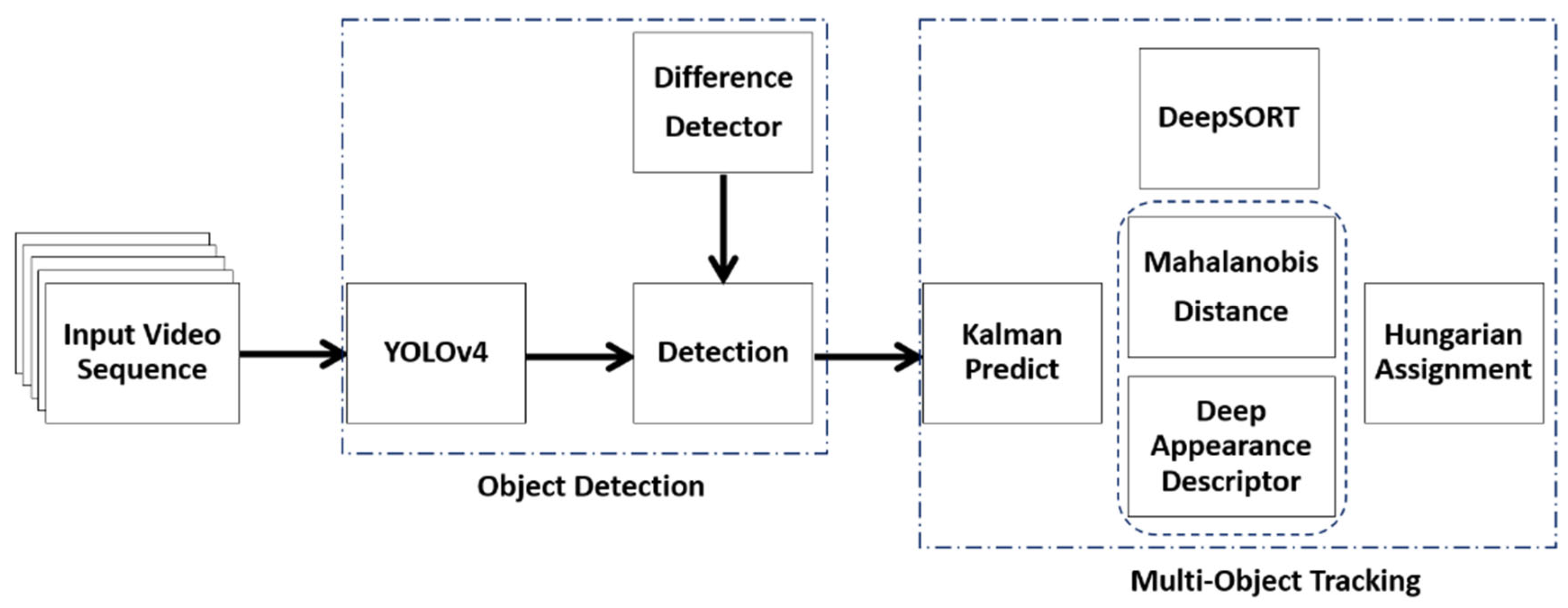
Wojke et al. proposed DeepSORT [
10] that uses YOLOv4 for the detection phase. The traditional YOLOv4 model is a single sensor system that takes only video sequence as input. The original DeepSORT a simple neural network for deep appearance descriptor such that the feature map extracted is prone to losing relevant details about the track being matched with a given detection in fog. In heavy fog, targets with a high degree of appearance similarity on the detection frame are more likely to be mismatched with the wrong predictions resulting in identity switches or track failures. Matching inaccuracies occur when objects of various sizes are on the same detection frame. Tracking small, colored, distant, and widely varied sizes objects can be challenging and yield inaccurate outcomes if the background is too noisy or excessively busy with objects of similar color. It is simpler for object detectors to identify and track objects with a uniform background. Therefore, an input frame containing objects with strong color contrast works best for object tracking. It is important to have a solid framework that can boost detection and tracking capabilities while decreasing the number of identity switches and track failures in fog. In this paper, based on the DeepSORT algorithm [
10] in
Figure 1, we present an improved deep learning-based multi-object tracking approach in
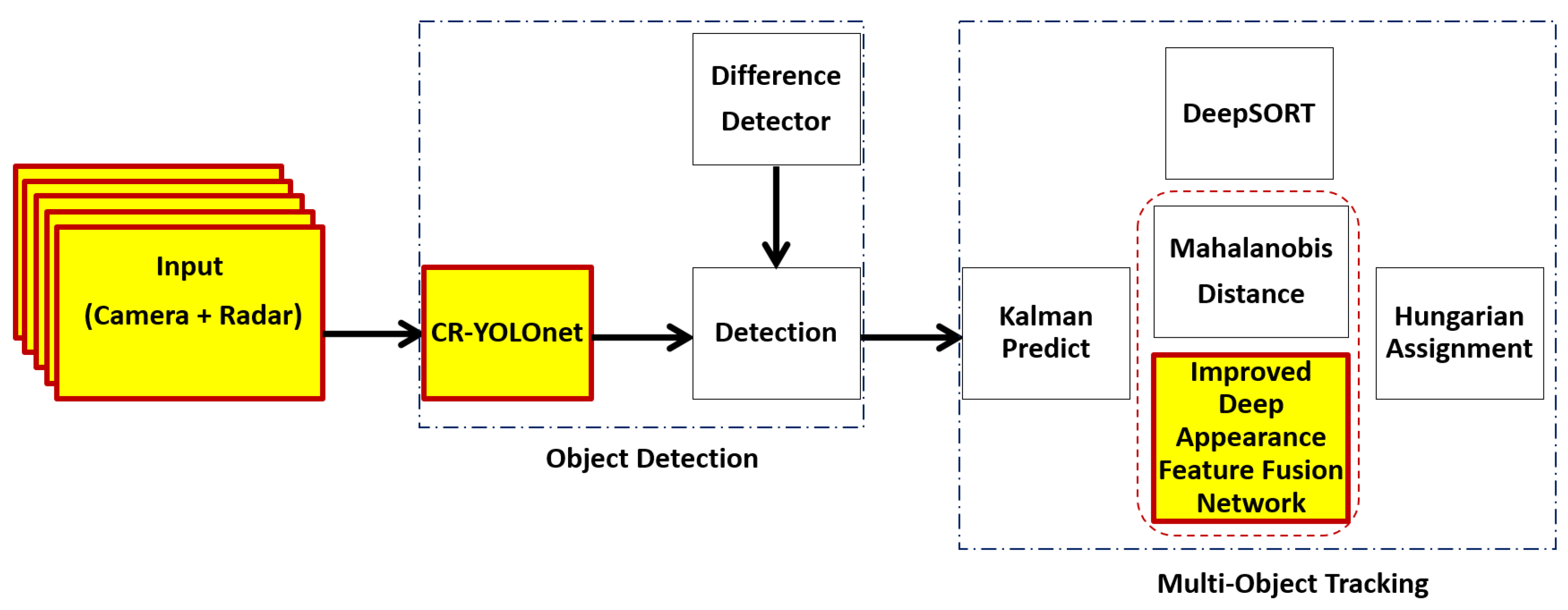
Figure 2. We address: (i) the issues of background distractions and noise caused by fog that can cause detection and prediction mismatch and (ii) the balance between tracking accuracy and tracking speed.
We make the following contributions to achieve improved tracking speed and tracking accuracy under foggy weather conditions:
Instead of a single sensor modal system (video sequence only) used for the detection phase in [
9,
10], we employed our deep camera-radar fusion network (CR-YOLOnet model) [
31] for faster and more accurate object detection in the detection phase of our improved deep learning-based MOT in
Figure 2. Our CR-YOLOnet model reached an accuracy (mAP at 0.50) of 0.849 and a speed of 69 fps for small and distant object detection under medium and heavy fog conditions.
We simulated a real-time autonomous driving environment in CARLA [
32] simulator. In addition to the radar and camera sensors, we obtain semantic labels of the ego vehicle environment using semantic segmentation cameras. The semantic segmentation camera presents each object in its field of vision with a distinct color corresponding to the predetermined object category (label). We fed the semantic labels into the segmentation module of our own deep convolutional neural network-based appearance descriptor.
We replaced the basic convolutional neural network used for appearance descriptor in DeepSORT with our deep convolutional neural network. Our deep appearance descriptor uses cross-stage partial connection (CSP)-based backbone for low-level feature extraction and feature pyramid network (FPN)-based neck for multi-scale level feature vectors to address objects of different sizes. We incorporate GhostNet into our deep appearance descriptor to replace the traditional convolutional layers used in standard neural networks. Using GhostNet helps to: (i) generate more features, thus, improving the integrity of the feature extracted for an accurate detection and prediction match, (ii) reduce the number of parameters, computational complexities, and cost, thus, improving tracking speed without diminishing the output feature map.
We incorporate a segmentation module to add rich semantic information to the low-level appearance feature map generated using semantic labels. With semantic labels, the segmentation module can help the deep appearance descriptor distinguish between objects with close appearances and similarities even when the background is noisy.
Our proposed method performed better than YOLOv5 + DeepSORT. Especially under heavy fog conditions, our results show that the multi-object tracking accuracy (MOTA) increased by 35.15%, the multi-object tracking precision (MOTP) increased by 32.65%, the speed increased by 37.65%, and identity switches (IDS) reduced by 46.81%. The remaining parts of this paper are structured as follows: we discuss the related studies in section 2, we describe our materials and methodology in section 3, in section 4 is where we present our improved appearance feature extraction network, we present our results and discussion in chapter 5, and section 6 consist of the conclusions.
2. Related Works
2.1. Object Detection
In literature, many deep learning models [
33,
34,
35,
36] have provided excellent detection accuracy and speed for object detection tasks under favorable weather circumstances. AlexNet, suggested by Krizhvsky et al. [
37], was the first convolutional network used for image feature extraction, ushering in the current era of deep feature extraction. In our previous work [
31], we did a comprehensive review of camera-only along with camera and radar fusion-based object detection methods. Some of the camera-only approaches include SSD proposed by Liu et al [
38], YOLO proposed by Redmon et al. [
39], and its derivatives [
40,
41,
42,
43,
44], RCNN proposed by Girshick et al. [
45], and its derivatives [
46,
47,
48]. Some camera-radar approaches include [
28,
49,
50,
51,
52]. Although these methods provide excellent detection accuracy and speed in favorable weather, they are extremely inefficient when used in foggy weather [
25]. There is a limited camera-radar approach in the literature for object detection under foggy weather conditions. Because of the tradeoff between detection speed and accuracy, existing methods have a very limited range of use in foggy weather conditions. Recently, we proposed a deep learning-based radar and camera fusion (CR-YOLOnet) [
31]based on YOLOv5[
44] for object detection in foggy weather conditions. In [
31], we gave a comprehensive overview of YOLOv5. When detecting small and distant objects, our small CR-YOLOnet model achieved a balance between accuracy and speed and performed better than YOLOv5. The small CR-YOLOnet model reached an accuracy (mAP at 0.50) of 0.849 and a speed of 69 fps for medium and heavy fog conditions.
2.2. Tracking by Detection
Tracking by detection methods uses existing information about where objects are located along with the predicted information to produce a time-variant association model for object tracking. The multiple hypothesis tracking (MHT) approach is one of the first MOT techniques proposed in the literature [
53,
54,
55]. Delaying complex data association determinations until more data is collected is crucial to the MHT approach. Many methods [
9,
10,
56] have used the Kalman filter (KF), which considers both the current detections (bounding boxes) as input measurements and prior predictions to estimate where the target objects would appear in the next frame. Previous research has used the KF method as a velocity and motion model to enhance object associations. Particle filter algorithms were also studied for effective initialization and learning phase multi-object tracking [
57]. However, tracking multi-scale targets and identity switches (IDS) continues to be challenging. Because of advances in computing power and the concept of deep learning, better tracking by detection methods (such as simple online and real-time tracking (SORT) [
9], DeepSORT [
10], etc.) have been developed.
Bewley et al. [
9] suggested the SORT algorithm that employs KF [
58] and Hungarian algorithms [
59] for MOT. The 4 main steps of SORT include (i) detection, (ii) estimation, (iii) data association, and (iv) creation and deletion of track identities. SORT employs KF to estimate object states based on linear constant velocity model. The Hungarian algorithm helps to associate new detections (bounding boxes) with the KF predictions. However, the SORT algorithm is solely concerned with the tracking speed and ignores target appearance. Because SORT considers position and IOU only, the SORT algorithm's tracking performance degrades significantly when the tracked object overlaps in consecutive frames. Thus, SORT suffers frequent ID switch when tracked object reappears after an overlap and might even fail in the presence of occlusion. Wojke et al. [
10] proposed that DeepSORT, an extension of the SORT algorithm, can track objects by associating their velocity and motion profile and their appearance features, which are extracted via a convolutional neural network. As a result, we choose DeepSORT as this paper's baseline object tracking algorithm. We discuss DeepSORT further in section 3.4.
Other tracking by-detection methods include Chen et al. [
60] that suggested the MOTDT, which employs a scoring mechanism based entirely on convolutional neural networks to choose candidates optimally. Euclidean distances between the retrieved object appearance features were applied to enhance the association phase further. He et al. [
61]
suggested the GMT-CT that leverages graph partitioning and deep feature learning to improve the association phase's ability to represent the correlation between measurements and tracks.
Similarly, the use of Siamese networks trained using deep learning has increased in object tracking [
14]. Lee et al. [
15] developed FPNS-MOT that combines a Siamese network structure with a feature pyramid network. It compares the attributes of two inputs to generate a similarity vector. Tracks are updated in FPNS-MOT by selecting the highest-scoring combination of tracks and observations. Jin et al. [
16] employed a Siamese structure to improve the efficiency of the Deep-SORT object feature extractor. To enhance the accuracy of the object association, Jin et al. extended their study by incorporating optical flow into the motion module [
62].
3. Methods
3.1. Experimental platform
The PyTorch framework and third part library Opencv were used to experiment with Python programming. The hardware and software settings are as follows: Graphics card: Nvidia GeForce RTX 2070 with Max-Q Design; RAM: 16 gigabytes of memory; CPU: Intel Core 17-8570H 2.2 GHz 6 cores.
3.2. Datasets and Semantic Labels
Because of the unique nature of radar signals and the relative lack of publicly accessible datasets [
63] that include both camera and radar datasets [
21,
64,
65,
66,
67,
68] under foggy weather conditions, the scope of AV research with respect to foggy weather conditions has been severely constrained. For autonomous vehicle research, there are only a very small number of datasets available [
67] and [
21]which combine information from cameras and radar when undertaken in foggy weather conditions.
In this study, we simulated an autonomous driving environment using the CARLA [
69] simulator. The CARLA simulator enables autonomous driving simulation using a variety of sensors, including radar, RGB cameras, and semantic segmentation cameras. Semantic segmentation cameras can obtain data from an ego vehicle's surroundings and analyze them on a wide range of light intensities. Semantic segmentation cameras can determine an object's composition by analyzing its reflected light since various materials absorb light at varying wavelengths.
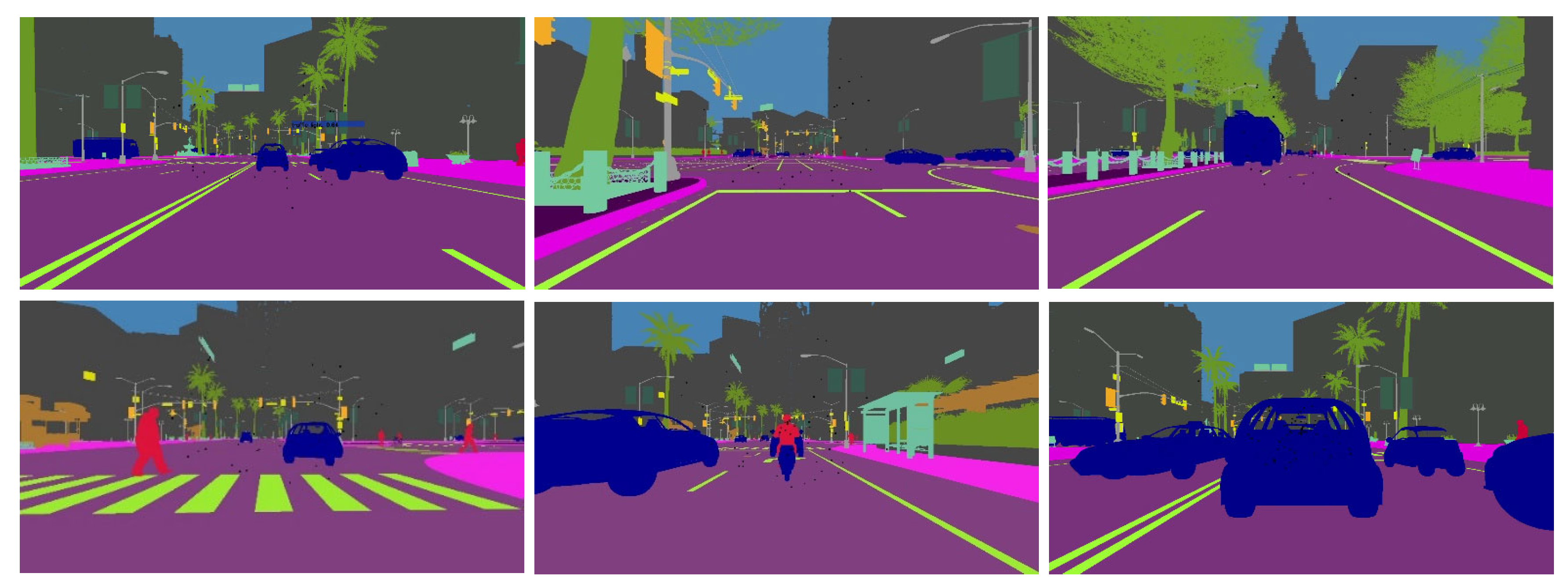
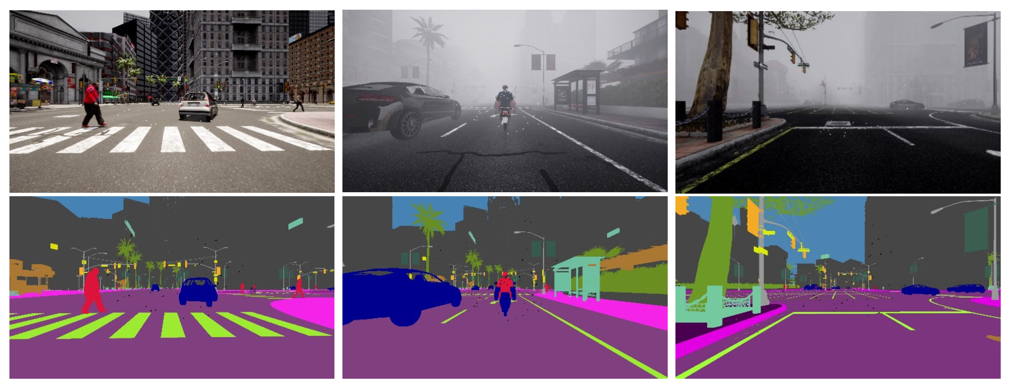
Figure 3 illustrates describing semantic labels obtained from the semantic segmentation camera in the CARLA simulator.
Alongside the camera and radar sensors, we attached semantic segmentation cameras to the ego vehicle to obtain semantic labels of the objects in its environment. The semantic segmentation camera presents each object in its field of vision with a distinct color corresponding to the predetermined 11 object categories. However, we make use of the seven common traffic participant (bicycle, bus, car, motorcycle, person, traffic light, and truck) labels in our work.
3.3. Object Detection Model
In this work, we employed our recently proposed CR-YOLOnet [
31], a deep learning-based camera-radar fusion network (CR-YOLOnet) for object detection with YOLOv5 as the baseline. Unlike the single-modal system used in the YOLOv5 baseline, the CR-YOLOnet takes input from both camera and radar sources as input. CR-YOLOnet uses two different CSPDarknet backbone networks to extract feature maps, one each for camera and radar. To further improve the network, the low-level feature information from the backbone network was sent to the feature fusion layers using two connections inspired by residual network concepts. These two connections aim to improve the network's gradient backpropagation while simultaneously limiting the amount of feature information loss for relatively small or distant objects obscured by fog. To detect multi-scale item sizes in foggy weather circumstances, we improved CR-YOLOnet with an attention framework. Attention modules are added into the fusion layers to draw greater emphasis to and improve the feature representation of the features that aid in object detection. The attention module additionally addresses the issue of high-level feature information loss. We used a similar experimental platform as this work and obtained our camera and radar data from CARLA simulator. For CR-YOLOnet training and testing, we used clear and foggy weather scenarios. With an accuracy (mAP at 0.50) of 0.849 and a speed of 69 fps, our small CR-YOLOnet model optimally maintained a balanced between accuracy and speed.
3.4. Object Tracking Method
The DeepSORT algorithm addresses the assignment problem of matching new detection measurements and predicted target states with the KF and Hungarian algorithms. The Hungarian algorithm with the Kalman filter algorithm provides a single-hypothesis tracking approach for moving targets. The Hungarian matching algorithm helps to match up new detections with the predicted tracks. There were three distinct phases to the tracks. (i) tentative tracks: for each unmatched detection, a new set of track propositions is generated and stored in the tracked list for further observations, (ii) confirmed tracks: detections that are matched successfully are kept in the track matrix, (iii) deleted tracks: detections that cannot be matched or are no longer appearing within a specified number of frames are deleted from the track list. In addition to the data association of position and motion information, the DeepSORT incorporates a CNN-based component that extracts and associates object appearance features to address ID switch problem
However, when it comes to tracking tasks under noisy situations such as fog, the network used for appearance feature extraction greatly influences the quality of the appearance feature information being extracted and, consequently, the tracking speed. The original feature extraction network is merely a very simple kind of convolution. As a result, targets with a high degree of appearance similarity on the detection frame are more likely to be mismatched with the wrong predictions. In addition, matching inaccuracies can occur when widely varied size objects are on the frame. Thus, there is a need for further refinement when it comes foggy weather applications.
In this work, our multi-object tracking technique is broken down into the following stages:
- (i)
The KF takes detection information (object bounding box provided by CR-YOLOnet) as the input measurement, then KF predicts the target object's future states (position) in the detection frame, and the prior estimate value of target object is estimated. Also, CR-YOLOnet extracts and saves the feature information of the target object on the detection frame.
- (ii)
The Hungarian algorithms employ the appearance feature and Mahalanobis distance to associate the target object in the detection frame and track. In the event that the association procedure generates a successful match, the system will proceed to a Kalman update and provide tracking results. However, if there is no match, cascade matching is employed to associate the unmatched detection frame and track. Each track has its own time update parameter, "time_since_update, " established throughout the cascade matching process. Since the tracks are sorted by "time_since_update", the unmatched detection frame is first associated with the track with the minimum "time_since_update" to prevent tracking failure while decreasing the frequency of ID switches.
- (iii)
To evaluate if the target object in the detection frame and the track have the same ID and are a match, we compute the percentage of overlapping areas to compute their similarity. If the similarity computation generates a successful match, the system will proceed to a Kalman update and provide tracking results. However, if there is no match for the subsequent five frames, the mismatched track will be associated with a new detection frame. The tracking result will be returned if the detection frame is found within the next five frames. The target is consequently deleted if no match is found after five frames.
To acquire the overall tracking result, it is necessary to modify and adapt the tracking trajectory obtained from the KF by repeating the three stages mentioned above. Allocating a new identifying ID or removing a set trajectory are the actions that must be taken once a detection frame is unable to match and track.
3.4.1. Kalman Filter Prediction of Target Object State
We employ a Kalman uniform velocity model for the object motion state estimation. Equations 1 and 2 describe the non-linear discrete-state space model. For the motion state of each target
, the target object state is set from the previous state
to the present state
, the measurement vector
is the target object detection result that consists of the bounding boxes co-ordinate (a, b) at the current scan
, and the process noise at scan
.
where is the state transition matrix, denotes the state white Gaussian process noise and is the estimated process error covariance matrix, is the measurement matrix, denotes the measurement of white Gaussian process noise, is the estimated measurement error covariance matrix, with an initial state , is the prior mean and is the initial covariance.
We represent the state of the target object by vector
and it can be expressed as follow:
where
is the bounding box co-ordinate of the target,
is the bounding box aspect ratio,
is the bounding box height,
represent the corresponding velocity information of
.
There are two primary parts to the Kalman filter. First, we make the predictions of the system state using the time update mathematical state model. Equations (4) and (5) describe the prediction of the future state of the target object and the future error covariance:
where is the prior estimate that describes the future state of the target object at scan , is the prior estimate of the future error covariance at scan , is the posterior estimate of the target object state at scan , is the posterior estimate of error covariance at scan .
Second, the predicted state values are compared to the measured state values to generate state estimation output. In equations (6), (7), and (8), we compute the Kalman gain, update the estimate using measurements
, and update the error covariance, respectively.
A state estimation output is generated from the adjusted difference between the predicted and observed states, considering the predicted noise and error in the system and the measurements. The generated state estimation output is fed into the mathematical state model described in equations (4) and (5) to predict the target object future state at the subsequent time update. Thus, the cycle starts all over again. The error between the real value and the observed value is minimized via the aforementioned iterative process, bringing the predicted value closer and closer to the real value until the optimal tracking outcome is attained.
3.4.2. Matching New Detections Measurements and Predicted Target States
The motion and appearance information matching is incorporated using (i) Mahalanobis distance and (ii) minimum cosine distance, respectively. Let and be the order number of the predicted target state and target bounding box detection.
- (i)
Mahalanobis distance:
The Mahalanobis distance (
) include the motion data by estimating the distance between the new target detections and predicted target states, and it can be calculated as follows:
where represents the bounding box detection, denotes the track in measurement space, denotes the projection of the predicted value of the track in the detection space, denotes the covariance matrix of the track in the measurement space.
With the KF's uncertainty estimation of the target state, the Mahalanobis distance computes the distance from the mean track to the detection's standard deviation. Then a threshold
described equation 2 is used to determine if the
track and
detection are related or not.
If the track and detection related, the threshold evaluates to . Otherwise, it is .
- (iI)
Appearance feature matching:
The appearance features of the target are disregarded while using Mahalanobis distance since it only considers the distance relationship between the detected target and the predicted target states. The appearance features are extracted using a simple convolutional neural network to incorporate the appearance metric. A total of two convolutional layers and six residual blocks makes up this network. Appearance feature descriptors
are extracted from each bounding box detection
using a simple convolutional neural network shown below. For each track
, all the matched appearance descriptors are stored in
. Hence the minimum cosine appearance
) distance between the
track and
detection can be calculated using equation 3.
Using the threshold
in equation 12, we can show whether
track and
detection in equation 11 are related. Similarly, if the
track and
detection related, the threshold evaluates
. Otherwise, it is
.
When the Mahalanobis distance is used in conjunction with the minimum value of the cosine distance, the DeepSORT algorithm's efficiency can be enhanced. The Mahalanobis distance includes details about object positions depending on the motion to address short-term prediction and matching. When the motion information is less reliable because of extended occlusions, the cosine distance considers appearance information that is important for re-establishing identities. Therefore, the fusion of Mahalanobis distance
and cosine distance
from equations 9 and 11, respectively is described using the weighted sum
in equation 13:
where
which is often set to 0.1 denotes the hyperparameter used for setting the weights of the Mahalanobis and cosine distances. In equation 14, a gated matrix helps to establish whether the association of metrics is related:
In addition the cascade-matching method is used to compare the predicted target's motion trajectory by KF and new target detection [
70]. A new measuring matrix is constructed using both target appearance features and velocity information to evaluate the degree of similarity between a detection and a trajectory. Although when compared to the SORT algorithm, the DeepSORT algorithm performs significantly better.
3.5. The Appearance Feature Extraction Model
As mentioned earlier, the appearance feature extraction model in the original DeepSORT employed merely convolution and pooling layer procedures. The feature map generated by the backbone network's output is prone to losing relevant details about the target object. For very small and distant targets, this leads to an incorrect knowledge of object appearance features. Multi-object tracking models notably need faster tracking speeds. In addition to tracking small and distant objects at a fast speed, extracting quality appearance features will enhance the DeepSORT algorithm to distinguish between objects with similar appearances and track them accurately. We proposed an appearance feature network to replace the basic convolutional neural network used for the appearance descriptor in the DeepSORT algorithm. Our deep appearance descriptor employs a CSPNet-based backbone for low-level feature extraction and an FPN-based neck for multi-scale level appearance feature fusion to address objects of varying sizes.
The cross-stage partial connection (CSP) is a method that was initially derived from CSPNet [
71] and is used to optimize complex computational processes. The CSP network can help to increase feature-learning capacity during training.
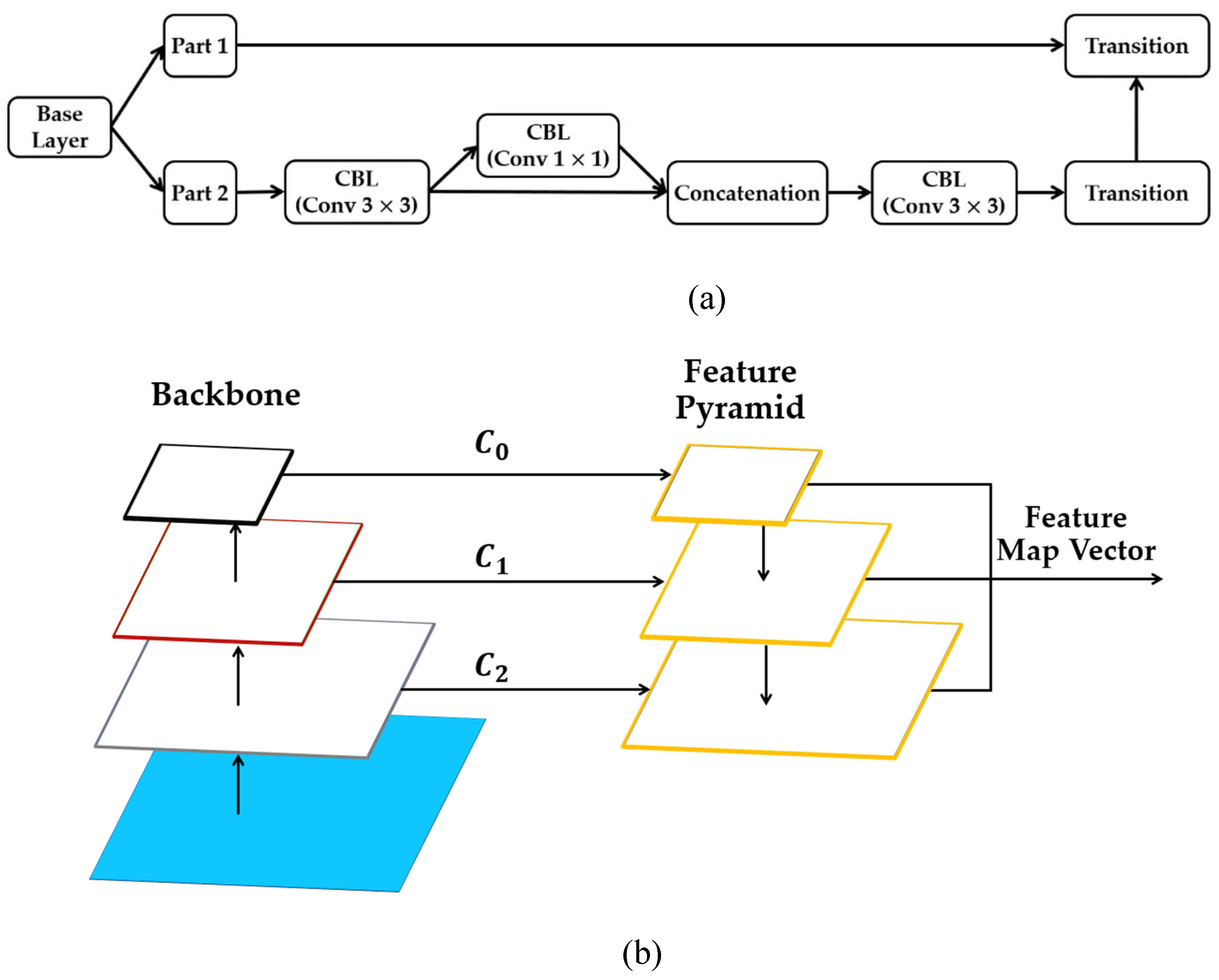
Figure 4(a) illustrates how a network can be "CSP-ize". The base layer's feature map is split into two components, the main component and a skip connection, combined by transition, concatenation, and transition to efficiently cut down on redundant gradient information. Because CSP-ization shortens gradient flow, therefore, CSP-ization increases accuracy and decreases inference time while making model scaling possible [
11]. As a result of scaling the model, the ability to detect objects of smaller sizes is made possible. Given the bigger size of the input network, the wider receptive field achieved by the CSP connection directly results from the higher number of convolutional layers.
The feature size plays a significant role in the representation of the target's feature information when performing feature extraction.
When generating the final feature map, the Feature Pyramid Network (FPN) [
72] shown in
Figure 4(b) aggregates features from several depths and layers. The final feature map includes a range of multi-layer semantic information due to the feature fusion that occurred at various levels. The feature pyramid network gets its name from its structure and shape, which are both reminiscent of pyramids. In FPN, the backbone networks are responsible for feature extraction, and the top-down fusion of feature maps is utilized to combine the resulting features
and
. Network structures of varying depths have varying degrees of accuracy when used to extract feature information from targets. Scale-dependent disparities in feature information during the matching phase can be mitigated by the use of fused object appearance feature information retrieved from several network depths. The FPN integrates a shallow feature extraction network for extracting spatial information with a deep feature extraction network for obtaining appearance feature information.
We adopted GhostNet, discussed in section 3.5.1, into our deep appearance descriptor to replace the traditional convolutional layers. We adopted a segmentation module discussed in section 3.5.2 to provide rich semantic information to the low-level appearance feature map using semantic labels.
3.5.1. GhostNet for an Improved Performance and Reduced Computational Complexity and Cost
The Ghost module was developed to take the place of the traditional convolutional layers in standard neural networks [
73]. The aim of the Ghost module, which is illustrated in
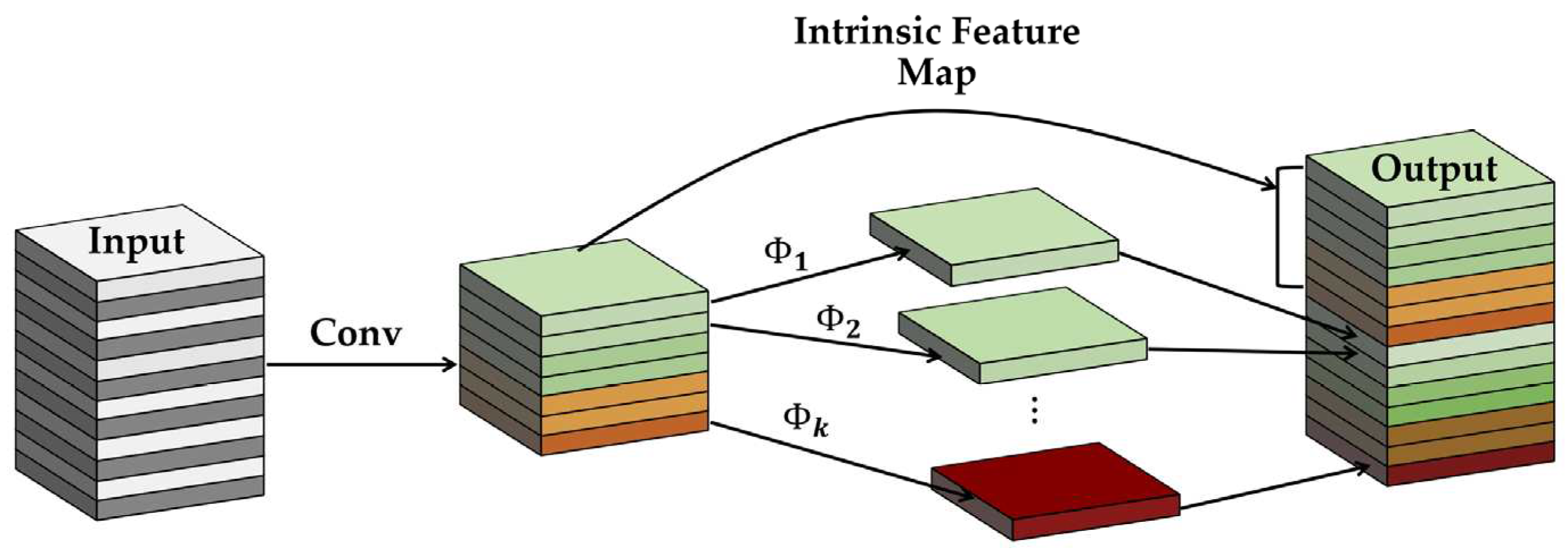
Figure 5, is: (i) to improve the performance of neural networks performance by generating more features, thus, improving the integrity of the feature extracted, (ii) to utilize a lesser number of parameters, thus, reducing computational complexities and cost without diminishing the output feature map. In the Ghost module, the conventional convolution process is divided into two separate steps. In the first step of the process, a conventional 1 x 1 convolution is performed on the input to acquire the required feature concentration. The second step involves performing a series of simple linear operations, such as layer-by-layer convolution on the intrinsic concentrated feature maps obtained from the prior step to produce additional feature maps.
Consider an input feature map
with
number of channels, height denoted by
and weight denoted by
, the procedure for generating n feature maps using conventional convolution can be expressed as:
where denotes the convolution kernels with size, denotes the bias term. is the convolution operation. Using convolution filter with kernel size, the output feature map is . The heights and widths of the output feature maps are denoted by and , respectively.
Because the number of filters and channels often needs to be quite high, the needed number of floating-number operations (FLOPs) may easily reach hundreds of thousands. The needed number of FLOPs for the conventional convolution process can be expressed as follows:
Assumptions can be made that the generated feature maps are "ghosts" of certain original feature maps that have been reshaped in a computationally cost-effective way. These assumptions can be made to prevent redundancy and similarities in the individual output feature maps generated by ordinary convolutional layers while exhausting a vast number of FLOPs and parameters. Equation 17 describes the ordinary convolution for creating the
intrinsic feature maps
such that
and
is the m convolution kernels of the size of
.
Applying a sequence of inexpensive linear operations to each intrinsic feature in
yields
ghost features, which may then be used to construct the necessary
feature maps as described in equation 18 and needed FLOPs in equation 19:
where denotes the ghost feature map generated by convolution kernel size of each linear operation excluding the last operation used retaining the maps of intrinsic features, is the intrinsic feature map in .
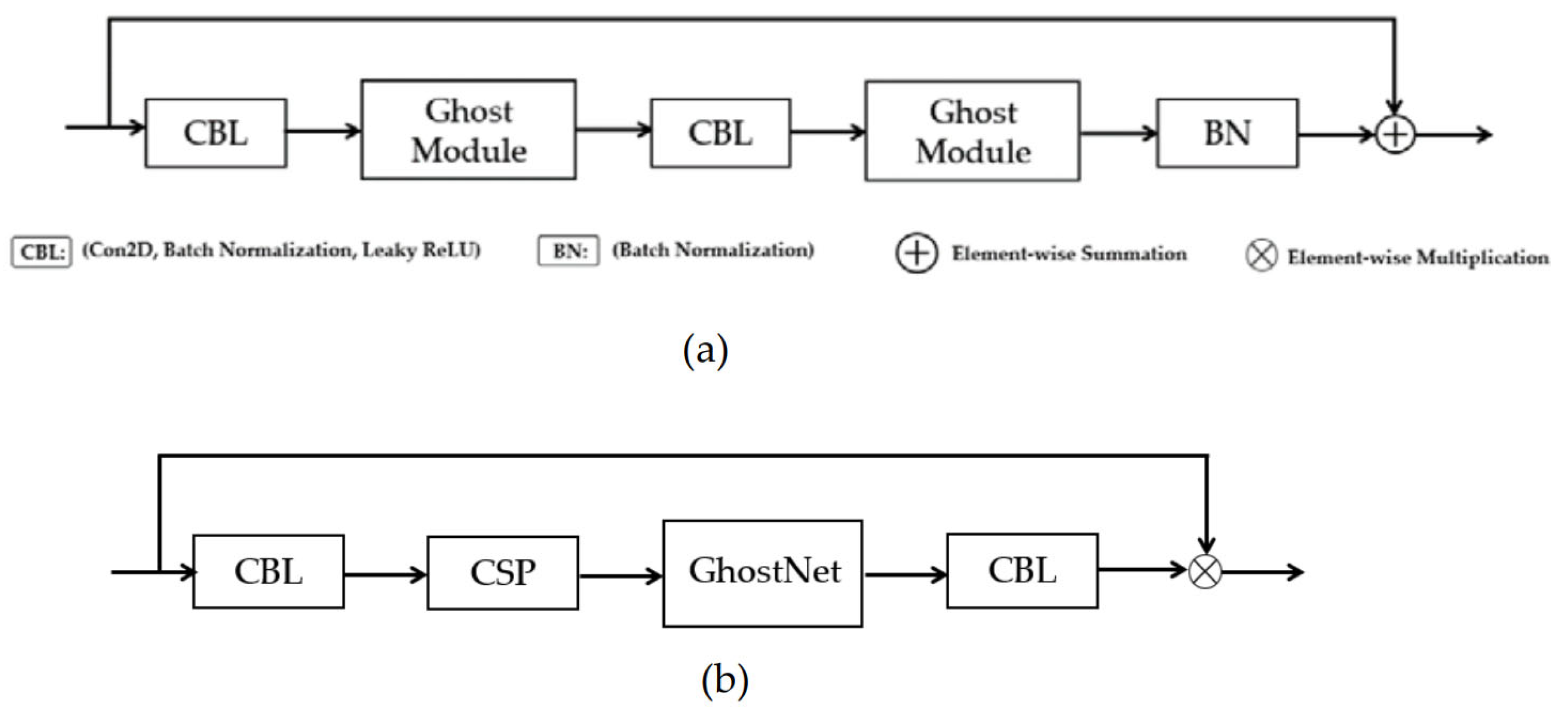
Figure 6(a) illustrates our GhostNet structure. The CBL module is made up of convolution, batch normalization, and the leaky ReLU activation function sub-modules. The Ghost module uses standard convolution to produce a portion of the original feature map. Next, it convolves each of these feature maps individually to get a portion of the associated feature map. And then adds the latter feature map with the first feature map. Our improved convolution operation called Ghost convolution consist of the CBL block, CSP block, and GhostNet block, as shown in
Figure 6(b).
3.5.2. Segmentation Module for an Improved Appearance Feature
We adopted the segmentation module (SM), which majorly is composed of atrous convolutional layers to add rich semantic information to the low-level appearance feature map generated using semantic labels from [
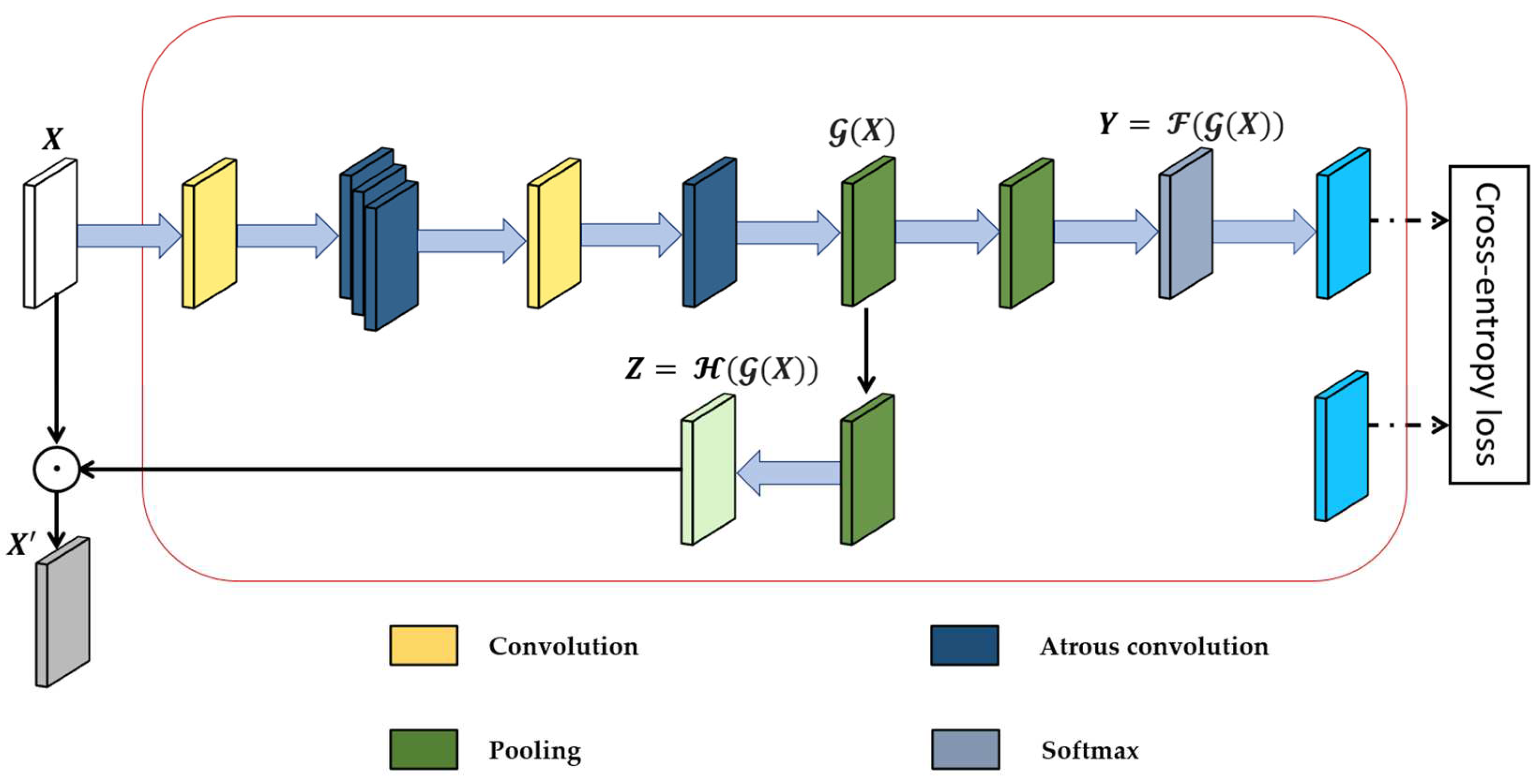
74]. The purpose of the semantic labels is to add their own robust semantic meaningful features to the low-level feature map extracted from the backbone network, as shown in
Figure 7. The goal of incorporating the segmentation module into the appearance feature extractor is to improve the integrity of appearance features and to be able to distinguish between objects of similar appearance in a noisy detection frame. Thus, mitigating the problem of mismatch between detection measurements and Kalman filter predictions under foggy weather conditions.
Several parameters make up the segmentation module. First, we consider a primary low-level input feature map
with
number of channels, height denoted by
and weight denoted by
, and semantic label (ground-truth)
such that
is the number of objects class in the label (in our case, we make use of 7 object classes). In equation 20, the intermediate feature map
is used to estimate the per-pixel segmentation prediction
, this is also known as
path. In addition, for the
path, the intermediate feature map
is employed to create a profound feature map
with semantic content as described in equation 21:
The element-wise multiplication of the primary low-level appearance feature map X and the semantically profound feature map Z activates
to give
. The activation process produces a map of low-level appearance features
which is a semantically activated appearance feature map.
does provide not only rudimentary visual patterns but also high-level semantic meaning. The cross-entropy loss function
of the segmentation module is given as:
where is the image, is semantic label and is the segmentation prediction.
4. Improved Deep Appearance Feature Extraction Network
4.1. The Architecture of Our Appearance Feature Extraction Network
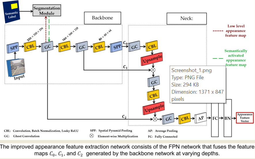
As previously mentioned, we chose CSPDarknet-based backbone with the intention of enhancing the functionality of the appearance feature extraction network illustrated in
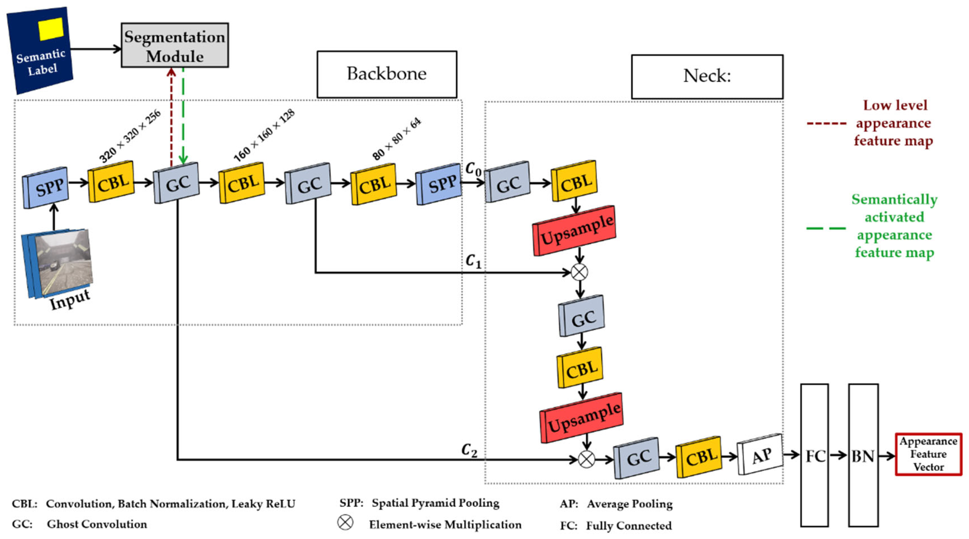
Figure 8. The ghost convolution block consists of the CBL block, CSP block and GhostNet block (see section 3.5.1). The goal of CSP block is to help improve the capacity of our networks to learn as many features as possible from an image during training. Introducing the GhostNet block helps to generate more features to enhance the integrity of the feature extracted while utilizing a lesser number of parameters to alleviate computational complexities and cost. To increase tracking accuracy and manage the autonomous driving task in dynamic and foggy weather environments, we integrate and fuse appearance features from several layers, resulting in a richer appearance feature vector.
Using the segmentation module from section 3.5.2, rich semantic information from semantic labels can help to improve the appearance feature vector generated by the appearance feature extraction network. In this work, we integrate the segmentation module into the backbone of CSPDarknet-based backbone and FPN-based neck because it is designed to generate multi-scale level feature maps including small, medium, and large size objects. In addition to the semantic label input, the segmentation module uses low-level appearance feature maps (denoted by the dark red square dot arrow in
Figure 8) generated in the backbone to understand semantic segmentation based on the influence of segmentation ground-truth. Thus, the segmentation module uses its own rich segmentation features to bolster the low-level features to produce low-level semantically activated appearance feature maps (denoted by the dark green long dash arrow in
Figure 8).
The low-level semantically activated appearance feature maps have the capability of acquiring not just the fundamental visual pattern of a target object but accurate semantic information associated with it.
We implemented spatial pyramid pooling (SPP) [
75] to (i) enhance the receptive field of our network, (ii) decouple the context features, and (iii) make it easier for the neck network to fuse appearance features from several layers. We introduced SPP at the beginning of the backbone network to prevent loss of resolution and noise in the input image that can occur if scaled and cropped. The SPP at the very end of the backbone network consists of three different pooling layers with sizes of 5×5, 7×7, and 13×13. To generate the many local features, SPP combines the results of the three pooling layers and feeds them as input to the subsequent convolutional module, where further feature learning is carried out.
,
, and
which are the extracted appearance feature maps from three different depths were fed into the FPN and fused. The appearance features generated by the
layer possesses rich and high-level semantic information that enhances the extraction of features from large target objects. The feature maps from the
layer is inadequate for feature extraction from small target objects. Despite the fact that
and
outputs may not have as much detail in their feature maps as
, they are excellent at extracting features from smaller target objects while still providing significant and useful positional information. The FPN network combines feature maps
,
, and
from the backbone network's output at varying depths, as shown in
Figure 8. After performing complete joining and batch normalizing, the resulting object appearance feature vector is acquired. The object appearance feature vector is used to determine an estimation of the extent to which the track's appearance is similar to the detection appearance. We performed the full cascading matching procedure using the motion information and the cost matrix, which is the estimation of appearance feature similarity between detection and tracks.
4.2. Training
Figure 9 illustrates samples of our CARLA dataset used for training our appearance feature extraction network in this work. The dataset includes both sunny and foggy conditions with RGB camera data in the top row and the corresponding semantic segmentation camera data in the second row, as shown in
Figure 9. The RGB data set serves as the input into the appearance feature network, while semantic segmentation serves as input (provides semantic labels) to the segmentation module. We make use of the seven common traffic participant (bicycle, bus, car, motorcycle, person, traffic light, and truck) labels in our work. There is a total of 18628 RGB pictures and with each having a corresponding semantic segmentation image. The training set consists of 80 percent of the images, and the remaining 20 percent is used for testing. The appearance feature extraction network was trained using both clear and foggy image datasets for 100 epochs with a batch size of
. To predict the spatial location of the tracked object, we used the CIoU loss function [
76] for bounding box regression described in our previous work [
25].
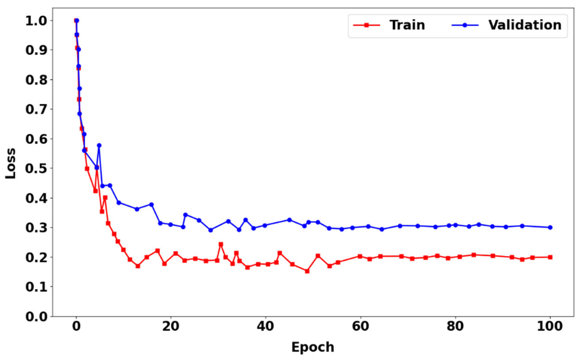
Figure 10 shows the training loss curve (red), which is the training phase, and the prediction loss curve (blue), which is the prediction phase of the appearance feature extraction network using CIoU loss with the segmentation module incorporated. In both the training and prediction phases, the loss curves decreased rapidly during the initial 15 epochs. Thus, the rate of loss begins to slow down in an unstable manner because of insufficient model accuracy at the start of the training phase. However, at the 60th epoch, both loss curves begin to flatten out and become stable until the 100th epoch.
5. Multi-Object Tracking Experimental Results and Discussion
5.1. Comparison of Multi-Object Tracking Performance using Our CARLA Dataset
Following the training phase of our appearance feature extraction network, the results of the training are then incorporated into our improved DeepSORT tracking model to evaluate the performance of our improved multi-target tracking algorithm. Throughout this section 5.1, we referred to our improved multi-target tracking algorithm using GIoU loss function [
77] with the segmentation module as "Ours(GIoU) with SM" and without the segmentation module as "Ours(GIoU) without SM". Similarly, we referred to our improved multi-target tracking algorithm using CIoU loss function [
76] with the segmentation module as "Ours(CIoU) with SM" and without the segmentation module as "Ours(CIoU) without SM". The following metrics serve as the basis for the evaluation [
10]:
The multi-object tracking accuracy (MOTA) describes the total tracking accuracy with respect to false positives (FP), false negatives (N) and identity switches (IDS), and it is expressed in equation 23.
The multi-object tracking precision (MOTP) describes the total tracking precision measured with respect to the amount of actual bounding box overlap with the predicted position, and it is expressed in equation 24.
where denotes the total number of matches at frame , is the distance between the predicted and the ground-truth bounding box, is the number of tracking targets. In addition, we performed evaluation using other metrics including mostly tracked (), mostly lost (). is used to describe the percentage of ground-truth tracks that do not switch labels for the majority (80%) of their existence. is used to describe the percentage of ground-truth tracks maintained for no more than 20% of their existence.
Table 1,
Table 2, and
Table 3 describe the multi-object tracking performance of Ours(CIoU) with and without SM and Ours(GIoU) with and without SM in clear-day, medium fog and heavy fog conditions, respectively. Under clear day weather condition in
Table 1, Ours(CIoU) with SM have MOTA of 74.86, MOTP of 84.21, MT of 43.40%, and a speed (FPS) of 68.34, which are higher than the other three models. In addition, Ours(CIoU) with SM has ML of 15.86% and IDS of 513, which is lower than the other three models. When compared to Ours(CIoU) without SM, the MOTA in Ours(CIoU) with SM increased by 4.30%, MOTP increased by 5.13%, MT increased by 7.83%, and a speed (FPS) increased by 8.58%. The ML and IDS were reduced by 12.16% and 14.25%, respectively.
When operating in medium fog conditions in
Table 2, Ours(CIoU) with SM has MOTA of 68.25, MOTP of 79.65, MT of 38.77%, and a speed (FPS) of 66.15, which are higher than the other three models. Moreover, Ours(CIoU) with SM has ML of 17.05% and IDS of 691, which is lower than the other three models. However, when compared to Ours(CIoU) without SM, the MOTA in Ours(CIoU) with SM increased by 5.10%, MOTP increased by 8.55%, MT increased by 14.38%, and a speed (FPS) increased by 11.01%. The ML and IDS were reduced by 15.31% and 17.01%, respectively.
In
Table 3, the heavy fog situation shows that Ours(CIoU) with SM has a MOTA of 66.14, MOTP of 75.78, MT of 36.80%, and a speed (FPS) of 64.88, all of which are greater than the other three models. In addition, Ours(CIoU) with SM has ML of 19.24% and IDS of 816, which is significantly lower than the other three models' respective values. When compared to Ours(CIoU) without SM, the MOTA in Ours(CIoU) with SM increased by 9.02%, MOTP increased by 7.43%, MT increased by 18.05% and the speed (FPS) increased by 15.32%. The ML and IDS were reduced by 15.57% and 21.09%, respectively.
In
Table 4, under clear day weather conditions, when compared to CR-YOLO + DeepSORT, the MOTA in Ours(CIoU) with SM increased by 8.58%, MOTP increased by 6.84%, MT increased by 13.85%, and a speed (FPS) increased by 11.59%. However, the ML and IDS were reduced by 22.58% and 37.99%, respectively. Compared to YOLOv5 + DeepSORT, the MOTA in Ours(CIoU) with SM increased by 18.12%, MOTP increased by 17.93%, MT increased by 37.19%, and a speed increased by 32.71%. However, the ML and IDS were reduced by 43.26% and 38.44%, respectively.
Under medium fog conditions in
Table 5, compared to CR-YOLO + DeepSORT, the MOTA in Ours (CIoU) with SM increased by 10.66%, the MOTP increased by 10.87%, MT increased by 16.38%, and the speed increased by 16.45%. Nonetheless, the ML and IDS in Ours (CIoU) with SM decreased by 24.60% and 38.06%, respectively. Compared to YOLOv5 + DeepSORT, the MOTA in Ours(CIoU) with SM increased by 24.13%, MOTP increased by 24.71%, MT increased by 43.27%, and the speed increased by 35.80. However, the ML and IDS decreased by 35.12% and 44.0%, respectively.
Under heavy fog conditions,
Table 6 shows that the MOTA in Ours (CIoU) with SM increased by 16.17%, the MOTP increased by 17.99%, MT increased by 23.27%, and the speed increased by 23.39% in comparison to CR-YOLO + DeepSORT. However, the ML and IDS decreased by 27.54% and 40.78%, respectively. Compared to YOLOv5 + DeepSORT, the MOTA in Ours (CIoU) with SM increased by 35.15%, the MOTP increased by 32.65%, MT saw an increase of 48.72%, and the speed saw an increase of 37.65%. However, the ML and IDS decreased by 41.65% and 46.81%, respectively, when compared to YOLOV5 + DeepSORT. This implies that employing the segmentation module and CIoU loss function efficiently improve our proposed model's object tracking capability in foggy and clear weather conditions.
5.2. Qualitative Results of Multi-Object Tracking Performance on Our CARLA Dataset
In this section, we present a comparison of the qualitative results of CR-YOLO + Ours(CIoU) with SM, CR-YOLO + Ours(GIoU) with SM, CR-YOLO + DeepSORT on our CARLA dataset. Throughout this section 5.2, CR-YOLO + Ours(CIoU) with SM, CR-YOLO + Ours(GIoU) with SM, and CR-YOLO + DeepSORT are referenced as Ours(CIoU), Ours(GIoU), and CR-YOLO DeepSORT respectively.
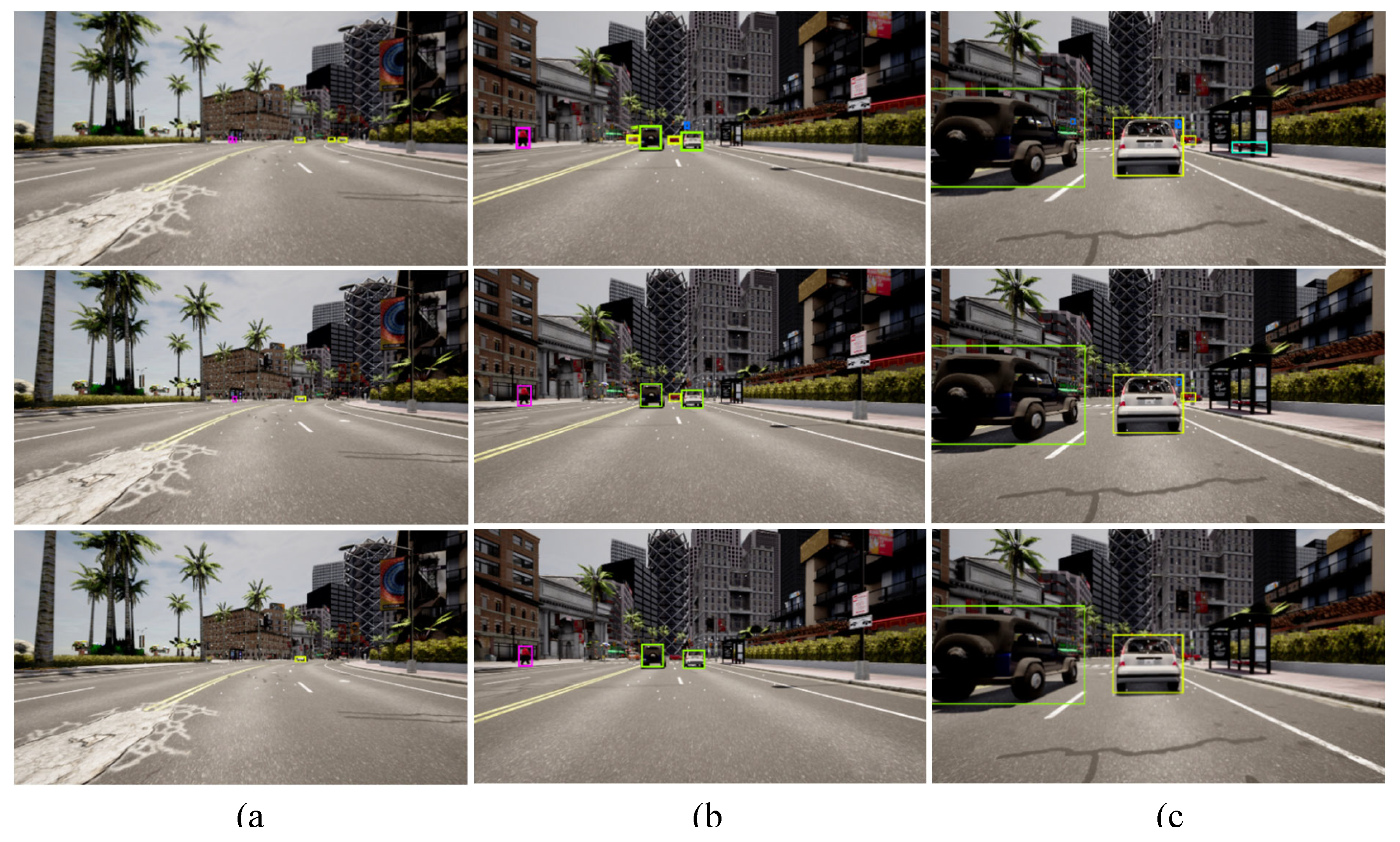
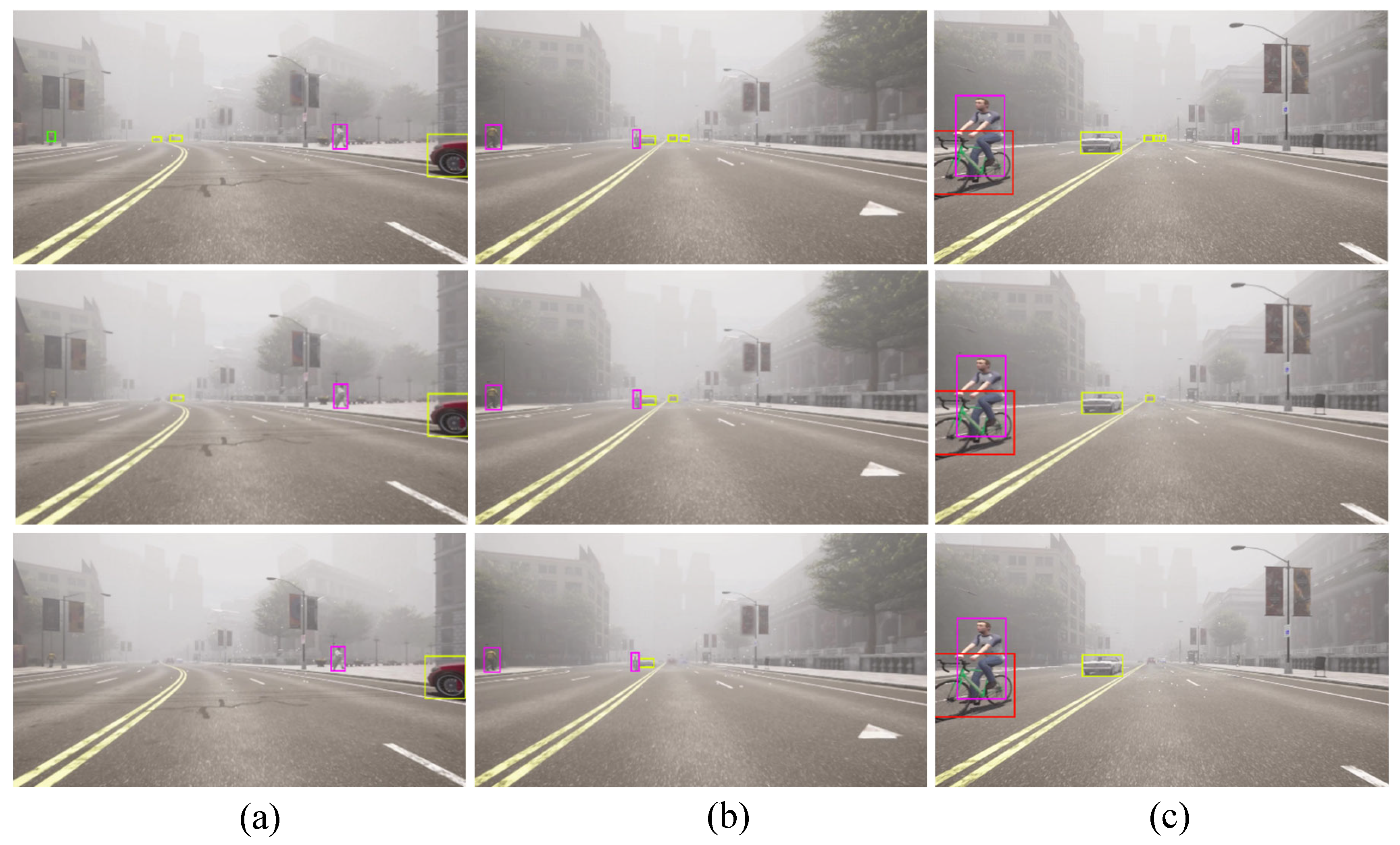
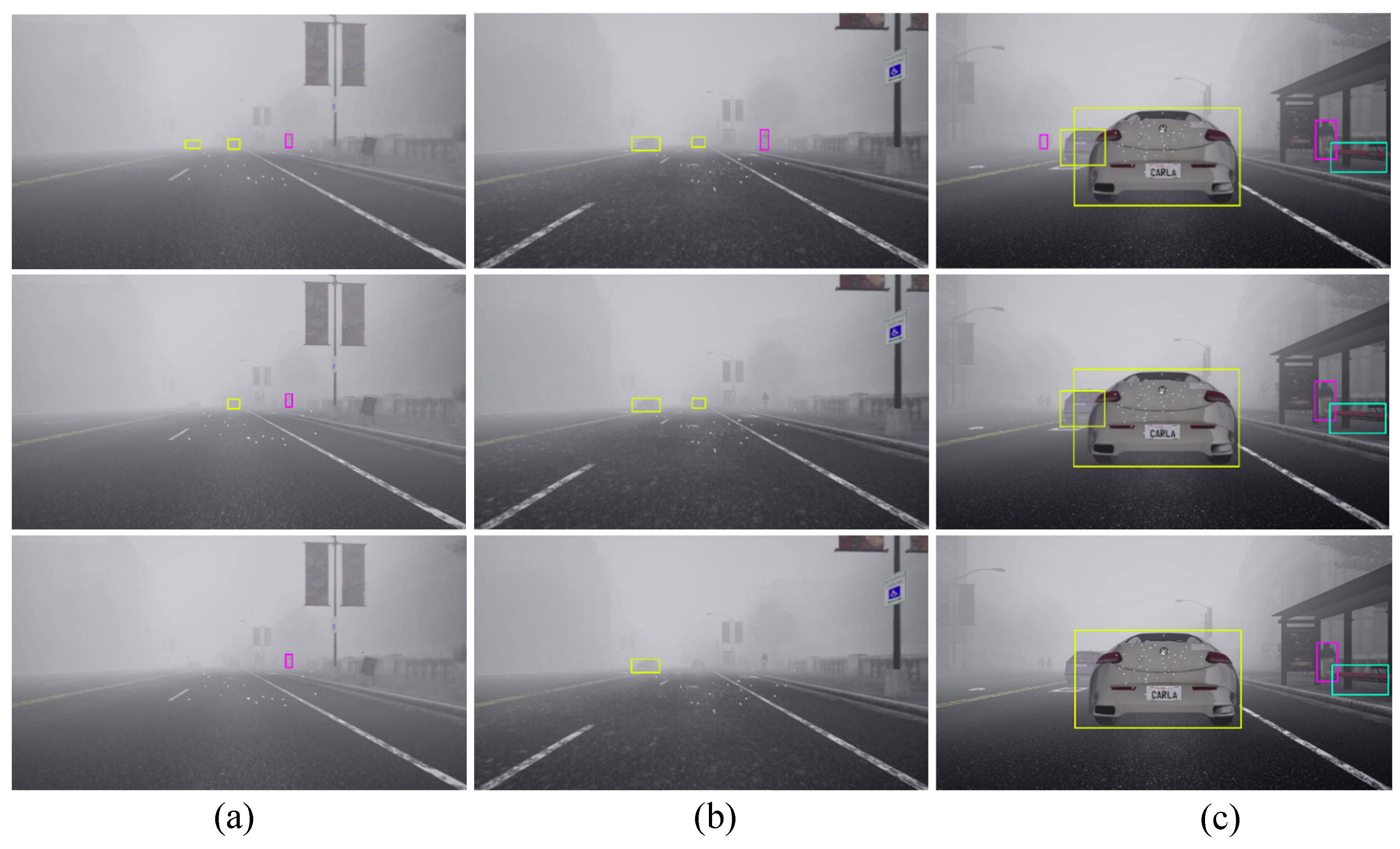
As previously mentioned in section 3.4, if the similarity computation between the target object in the detection frame and the track generates a successful match, the system will proceed to a Kalman update and provide tracking results. If no match is found after five frames, the target is marked as untrackable and consequently deleted. This implies that, even though the CR-YOLO algorithm is efficient in detecting both small and distant target objects, it is up to the tracking module to generate a successful match within the first five frames for tracking results to continue. We compare Ours(CIoU) displayed in row 1, Ours(GIoU) displayed in row 2, and CR-YOLO + DeepSORT displayed in row 3 under clear weather conditions (
Figure 11), medium fog weather conditions (
Figure 12), and heavy fog weather conditions (
Figure 13).
In Figures 11(a), 12(a), and 13(a), several distant and small objects were detected and tracked. However, these objects were tracked until they were closed and became medium size in Figures 11(b), 12(b), and 13(b) and larger size in Figures 11(c), 12(c), and 13(c). Ours(CIoU) performed better than Ours(GIoU) and DeepSORT tracking modules, especially regarding distant and small objects. Ours(CIoU) successfully generated, maintained, and matched more tracks than Ours(GIoU) and DeepSORT. For instance, in
Figure 11(a), Ours(CIoU) confirmed and maintained four tracks compared to two tracks in Ours(GIoU) and one track in DeepSORT.
Similarly, in
Figure 12(a), Ours(CIoU) confirmed and maintained 5 tracks compared to 3 tracks in Ours(GIoU) and 2 tracks in DeepSORT. In
Figure 13(a), Ours(CIoU) confirmed and maintained 3 tracks compared to 2 tracks in Ours(GIoU) and 1 track in DeepSORT. Similarly, for medium-sized objects, in
Figure 11(b), Ours(CIoU) confirmed and maintained 6 tracks compared to 4 tracks in Ours(GIoU) and 3 tracks in DeepSORT. In
Figure 12(b), Ours(CIoU) maintained 5 tracks compared to 4 tracks in Ours(GIoU) and 3 tracks in DeepSORT.
Ours(CIoU) successfully handled MOT even when there was a variation of target sizes in the detection frame in all three weather scenarios. In
Figure 11(c), while tracking large size objects, distant vehicles and traffic lights that appeared small were tracked simultaneously by Ours(CIoU) and Ours(GIoU), unlike the CR-YOLO DeepSORT that tracked the larger objects only. However, in
Figure 13(c), under heavy fog conditions, only Ours(CIoU) was able to track the distant and small size pedestrians, unlike Ours(GIoU) and CR-YOLO DeepSORT, which tracked the larger objects only. Obviously, the CR-YOLO DeepSORT performed better in clear weather conditions than in medium and heavy fog conditions. For instance, in
Figure 13(c), DeepSORT could not confirm and track the sport utility vehicle due to occlusion and atmospheric scattering. However, despite the problem of occlusion and atmospheric scattering, both Ours(CIoU) and Ours(GIoU) successfully maintained the object's identity for a more extended period.
In all three weather conditions, fusing the appearance feature map at three different depth levels and with the segmentation module gave Ours(CIoU) and Ours(GIoU) better performance leverage over the CR-YOLO DeepSORT. Ours(CIoU) performed better than Ours(GIoU) due to the CIoU loss function that not only considers non-overlapping regions between the actual and ground-truth frames but also uses the weight function. The weight function is a trade-off parameter that gives the overlap region factor a higher priority for regression. CIoU also measures the consistency or similarity of the aspect ratio between the bounding boxes. Thus, the ability of the tracking model to efficiently generate and match tracks is essential for critical safety systems such as autonomous driving.
6. Conclusion
An improved multi-object tracking model based on the DeepSORT algorithm was presented in this paper. When fog is present, it can be difficult to detect or track distant or small objects in an autonomous driving environment. As an example of a safety-critical situation, an autonomous driving environment necessitates for a higher tracking speed in multi-object tracking models. Object appearance features were extracted using a primitive neural network in the original DeepSORT method. Therefore, the resulting feature map often omits important information about the target being matched with a specific detection. Consequently, identity switches and track failures are more likely to occur when matching objects that look quite similar in the detection frame. Errors in matching can also arise if items of varying sizes are included in the detection frame.
Nevertheless, we used our camera-radar fusion network during the detection phase to increase both the speed with which objects could be detected and the accuracy with which they could be tracked when visibility was extremely low. Instead of using a standard convolutional neural network, we proposed a more robust appearance feature network. We incorporated GhostNet to take the role of the standard convolutional layers to produce more features and lower computational difficulties and costs while improving tracking speed without reducing the output feature maps. We also included a segmentation module (SM) and gave it the semantic labels from the input frame to enrich the feature maps for the low-level appearance with rich semantic information. Distinguishing between items that appear identical in a noisy background, like fog, is made easier with the addition of rich semantic information. To deal with the problem of variation in object in size on the detection frame, the appearance features were fused at three different depths. Our proposed MOT method performed better than YOLOv5 + DeepSORT, such that under heavy fog conditions, the multi-object tracking accuracy (MOTA) increased by 35.15%, the multi-object tracking precision (MOTP) increased by 32.65%, the speed increased by 37.65%, and identity switches (IDS) decreased by 46.81%.
Author Contributions
Conceptualization, I.O. and S.B.; methodology, I.O.; software, I.O.; writing—original draft preparation, I.O.; writing—review and editing, I.O.; supervision and review, S.B. All authors have read and agreed to the published version of the manuscript.
Funding
This research received no external funding.
Institutional Review Board Statement
Not applicable.
Informed Consent Statement
Not applicable.
Conflicts of Interest
The authors declare no conflict of interest.
References
- Nabati, M.R. Sensor Fusion for Object Detection and Tracking in Autonomous. Vehicles. Dissertation, University of Tennessee, Knoxville, Knoxville, 2021. [Google Scholar]
- Zhang, X.-Q.; Jiang, R.-H.; Fan, C.-X.; Tong, T.-Y.; Wang, T.; Huang, P.-C. Advances in Deep Learning Methods for Visual Tracking: Literature Review and Fundamentals. International Journal of Automation and Computing 2021, 18, 311–333. [Google Scholar] [CrossRef]
- Wu, Z.; Li, F.; Zhu, Y.; Lu, K.; Wu, M. Design of a Robust System Architecture for Tracking Vehicle on Highway Based on Monocular Camera. Sensors 2022, 22, 3359. [Google Scholar] [CrossRef] [PubMed]
- Jang, J.; Seon, M.; Choi, J. Lightweight Indoor Multi-Object Tracking in Overlapping FOV Multi-Camera Environments. Sensors 2022, 22, 5267. [Google Scholar] [CrossRef]
- Li, J.; Ding, Y.; Wei, H.-L.; Zhang, Y.; Lin, W. SimpleTrack: Rethinking and Improving the JDE Approach for Multi-Object Tracking. Sensors 2022, 22, 5863. [Google Scholar] [CrossRef] [PubMed]
- Zhang, J.; Hu, T.; Shao, X.; Xiao, M.; Rong, Y.; Xiao, Z. Multi-Target Tracking Using Windowed Fourier Single-Pixel Imaging. Sensors 2021, 21, 7934. [Google Scholar] [CrossRef]
- Diab, M.S.; Elhosseini, M.A.; El-Sayed, M.S.; Ali, H.A. Brain Strategy Algorithm for Multiple Object Tracking Based on Merging Semantic Attributes and Appearance Features. Sensors 2021, 21, 7604. [Google Scholar] [CrossRef]
- Bar-Shalom, Y.; Daum, F.; Huang, J. The probabilistic data association filter. IEEE Control Systems Magazine 2009, 29, 82–100. [Google Scholar] [CrossRef]
- Bewley, A.; Ge, Z.; Ott, L.; Ramos, F.; Upcroft, B. Simple online and realtime tracking. In Proceedings of the 2016 IEEE international conference on image processing (ICIP); 2016; pp. 3464–3468. [Google Scholar]
- Wojke, N.; Bewley, A.; Paulus, D. Simple online and realtime tracking with a deep association metric. In Proceedings of the 2017 IEEE international conference on image processing (ICIP); 2017; pp. 3645–3649. [Google Scholar]
- Parico, A.I.B.; Ahamed, T. Real Time Pear Fruit Detection and Counting Using YOLOv4 Models and Deep SORT. Sensors 2021, 21, 4803. [Google Scholar] [CrossRef]
- Qiu, Z.; Zhao, N.; Zhou, L.; Wang, M.; Yang, L.; Fang, H.; He, Y.; Liu, Y. Vision-Based Moving Obstacle Detection and Tracking in Paddy Field Using Improved Yolov3 and Deep SORT. Sensors 2020, 20, 4082. [Google Scholar] [CrossRef] [PubMed]
- Zhao, Y.; Zhou, X.; Xu, X.; Jiang, Z.; Cheng, F.; Tang, J.; Shen, Y. A Novel Vehicle Tracking ID Switches Algorithm for Driving Recording Sensors. Sensors 2020, 20, 3638. [Google Scholar] [CrossRef]
- Pereira, R.; Carvalho, G.; Garrote, L.; Nunes, U.J. Sort and Deep-SORT Based Multi-Object Tracking for Mobile Robotics: Evaluation with New Data Association Metrics. Applied Sciences 2022, 12, 1319. [Google Scholar] [CrossRef]
- Lee, S.; Kim, E. Multiple object tracking via feature pyramid siamese networks. IEEE access 2018, 7, 8181–8194. [Google Scholar] [CrossRef]
- Jin, J.; Li, X.; Li, X.; Guan, S. Online multi-object tracking with Siamese network and optical flow. In Proceedings of the 2020 IEEE 5th International Conference on Image, 2020, Vision and Computing (ICIVC); pp. 193–198.
- De Ponte Müller, F. Survey on Ranging Sensors and Cooperative Techniques for Relative Positioning of Vehicles. 2017, 17, 271.
- De-Las-Heras, G.; Sánchez-Soriano, J.; Puertas, E. Advanced Driver Assistance Systems (ADAS) Based on Machine Learning Techniques for the Detection and Transcription of Variable Message Signs on Roads. Sensors (Basel) 2021, 21, 5866. [Google Scholar] [CrossRef]
- Fayyad, J.; Jaradat, M.A.; Gruyer, D.; Najjaran, H. Deep Learning Sensor Fusion for Autonomous Vehicle Perception and Localization: A Review. Sensors 2020, 20, 4220. [Google Scholar] [CrossRef]
- Al-Haija, Q.A.; Gharaibeh, M.; Odeh, A. Detection in Adverse Weather Conditions for Autonomous Vehicles via Deep Learning. AI 2022, 3, 303–317. [Google Scholar] [CrossRef]
- Bijelic, M.; Gruber, T.; Mannan, F.; Kraus, F.; Ritter, W.; Dietmayer, K.; Heide, F. Seeing through fog without seeing fog: Deep multimodal sensor fusion in unseen adverse weather. In Proceedings of the Proceedings of the IEEE/CVF Conference on Computer Vision and Pattern Recognition, 2020; pp. 11682–11692.
- Hasirlioglu, S.; Riener, A. Challenges in Object Detection Under Rainy Weather Conditions. Cham, 2019; pp. 53-65.
- Song, R.; Wetherall, J.; Maskell, S.; Ralph F., J. Weather Effects on Obstacle Detection for Autonomous Car. In Proceedings of the International Conference on Vehicle Technology and Intelligent Transport Systems; 2020. [Google Scholar]
- Zang, S.; Ding, M.; Smith, D.; Tyler, P.; Rakotoarivelo, T.; Kaafar, M.A. The Impact of Adverse Weather Conditions on Autonomous Vehicles: How Rain, Snow, Fog, and Hail Affect the Performance of a Self-Driving Car. IEEE Vehicular Technology Magazine 2019, 14, 103–111. [Google Scholar] [CrossRef]
- Ogunrinde, I.; Bernadin, S. A Review of the Impacts of Defogging on Deep Learning-Based Object Detectors in Self-Driving Cars. In Proceedings of the SoutheastCon 2021, 2021, 10-13 March 2021; pp. 01–08. [Google Scholar]
- Tan, R.T. Visibility in bad weather from a single image. In Proceedings of the 2008 IEEE Conference on Computer Vision and Pattern Recognition; 2008; pp. 1–8. [Google Scholar]
- Choi, W.Y.; Yang, J.H.; Chung, C.C. Data-Driven Object Vehicle Estimation by Radar Accuracy Modeling with Weighted Interpolation. 2021, 21, 2317.
- Nabati, R.; Qi, H.J.A. Radar-Camera Sensor Fusion for Joint Object Detection and Distance Estimation in Autonomous Vehicles. 2020, abs/2009.08428.
- Chang, S.; Zhang, Y.; Zhang, F.; Zhao, X.; Huang, S.; Feng, Z.; Wei, Z. Spatial Attention Fusion for Obstacle Detection Using MmWave Radar and Vision Sensor. Sensors 2020, 20, 956. [Google Scholar] [CrossRef]
- Zhang, X.; Zhou, M.; Qiu, P.; Huang, Y.; Li, J. Radar and vision fusion for the real-time obstacle detection and identification. Industrial Robot: the international journal of robotics research and application 2019, 46, 391–395. [Google Scholar] [CrossRef]
- Ogunrinde, I.; Bernadin, S. Deep Camera-Radar Fusion with Attention Framework for Autonomous Vehicle Vision in Foggy Weather Conditions. Preprints.org 2023, 2023052180. [Google Scholar] [CrossRef] [PubMed]
- Dosovitskiy, A.; Ros, G.; Codevilla, F.; Lopez, A.; Koltun, V.J.a.p.a. CARLA: An open urban driving simulator. 2017.
- Ahmed, M.; Hashmi, K.A.; Pagani, A.; Liwicki, M.; Stricker, D.; Afzal, M.Z. Survey and Performance Analysis of Deep Learning Based Object Detection in Challenging Environments. 2021, 21, 5116.
- Alzubaidi, L.; Zhang, J.; Humaidi, A.J.; Al-Dujaili, A.; Duan, Y.; Al-Shamma, O.; Santamaría, J.; Fadhel, M.A.; Al-Amidie, M.; Farhan, L. Review of deep learning: concepts, CNN architectures, challenges, applications, future directions. Journal of Big Data 2021, 8, 53. [Google Scholar] [CrossRef] [PubMed]
- Jiao, L.; Zhang, F.; Liu, F.; Yang, S.; Li, L.; Feng, Z.; Qu, R. A Survey of Deep Learning-Based Object Detection. IEEE Access 2019, 7, 128837–128868. [Google Scholar] [CrossRef]
- Abdu, F.J.; Zhang, Y.; Fu, M.; Li, Y.; Deng, Z. Application of Deep Learning on Millimeter-Wave Radar Signals: A Review. 2021, 21, 1951.
- Krizhevsky, A.; Sutskever, I.; Hinton, G.E. ImageNet classification with deep convolutional neural networks. In Proceedings of the CACM; 2017. [Google Scholar]
- Liu, W.; Anguelov, D.; Erhan, D.; Szegedy, C.; Reed, S.; Fu, C.-Y.; Berg, A.C. Ssd: Single shot multibox detector. In Proceedings of the European conference on computer vision; 2016; pp. 21–37. [Google Scholar]
- Redmon, J.; Divvala, S.; Girshick, R.; Farhadi, A. You only look once: Unified, real-time object detection. In Proceedings of the Proceedings of the IEEE conference on computer vision and pattern recognition, 2016; pp. 779–788.
- Redmon, J.; Farhadi, A. YOLO9000: better, faster, stronger. In Proceedings of the Proceedings of the IEEE conference on computer vision and pattern recognition, 2017; pp. 7263–7271.
- Redmon, J.; Farhadi, A. Yolov3: An incremental improvement. arXiv preprint arXiv:1804.02767 2018.
- Benjdira, B.; Khursheed, T.; Koubaa, A.; Ammar, A.; Ouni, K. Car detection using unmanned aerial vehicles: Comparison between faster r-cnn and yolov3. In Proceedings of the 2019 1st International Conference on Unmanned Vehicle Systems-Oman (UVS); 2019; pp. 1–6. [Google Scholar]
- Bochkovskiy, A.; Wang, C.-Y.; Liao, H.-Y.M. Yolov4: Optimal speed and accuracy of object detection. arXiv preprint arXiv:2004.10934 2020.
- Jocher, G.; Nishimura, K.; Mineeva, T.; Vilariño, R. YOLOv5 (2020). GitHub repository: https://github. com/ultralytics/yolov5 2020.
- Girshick, R.; Donahue, J.; Darrell, T.; Malik, J. Rich feature hierarchies for accurate object detection and semantic segmentation. In Proceedings of the Proceedings of the IEEE conference on computer vision and pattern recognition, 2014; pp. 580–587.
- Girshick, R. Fast R‐CNN. In Proceedings of the 2015 IEEE International Conference on Computer Vision
(ICCV), 7‐13 Dec. 2015, 2015; pp. 1440‐1448.
- He, K.; Gkioxari, G.; Dollár, P.; Girshick, R. Mask R‐CNN. In Proceedings of the 2017 IEEE International
Conference on Computer Vision (ICCV), 22‐29 Oct. 2017, 2017; pp. 2980‐2988.
- Ren, S.; He, K.; Girshick, R.; Sun, J. Faster R-CNN: Towards Real-Time Object Detection with Region Proposal Networks. IEEE Transactions on Pattern Analysis and Machine Intelligence 2017, 39, 1137–1149. [Google Scholar] [CrossRef]
- Chadwick, S.; Maddern, W.; Newman, P. Distant vehicle detection using radar and vision. In Proceedings of the 2019 International Conference on Robotics and Automation (ICRA); 2019; pp. 8311–8317. [Google Scholar]
- John, V.; Nithilan, M.; Mita, S.; Tehrani, H.; Sudheesh, R.; Lalu, P. So-net: Joint semantic segmentation and obstacle detection using deep fusion of monocular camera and radar. In Proceedings of the Pacific-Rim Symposium on Image and Video Technology; 2019; pp. 138–148. [Google Scholar]
- Meyer, M.; Kuschk, G. Deep learning based 3d object detection for automotive radar and camera. In Proceedings of the 2019 16th European Radar Conference (EuRAD); 2019; pp. 133–136. [Google Scholar]
- Nobis, F.; Geisslinger, M.; Weber, M.; Betz, J.; Lienkamp, M. A deep learning-based radar and camera sensor fusion architecture for object detection. In Proceedings of the 2019 Sensor Data Fusion: Trends, Solutions, 2019, Applications (SDF); pp. 1–7.
- Yoo, H.; Kim, K.; Byeon, M.; Jeon, Y.; Choi, J.Y. Online Scheme for Multiple Camera Multiple Target Tracking Based on Multiple Hypothesis Tracking. IEEE Transactions on Circuits and Systems for Video Technology 2017, 27, 454–469. [Google Scholar] [CrossRef]
- Sheng, H.; Chen, J.; Zhang, Y.; Ke, W.; Xiong, Z.; Yu, J. Iterative Multiple Hypothesis Tracking With Tracklet-Level Association. IEEE Transactions on Circuits and Systems for Video Technology 2019, 29, 3660–3672. [Google Scholar] [CrossRef]
- Reid, D. An algorithm for tracking multiple targets. IEEE transactions on Automatic Control 1979, 24, 843–854. [Google Scholar] [CrossRef]
- Chen, L.; Ai, H.; Zhuang, Z.; Shang, C. Real-time multiple people tracking with deeply learned candidate selection and person re-identification. In Proceedings of the 2018 IEEE international conference on multimedia and expo (ICME); 2018; pp. 1–6. [Google Scholar]
- Mozhdehi, R.J.; Medeiros, H. Deep convolutional particle filter for visual tracking. In Proceedings of the
2017 IEEE International Conference on Image Processing (ICIP), 17‐20 Sept. 2017, 2017; pp. 3650‐3654.
- Kalman, R.E. A new approach to linear filtering and prediction problems. 1960.
- Kuhn, H.W. The Hungarian method for the assignment problem. Naval research logistics quarterly 1955, 2, 83–97. [Google Scholar] [CrossRef]
- Chen, J.; Xi, Z.; Wei, C.; Lu, J.; Niu, Y.; Li, Z. Multiple Object Tracking Using Edge Multi-Channel Gradient Model With ORB Feature. IEEE Access 2021, 9, 2294–2309. [Google Scholar] [CrossRef]
- He, J.; Huang, Z.; Wang, N.; Zhang, Z. Learnable graph matching: Incorporating graph partitioning with deep feature learning for multiple object tracking. In Proceedings of the Proceedings of the IEEE/CVF conference on computer vision and pattern recognition, 2021; pp. 5299–5309.
- Lucas, B.D.; Kanade, T. An iterative image registration technique with an application to stereo vision; Vancouver: 1981; Volume 81.
- Zhou, Y.; Liu, L.; Zhao, H.; López-Benítez, M.; Yu, L.; Yue, Y. Towards Deep Radar Perception for Autonomous Driving: Datasets, Methods, and Challenges. Sensors 2022, 22, 4208. [Google Scholar] [CrossRef]
- Caesar, H.; Bankiti, V.; Lang, A.H.; Vora, S.; Liong, V.E.; Xu, Q.; Krishnan, A.; Pan, Y.; Baldan, G.; Beijbom,
O. nuScenes: A Multimodal Dataset for Autonomous Driving. 2020 IEEE/CVF Conference on Computer Vision
and Pattern Recognition (CVPR) 2020, 11618‐11628.
- Barnes, D.; Gadd, M.; Murcutt, P.; Newman, P.; Posner, I. The oxford radar robotcar dataset: A radar extension to the oxford robotcar dataset. In Proceedings of the 2020 IEEE International Conference on Robotics and Automation (ICRA); 2020; pp. 6433–6438. [Google Scholar]
- Kim, G.; Park, Y.S.; Cho, Y.; Jeong, J.; Kim, A. MulRan: Multimodal Range Dataset for Urban Place Recognition. In Proceedings of the 2020 IEEE International Conference on Robotics and Automation (ICRA), 2020, 31 May-31 Aug. 2020; pp. 6246–6253. [Google Scholar]
- Sheeny, M.; De Pellegrin, E.; Mukherjee, S.; Ahrabian, A.; Wang, S.; Wallace, A. RADIATE: A radar dataset for automotive perception in bad weather. In Proceedings of the 2021 IEEE International Conference on Robotics and Automation (ICRA); 2021; pp. 1–7. [Google Scholar]
- Meyer, M.; Kuschk, G. Automotive radar dataset for deep learning based 3d object detection. In Proceedings of the 2019 16th european radar conference (EuRAD); 2019; pp. 129–132. [Google Scholar]
- Dosovitskiy, A.; Ros, G.; Codevilla, F.; Lopez, A.; Koltun, V. CARLA: An open urban driving simulator. In Proceedings of the Conference on robot learning; 2017; pp. 1–16. [Google Scholar]
- Liu, H.; Pei, Y.; Bei, Q.; Deng, L. Improved DeepSORT Algorithm Based on Multi-Feature Fusion. Applied System Innovation 2022, 5, 55. [Google Scholar] [CrossRef]
- Wang, C.-Y.; Liao, H.-Y.M.; Wu, Y.-H.; Chen, P.-Y.; Hsieh, J.-W.; Yeh, I.-H. CSPNet: A new backbone that can enhance learning capability of CNN. In Proceedings of the Proceedings of the IEEE/CVF conference on computer vision and pattern recognition workshops, 2020; pp. 390–391.
- Lin, T.-Y.; Dollár, P.; Girshick, R.; He, K.; Hariharan, B.; Belongie, S. Feature pyramid networks for object detection. In Proceedings of the Proceedings of the IEEE conference on computer vision and pattern recognition, 2017; pp. 2117–2125.
- Han, K.; Wang, Y.; Tian, Q.; Guo, J.; Xu, C.; Xu, C. GhostNet: More Features From Cheap Operations. In
Proceedings of the 2020 IEEE/CVF Conference on Computer Vision and Pattern Recognition (CVPR), 13‐
19 June 2020, 2020; pp. 1577‐1586.
- Zhang, Z.; Qiao, S.; Xie, C.; Shen, W.; Wang, B.; Yuille, A.L. Single‐Shot Object Detection with Enriched
Semantics. In Proceedings of the 2018 IEEE/CVF Conference on Computer Vision and Pattern Recognition,
18‐23 June 2018, 2018; pp. 5813‐5821.
- He, K.; Zhang, X.; Ren, S.; Sun, J. Spatial pyramid pooling in deep convolutional networks for visual recognition. IEEE transactions on pattern analysis and machine intelligence 2015, 37, 1904–1916. [Google Scholar] [CrossRef]
- Zheng, Z.; Wang, P.; Liu, W.; Li, J.; Ye, R.; Ren, D. Distance-IoU loss: Faster and better learning for bounding box regression. In Proceedings of the Proceedings of the AAAI conference on artificial intelligence, 2020; pp. 12993–13000.
- Rezatofighi, H.; Tsoi, N.; Gwak, J.; Sadeghian, A.; Reid, I.; Savarese, S. Generalized intersection over union: A metric and a loss for bounding box regression. In Proceedings of the Proceedings of the IEEE/CVF conference on computer vision and pattern recognition, 2019; pp. 658–666.
Figure 1.
The architecture of the original DeepSORT.
Figure 1.
The architecture of the original DeepSORT.
Figure 2.
Our improved deep learning-based MOT architecture.
Figure 2.
Our improved deep learning-based MOT architecture.
Figure 3.
Semantic segmentation showing semantic labels obtained from semantic segmentation camera in CARLA simulator.
Figure 3.
Semantic segmentation showing semantic labels obtained from semantic segmentation camera in CARLA simulator.
Figure 4.
(a) the architecture of Cross-Stage Partial Connection, (b) the structure of Feature Pyramid Network.
Figure 4.
(a) the architecture of Cross-Stage Partial Connection, (b) the structure of Feature Pyramid Network.
Figure 5.
The architecture of Ghost module.
Figure 5.
The architecture of Ghost module.
Figure 6.
(a) Our GhostNet structure, (b) the architecture of our Ghost convolution.
Figure 6.
(a) Our GhostNet structure, (b) the architecture of our Ghost convolution.
Figure 7.
The semantically profound feature map is obtained from the primary low-level appearance feature map (input), the element-wise multiplication of and gives semantically activated appearance feature map .
Figure 7.
The semantically profound feature map is obtained from the primary low-level appearance feature map (input), the element-wise multiplication of and gives semantically activated appearance feature map .
Figure 8.
The improved appearance feature extraction network consists of the FPN network that fuses the feature maps , , and generated by the backbone network at varying depths.
Figure 8.
The improved appearance feature extraction network consists of the FPN network that fuses the feature maps , , and generated by the backbone network at varying depths.
Figure 9.
Example of our Carla dataset including both sunny and foggy conditions with RGB camera data at the top row, and semantic segmentation camera data showing the semantic labels in the second row.
Figure 9.
Example of our Carla dataset including both sunny and foggy conditions with RGB camera data at the top row, and semantic segmentation camera data showing the semantic labels in the second row.
Figure 10.
The training and validation loss of our appearance feature extraction network.
Figure 10.
The training and validation loss of our appearance feature extraction network.
Figure 11.
The qualitative results of multi-object tracking in clear weather condition. Row 1 shows CRYOLO + Ours (CIoU), row 2 shows CRYOLO + Ours(GIoU), row 3 shows CRYOLO + DeepSORT: (a) small/distant object, (b) medium object, (c) large object.
Figure 11.
The qualitative results of multi-object tracking in clear weather condition. Row 1 shows CRYOLO + Ours (CIoU), row 2 shows CRYOLO + Ours(GIoU), row 3 shows CRYOLO + DeepSORT: (a) small/distant object, (b) medium object, (c) large object.
Figure 12.
The qualitative results of multi-object tracking in medium fog weather condition. Row 1 shows CRYOLO + Ours(CIoU), row 2 shows CRYOLO + Ours(GIoU), row 3 shows CRYOLO + DeepSORT: (a) small/distant object, (b) medium object, (c) large object.
Figure 12.
The qualitative results of multi-object tracking in medium fog weather condition. Row 1 shows CRYOLO + Ours(CIoU), row 2 shows CRYOLO + Ours(GIoU), row 3 shows CRYOLO + DeepSORT: (a) small/distant object, (b) medium object, (c) large object.
Figure 13.
The qualitative results of multi-object tracking in heavy fog weather condition. Row 1 shows CRYOLO + Ours(CIoU), row 2 shows CRYOLO + Ours(GIoU), row 3 shows CRYOLO + DeepSORT: (a) small/distant object, (b) medium object, (c) large object.
Figure 13.
The qualitative results of multi-object tracking in heavy fog weather condition. Row 1 shows CRYOLO + Ours(CIoU), row 2 shows CRYOLO + Ours(GIoU), row 3 shows CRYOLO + DeepSORT: (a) small/distant object, (b) medium object, (c) large object.
Table 1.
Comparison of multi-object tracking performance with and without segmentation module in
clear day condition.
Table 1.
Comparison of multi-object tracking performance with and without segmentation module in
clear day condition.
Table 2.
Comparison of multi-object tracking performance with and without segmentation module in
medium fog condition.
Table 2.
Comparison of multi-object tracking performance with and without segmentation module in
medium fog condition.
Table 3.
Comparison of multi-object tracking performance with and without segmentation module in
heavy fog condition.
Table 3.
Comparison of multi-object tracking performance with and without segmentation module in
heavy fog condition.
Table 4.
Comparing the performance of multi-object tracking model with other models in clear day
condition.
Table 4.
Comparing the performance of multi-object tracking model with other models in clear day
condition.
Table 5.
Comparing the performance of multi-object tracking model with other models in medium
fog condition.
Table 5.
Comparing the performance of multi-object tracking model with other models in medium
fog condition.
Table 6.
Comparing the performance of multi-object tracking model with other models in heavy fog
condition.
Table 6.
Comparing the performance of multi-object tracking model with other models in heavy fog
condition.
|
Disclaimer/Publisher’s Note: The statements, opinions and data contained in all publications are solely those of the individual author(s) and contributor(s) and not of MDPI and/or the editor(s). MDPI and/or the editor(s) disclaim responsibility for any injury to people or property resulting from any ideas, methods, instructions or products referred to in the content. |
© 2023 by the authors. Licensee MDPI, Basel, Switzerland. This article is an open access article distributed under the terms and conditions of the Creative Commons Attribution (CC BY) license (http://creativecommons.org/licenses/by/4.0/).
