You are currently viewing a beta version of our website. If you spot anything unusual, kindly let us know.

Preprint

Article

Accuracy Improved Classification and Regression Tree (CART) Model: Diabetes Prediction Using Minority Over-Sampling and Particle Swarm Optimization Techniques

Altmetrics

Downloads

270

Views

112

Comments

Yohanes Leonardus Sukestiyarno^*,Mahrus Zufar Rofif

This version is not peer-reviewed

Abstract

Diabetes is a serious health problem throughout the world, including in Indonesia. The International Diabetes Federation (IDF) reports that the number of adults with diabetes is increasing every year. The Behavioral Risk Factor Surveillance System (BRFSS) is a survey conducted by the Centers for Disease Control and Prevention (CDC) in the United States. Classification methods in data mining techniques are used to classify diabetics and non-diabetics. The data mining process is carried out by preprocessing, feature selection, and dataset classification stages. In the preprocessing stage, data cleaning, data formatting, and data oversampling are carried out using the Synthetic Minority Over-sampling Technique (SMOTE). Next, the feature selection stage is carried out using the Particle Swarm Optimization (PSO) algorithm to find the best attributes. The dataset classification stage is carried out using the CART Model Decision Tree algorithm. The results of the performance evaluation of the CART algorithm are calculated using the confusion matrix and the MAE value, the results obtained for the CART algorithm without SMOTE and PSO obtained the best accuracy of 75.34% and the MAE value of 0.2466, while the CART algorithm using SMOTE and PSO can increase accuracy by 10 .94% to 86.28% and an MAE value of 0.1372.

Keywords:

Subject: Computer Science and Mathematics - Applied Mathematics

Introduction

Diabetes is a serious health problem worldwide, including in Indonesia. According to data from the International Diabetes Federation (IDF), in 2021, there are around 537 million adults suffering from diabetes worldwide and it is expected to increase to 642 million in 2040. 6.7 million people will die from diabetes in 2021 and between 6 and 10 adults with diabetes live in low, and middle income countries. This disease is characterized by an increase in blood glucose levels which can cause serious complications, such as heart disease, stroke, kidney damage, and blindness. [1]. Based on [2] uncontrolled type 2 diabetes can increase the risk of premature death by up to 90%.

Data mining is a process of using pattern recognition techniques such as mathematics and statistical techniques to find new relationships, patterns, and trends that provide knowledge by sifting through very large data [3]. Data mining is the process of obtaining important information that is implicit and not previously known through the extraction of data [4]. Data mining is part of the Knowledge Discovery in Database (KDD) process that seeks knowledge from data. Apart from that, data mining is also known by several other names such as knowledge extraction, pattern analysis, information harvesting, and business intelligence [4]. Data mining has five main roles, namely: estimation, prediction, classification, clustering, and association [5]. The data mining algorithms that are often used in classification are: Bayes classification, Decision Tree, Artificial Neural Network, Support Vector Machine, Nearest Neighbor Rule, and classification based on Fuzzy Logic. Of the several classification techniques, the decision tree is a very popular and widely used classification technique [6]. Classification is a data analysis process that produces models to describe the classes contained in the data [7].

Data mining techniques with classification methods can be used to classify diseases based on the severity of certain patients, such as in classifying diabetics and non-diabetics. Prediction of diabetes is very important to prevent and treat the disease. Machine learning algorithms such as the Classification and Regression Tree (CART) are widely used to predict diabetes and build decision trees that are easy to understand and interpret. The CART model can assist doctors and health professionals in diagnosing and treating diabetes patients.

However, even though the CART model has advantages in interpreting rules, it still has disadvantages in prediction accuracy. Therefore, several studies have been conducted to improve the prediction accuracy of the CART model in predicting diabetes.

Things that can reduce classification performance are irrelevant and redundant features [8]. In machine learning and data mining, problems can occur when unnecessary features are included that make it difficult to make proper generalizations and class imbalances occur in the dataset. To overcome this problem, oversampling techniques can be used to balance the dataset and feature selection to select the right features.

The oversampling technique is an effective technique for dealing with class imbalance problems in data sets in data mining and has the ability to improve model performance and produce more accurate prediction results [9]. Oversampling techniques can be used to increase the number of minority class samples in cases of class imbalance and improve classification performance for unbalanced datasets [10]. With this technique, the model can learn the characteristics of the minority class better so that it can produce more balanced prediction results between the majority and minority classes, as well as minimize bias in the model [11]. Therefore, oversampling techniques are important to be applied in data mining in cases of class imbalance in datasets.

There are several types of oversampling techniques that can be used, including Random Oversampling, SMOTE (Synthetic Minority Over-sampling Technique), and ADASYN (Adaptive Synthetic Sampling). Each type of oversampling has different characteristics and advantages depending on the data used. For example, Random Oversampling is simple but can lead to overfitting, whereas SMOTE generates synthetic samples using nearest neighbors and can produce better results in minority classes [9].

Particle Swarm Optimization is a population search method derived from research on the movement of flocks of birds and fish looking for food [12]. Selection of features in the dataset to improve accuracy can be done using PSO. PSO is known to have better search performance for solving optimization problems, with a stable and faster convergence rate [13]. Feature selection is able to work better than processes driven by the selected features [14].

The simple principle of the PSO algorithm is that each bird is abstracted as a particle and the results are optimized according to the particle's position in the search space. Each particle has a position in the search space which is represented via

x_{i} = (x_{i 1}, x_{12}, \dots, x_{i D})

x_{i} = (x_{i 1}, x_{12}, \dots, x_{i D})

, while the velocity of particle ‘i’ in the search space dimension to D. The movement of particles in the search space to find the most appropriate solution. Therefore, every particle has a velocity which is represented as

v_{i} = (v_{i 1}, v_{i 2}, v_{i D})

. In each iteration step, each particle updates its position and velocity according to its respective experience vector from its previous location. The previous particle position as the best position is called pbest and the best position obtained by the population is called gbest.

One of the studies conducted by [15] uses a decision tree model to predict diabetes using the Pima Indians Diabetes Dataset. The results showed that the use of the decision tree model succeeded in producing a prediction accuracy of 65.80% with 30% testing data and 70% training data while for 50% testing data and 50% training data yielding a prediction accuracy of 71.35%. Journal published by [16] shows that the decision tree modeling used to predict diabetes using data sourced from the Behavioral Risk Factor Surveillance System (BRFSS) in 2014 resulted in an accuracy value of 74.26% and an AUC value of 71.82%.

Study conducted by [17] applies a machine learning algorithm to predict diabetes diagnoses using a dataset from BRFSS in 2015 which has 253,630 recorded data and uses 22 variables. From the model studied, the decision tree has an accuracy value of 81.02%, a precision value of 83.02%, a sensitivity value of 77.98%, and an F1-score value of 84.05% while for the random forest model it has an accuracy value of 82.26%, the precision value is 83.47%, the sensitivity value is 80.45%, and the F1-score is 82.26%.

Other studies done by [18] uses the PSO technique and the Naïve Bayes algorithm to predict diabetes. The results showed that the use of the PSO technique succeeded in increasing the prediction accuracy of the Naïve Bayes model up to 77.34%, compared to the previous accuracy of 74.61%. A study by [19] uses the PSO technique and the KNN algorithm succeeded in increasing the prediction accuracy of the KNN model up to 78.65%, which previously had an accuracy of 77.21%.

Results from studies done by [16] and [17] experiment on the accuracy of the decision tree model with the object of predicting diabetes and using a dataset from BRFSS and it is proven from the research conducted by [18] and [19] able to increase the accuracy of the classification data mining model using the PSO algorithm which is the focus of the problem in this research, namely focusing on how to implement and improve the accuracy of the decision tree algorithm using the CART model with oversampling using the SMOTE technique and feature selection using the PSO algorithm to predict diabetes using diabetes the indicator dataset is taken from kaggle which is sourced from the Behavioral Risk Factor Surveillance System (BRFSS) survey institute with the whole process carried out on a jupyter notebook using the python programming language.

Method

In this research, several stages of research steps were carried out. Namely: literature study, problem formulation, data and data sources, data analysis and drawing conclusions.

2.1. Literature Review

On the research approach and design stage, reference materials such as books, articles, journals and other scientific works will be collected to support the objects and methods used in the research. This reference will be used to improve the accuracy of the CART model in predicting diabetes with the SMOTE and PSO techniques.

2.2. Data and Data Source

The data used is from the kaggle website with the title "Diabetes Health Indicators" which is sourced from the 2015 BRFSS results report consisting of 441,456 rows and 330 attributes of raw data which will later be selected again by selecting the attributes that will be used to retrieve the new dataset "Diabetes Health Indicators" with 21 dependent attributes and 1 independent target used in classifying people with diabetes and not in a person. Attribute data used as follows.

2.3. Data Analysis

The stages of data analysis in this study to apply increased accuracy to the decision tree algorithm with the classification and regression tree (CART) model for the prediction of diabetes using the synthetic minority over-sampling technique (SMOTE) and particle swarm optimization (PSO) are as follows:

Import Data

Import Data is the process of retrieving data files that have been provided from outside the application, namely through the dataset from kaggle "Diabetes Health Indicators Dataset". Data that is ready to be imported into jupyter notebook.

Preprocessing

On the preprocessing stage, it can be used to identify and improve the data to be studied. The dataset that has class imbalance is then oversampled using the SMOTE technique. The equation for SMOTE is based on [20] as follows :

x_{s y n} = x_{i} + {(x_{k n n} - x_{i})}^{} x τ

As:

x_{s y n}

=data from resampling

x_{i}

=data that will be replicated

x_{k n n}

=data with the closes distance from the replicated data.

τ

= random numbering 0-1

Feature Selection

Data that has been oversampled will be carried out to a feature selection or attribute selection using PSO. In solving optimization problems and relevant feature selection problems, this is one of the benefits of the PSO algorithm. The feature selection process uses the PSO algorithm according to [21], the steps are as follow:

Initialization: done randomly to determine the initial particle.
Fitness: a measure in each particle in the population.
Update: calculate the velocity of each particle with the equation below.

v_{j}^{t + 1} = w . v_{j}^{t} + c_{1} . r_{1} ({p B e s t}_{j}^{t} - x_{j}^{t}) + c_{2} . r_{2} ({g B e s t}_{j}^{t} - x_{j}^{t})

As:

v_{j}^{t + 1}

= particle velocity

j

on iteration

v_{j}^{t}

= particle velocity

j

on iteration to-

t

x_{j}^{t}

= particle position

j

on iteration to-

t

w

= inertial weight

c_{1}, c_{2}

= constant velocity

r_{1}, r_{2}

= random numbering

\in [0,1]

{p B e s t}_{j}^{t}

= best position for particle

j

on iteration to-

t

{g B e s t}_{j}^{t}

= global optimal for particle

j

on iteration to-

t

1): Construction with the equation below.

x_{j}^{t + 1} = x_{j}^{t} + v_{j}^{t + 1}

2): Termination: stop the process, if the termination criteria are met, and return to step 2 (fitness) if not met.

Split Data

On the data splitting process, the dataset is divided into two parts. Namely, test data and training data with a ratio of 80:20, 80% as training data and 20% as test data.

Algorithm clarification method on decision tree model Classification and Regression Trees (CART)

On the CART classification process with stages:

1): Determination of the variables to be tested.
2): Determining the number of sorters per variable according to the type of independent variable using the equation below.

b - 1 s e l e c t i o n

: Continues independent variable

2^{L - 1} - 1 s e l e c t i o n

: Nominal category independent variable

L - 1 p e m i l a h a n

: Ordinal category independent variable

As:

b

= Amount of data on a variable

L

= Amount of category on a variable

3): Calculate the ‘Gini index’ value for each sorter according to the equation below.

i (t) = 1 - \sum_{j = 1} P^{2} (j | t)

As:

i (t)

= Gini index

P (j| t)

= Class proportion j on node t

n_{j} (t)

= Amount of observation on class j node t

n (t)

= Amount of observation on node t

Then the sorter that has the smallest Gini index value will be chosen to be the best sorter.

4): Repeat step 2-3 to perform sorting until it is no longer possible.
5): Marking of terminal node class labels is based on the rules for the highest number of members using the equation below.

P (j| t) = {m a x}_{j} \frac{N_{j} (t)}{N (t)}

As:

P (j| t)

= Probability of class j on node t

N_{j} (t)

= Amount of observation on class j node t

N (t)

= Amount of observation on node t

Testing and Algorithm Evaluation

Testing and evaluation process functions as a model test and calculates the accuracy produced by the Decision Tree model Classification and Regression Trees (CART) algorithm. The testing process applies k-fold cross validation with a k-fold value = 10 and will be evaluated using a confusion matrix. The evaluation stage uses the confusion matrix as follows.

1): Insert testing result on the confusion matrix Table 1.

As:

TN : True Negatif

FP : False Positive

FN : False Negatif

TP : True Positive

2): Calculate the accuracy value using the equation.

a c c u r a r y = \frac{T P + T N}{T P + F P + T N + F N}

The level of precission using the equation.

p r e c i s s i o n = \frac{T P}{T P + F P}

Recall value using the equation.

r e c a l l = \frac{T P}{T P + F N}

The value of the F1 score uses the equation.

F 1 s c o r e = \frac{2 \times p r e c i s s i o n \times r e c a l l}{p r e c i s s i o n + r e c a l l}

APER value uses the equation.

A P E R = \frac{F P + F N}{T P + F P + T N + F N} x 100 %

MAE (Mean Absolute Error) value is used to calculate the average difference between the calculated value and the actual value [22] uses the equation.

M A E = \frac{\sum_{{u, i}} |p_{u i} - r_{u i}|}{N}

As:

p_{u i}

= prediction value.

r_{u i}

= actual value.

N = amount of data lines.

Result and Discussion

This section discusses the application of the CART Model Decision Tree algorithm, oversampling techniques to overcome class imbalance using the Synthetic Minority Over-sampling Technique (SMOTE), feature selection process using Particle Swarm Optimization (PSO) to diagnose diabetes.

4.1. Data Mining

Data mined and used in this research is "Diabetes Health Indicators Dataset" from Kaggle in the form of Comma Separated Values (CSV). The attributes used are 22 attributes namely.

Table 2. Data attribute on Diabetes Health Indicators Dataset.

No	Attribute	Variable Name
1	Diabetes Disease	DIABETE3
2	High Blood Pressure	_RFHYPE5
3	High Cholesterol	TOLDHI2
4	Cholesterol Check	_CHOLCHK
5	BMI (Body Mass Index)	_BMI5
6	Smoker	SMOKE100
7	Physical Activity	_TOTINDA
8	Consume Fruit	_FRTLT1
9	Consume Vegetables	_VEGLT1
10	Alcohol Consumption	_RFDRHV5
11	Stroke	CVDSTRK3
12	Heart Disease	_MICHD
13	Health Care Coverage	HLTHPLN1
14	Medical Checkup	MEDCOST
15	General Health	GENHLTH
16	Mental Health	MENTHLTH
17	Physical Health	PHYSHLTH
18	Difficult Walking Or Climbing Stairs	DIFFWALK
19	Sex	SEX
20	Age Category	_AGEG5YR
21	Highest Grade School	EDUCA
22	Income	INCOME2

4.2. Data Cleaning

The initial process carried out in data preprocessing is cleaning data which aims to remove empty data or missing values. Check whether there is a missing value or not in each attribute using the isnull() and sum() functions. Produces the missing values shown in Table 3.

After that, the drop missing value was carried out using the dropna() function to produce 343,406 new data rows and 22 attributes.

4.3. Formatting Data

The data formatting stage aims to standardize the format of the dataset used in the research. The formatting performed on the Diabetes Health Indicators Dataset is shown in Table 4.

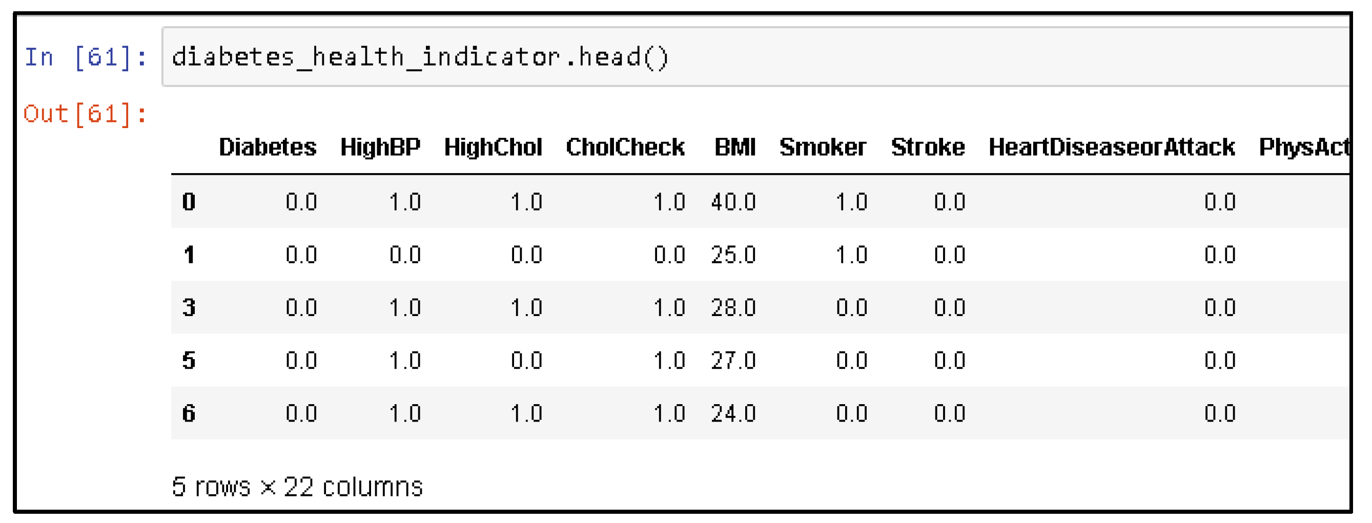
After the data formatting process for each attribute, the attribute name is changed with the rename(columns) function which aims to make it easier to read each attribute in the way shown in Figure 1.

Output result of dataset diabetes_health_indicator:

Figure 2. Output result for upper part of diabetes health indicator dataset.

4.4. Oversampling Data Using SMOTE Technique

The process that is carried out before oversampling is to ensure that the data that is owned is not similar to the other data. Using the duplicate() function, there are 23960 rows that have similarities between rows. Data that has similarities is done by dropping duplicates() so that it produces duplicate data to 0. Separation of data for the independent variable and the dependent variable with ‘y’ as the dependent variable, namely the attribute of Diabetes and ‘x’ as the independent variable, namely the attribute other than Diabetes.

The diabetes attribute has class data that is not balanced with the number of those with diabetes totaling 39657 data and those who are not affected by diabetes totaling 190055 data shown in Figure 3. The results of oversampling on the diabetes attribute with the SMOTE technique using the library imblearn.over_sampling class data that is not balanced with the number those with diabetes have an increase of 65.47% in the class of data affected by diabetes totaling 190055 data and those not affected by diabetes still amounting to 190055 data, shown in Figure 4.

4.5. Feature Selection Algoritma PSO

In the feature selection process using the PSO algorithm, it is done by determining several parameters. Parameter determination is based on research that has been conducted by [23] the parameter includes the constant velocity (

C_{1}, C_{2}

) with the value of 1.49, inertia weight (w) with the value of 0.72, amount of iteration or repeating (N) as much as 100 times and amount of parameter for particles as much as 30. After 100 iterations, the attributes generated by the PSO algorithm will be obtained with a threshold value used to select the best feature with a score above 0.5.

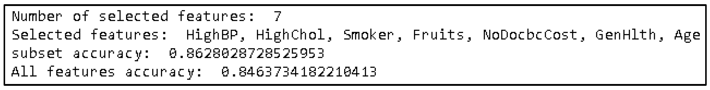
The PSO process in python using the niapy, sys and sklearn libraries shows the results of the selected attributes as many as 7 attributes, namely the attribute HighBP, HighChol, Smoker, Fruits, NoDocbcCost, GenHlth and Age.

Figure 5. The selected attribute results from the PSO algorithm.

The selected attributes have a correlation value between the attributes shown in Figure 6.

The correlation value between the dependent attribute, namely diabetes, and the attribute selected by the PSO algorithm is shown in Table 5.

4.6. Data Mining Result

At the data mining stage, there are two mining processes. First, the classification process with the CART Model Decision Tree algorithm on the Diabetes Health Indicators Dataset. Second, the classification process uses the CART Decision Tree algorithm on the Diabetes Health Indicators Dataset with data oversampling using the SMOTE technique and feature selection using the PSO algorithm.

Data mining with the CART model decision tree algorithm uses the skleran library with import DecisionTreeClassifer and input category 'gini' for classification using the gini index. To evaluate the model using the sklearn.model_selection library with import cross_val_score, KFold and train_test_split. To evaluate the model based on the matrix from the results of the model evaluation using the sklearn.metrics library with import confusion_matrix and classification_report.

The dataset is divided into two, namely training data and test data with a ratio of 80:20. Then, the training data is processed using the CART algorithm and performed k-fold 10 for model testing. In this study, 3 experiments were carried out and then the performance evaluation of the CART algorithm was calculated using the confusion matrix and the MAE value, from the 3 trials, one of the best average accuracy values and the smallest MAE value would be taken.

a.: CART Classification Result

The result of the first classification is the application of the CART Model Decision Tree algorithm classification. Diabetes Health Indicators Dataset is classified using the CART Algorithm without using data oversampling and feature selection. The number of attributes used is 21 attributes and 1 target.

The results of the first CART algorithm trial

Table 6. The results of each fold for accurary, precision, recall, f1-score, APER and MAE values in the first attempt of CART classification.

K-fold	Accurary (%)	Precission (%)	Recall (%)	F1-Score (%)	APER (%)	MAE
1	75,54	31,39	34,12	32,69	24,46	0.2446
2	75,61	30,55	33,39	31,91	24,39	0.2439
3	75,43	30,31	33,70	31,91	24,57	0.2457
4	75,24	30,70	33,51	32,04	24,76	0.2476
5	75,10	30,72	34,01	32,28	24,90	0.2490
6	75,48	30,68	33,53	32,04	24,52	0.2452
7	74,70	30,78	33,72	32,19	25,30	0.2530
8	75,35	31,37	35,71	33,40	24,65	0.2465
9	75,34	29,32	32,31	30,74	24,66	0.2466
10	75,40	29,75	33,79	31,64	24,60	0.2460
Median	75,32	30,56	33,78	32,08	24,68	0.2468

2.: The results of the second CART algorithms trial

Table 7. The results of each fold for accurary, precision, recall, f1-score, APER and MAE values in the second trial of CART classification.

K-fold	Accurary (%)	Precission (%)	Recall (%)	F1-Score (%)	APER (%)	MAE
1	75,58	31,54	34,34	32,88	24,42	0.2442
2	75,82	30,95	33,52	32,18	24,18	0.2418
3	75,32	30,04	33,42	31,64	24,68	0.2468
4	75,35	30,83	33,38	32,06	24,65	0.2465
5	75,26	31,10	34,38	32,66	24,74	0.2474
6	75,21	30,00	32,82	31,34	24,79	0.2479
7	74,71	30,70	33,46	32,02	25,29	0.2529
8	75,33	31,15	35,11	33,01	24,67	0.2467
9	75,38	29,60	32,90	31,16	24,62	0.2462
10	75,60	30,13	33,97	31,94	24,40	0.2440
Median	75,34	30,58	33,75	32,09	24,66	0.2466

3.: The results of the third CART algorithm trial.

Table 8. The results of each fold for accurary, precision, recall, f1-score, APER and MAE values in the three CART classification trials.

K-fold	Accurary (%)	Precission (%)	Recall (%)	F1-Score (%)	APER (%)	MAE
1	75,41	31,10	33,87	32,42	24,59	0.2459
2	75,58	30,73	34,00	32,28	24,42	0.2442
3	75,33	30,14	33,67	31,81	24,67	0.2467
4	75,22	30,49	33,01	31,70	24,78	0.2478
5	75,02	30,64	34,16	32,30	24,98	0.2498
6	75,50	30,81	33,78	32,23	24,50	0.2450
7	74,77	30,88	33,70	32,23	25,23	0.2523
8	75,63	31,83	35,76	33,68	24,37	0.2437
9	75,27	29,34	32,64	30,90	24,73	0.2473
10	75,40	29,82	34,00	31,77	24,60	0.2460
Median	75,33	30,58	33,79	32,10	24,67	0.2467

The results of the CART algorithm experiment using 3 trials resulted in the best trial in the 2nd trial which is shown in Table 9.

The results of the second experiment showed that the highest accuracy of applying the CART algorithm without using data oversampling and feature selection obtained an average accuracy of 75.34%, precision of 30.58%, recall of 33.75%, f1-score of 32, 09%, APER of 24.66% and an MAE value of 0.2466.

b.: SMOTE+PSO+CART Classification Results

The result of the second classification is the application of the CART Model Decision Tree algorithm classification. Diabetes Health Indicators Dataset is classified using the CART + SMOTE + PSO Algorithm The number of attributes used is 7 attributes and 1 target.

The results of the first CART+SMOTE+PSO algorithms.

Table 10. The results of each fold for accurary, precision, recall, f1-score, APER and MAE values in the first attempt of CART + SMOTE + PSO classification.

K-fold	Accurary (%)	Precission (%)	Recall (%)	F1-Score (%)	APER (%)	MAE
1	86,09	92,33	78,73	84,99	13,91	0.1391
2	86,10	92,17	78,91	85,03	13,90	0.1390
3	86,37	93,14	78,74	85,34	13,63	0.1363
4	86,31	92,50	78,94	85,18	13,69	0.1369
5	86,09	91,98	79,00	85,00	13,91	0.1391
6	86,32	92,74	78,93	85,28	13,68	0.1368
7	86,26	92,66	78,88	85,22	13,74	0.1374
8	86,50	92,99	78,99	85,42	13,50	0.1350
9	86,17	92,75	78,52	85,05	13,83	0.1383
10	86,59	92,17	79,56	85,40	13,40	0.1341
Median	86,28	92,54	78,92	85,19	13,72	0.1372

2.: The results of the second CART+SMOTE+PSO algorithms.

Table 11. The results of each fold for accurary, precision, recall, f1-score, APER and MAE values in the second experiment of CART + SMOTE + PSO classification.

K-fold	Accurary (%)	Precission (%)	Recall (%)	F1-Score (%)	APER (%)	MAE
1	86,09	92,33	78,73	84,99	13,91	0.1391
2	86,10	92,17	78,91	85,03	13,90	0.1390
3	86,37	93,14	78,74	85,34	13,63	0.1363
4	86,31	92,50	78,94	85,18	13,69	0.1369
5	86,09	91,98	79,00	85,00	13,91	0.1391
6	86,32	92,74	78,93	85,28	13,68	0.1368
7	86,26	92,66	78,88	85,22	13,73	0.1373
8	86,50	92,99	78,99	85,42	13,50	0.1350
9	86,17	92,75	78,52	85,05	13,83	0.1383
10	86,59	92,17	79,56	85,40	13,41	0.1341
Median	86,28	92,54	78,92	85,19	13,72	0.1372

3.: The results of the third CART+SMOTE+PSO algorithms.

Table 12. The results of each fold for accurary, precision, recall, f1-score, APER and MAE values in the second experiment of CART + SMOTE + PSO classification.

K-fold	Accurary (%)	Precission (%)	Recall (%)	F1-Score (%)	APER (%)	MAE
1	86,09	92,33	78,73	84,99	13,91	0.1391
2	86,10	92,17	78,91	85,03	13,90	0.1390
3	86,37	93,14	78,74	85,34	13,63	0.1363
4	86,31	92,50	78,94	85,18	13,69	0.1369
5	86,09	91,98	79,00	85,00	13,91	0.1391
6	86,32	92,74	78,93	85,28	13,68	0.1368
7	86,26	92,66	78,88	85,22	13,73	0.1373
8	86,50	92,99	78,99	85,42	13,50	0.1350
9	86,17	92,75	78,52	85,05	13,83	0.1383
10	86,59	92,17	79,56	85,40	13,41	0.1341
Median	86,28	92,54	78,92	85,19	13,72	0.1372

The results of the CART algorithm experiment using 3 trials produced the same results from the accurary, precision, recall, f1-score, APER and MAE values shown in Table 13.

The results of the classification experiment show that the highest accuracy of applying the CART algorithm using data oversampling with the SMOTE technique and feature selection with the PSO technique obtains an average accuracy of 86.28%, precision of 92.54%, recall of 78.92%, f1 -score of 85.19%, APER of 13.72% and value MAE 0,1372.

Based on the results above, explained as follows.

1.: Oversampling Data with SMOTE technique for Diabetes Health Indicators Dataset

On the diabetes attribute, the number of people affected by diabetes is 39,657 data and 190055 data were not affected by diabetes after oversampling the data using the SMOTE technique which results in class balanced data between the number of those affected by diabetes 190055 data and 190055 data that are not affected by diabetes have an increase of 65.47% in the data class affected by diabetes.

2.: Feature Selection on the Diabetes Health Indicators Dataset attribute using the PSO algorithm

The application of the PSO algorithm for feature selection uses parameters including speed constants (

C_{1}, C_{2}

) with a value of 1.49, inertial weight (w) with a value of 0.72, the number of iterations or repetitions (N) is 100 times and the number of parameters for particles is 30 particles, the best feature with a score above 0.5 will be selected by the PSO algorithm. The results of the feature selection attribute were selected as many as 7 attributes, namely the attributes HighBP, HighChol, Smoker, Fruits, NoDocbcCost, GenHlth and Age.

3.: Accuracy of the CART model Decision Tree algorithm using SMOTE and PSO

By using data oversampling using the SMOTE technique and feature selection with the PSO algorithm to obtain the best accuracy in the CART model decision tree algorithm. Diabetes Health Indicators Dataset has 380110 rows with 7 attributes and 1 target obtaining an average accuracy of 86.28%, precision of 92.54%, recall of 78.92%, f1-score of 85.19%, APER of 13 .72% and the MAE value is 0.1372. Comparison of the accuracy results performed with the CART model decision tree algorithm using and without oversampling and feature selection can be seen in Table 14.

Conclusions

The conclusions from this study is the increasing accuracy of the classification and regression tree (CART) model for predicting diabetes using the synthetic minority over-sampling technique (SMOTE) and particle swarm optimization (PSO) showed an increase in accuracy of 13.72%, namely 86.28% and has a precision value of 92.54%, recall of 78.92%, f1-score of 85.19%, APER of 13.72% and an MAE value of 0.1372. Suggestions of this study can be developed and compared with other classification algorithms such as C4.5, KNN, Naïve Bayes, Random Forest and SVM and also add boosting algorithms to improve the performance of the classification model so that it becomes a strong learner. The boosting algorithms include AdaBoost, XGBosst and Gradient Boosting.

Author Contributions

Conceptualization, Y.L.S. and M.Z.R.; methodology, Y.L.S. and M.Z.R.; software, M.Z.R.; validation, Y.L.S., and M.Z.R.; data curation, Y.L.S.; original draft, Y.L.S.; review writing and editing, Y.L.S., and M.Z.R.; project administration, M.Z.R.; funding acquisitions, Y.L.S. All authors have read and agree to the published version of the manuscript.

Funding

This research was not funded.

Institutional Review Board Statement

This research was conducted in accordance with the guidelines of the Declaration of Helsinki, and was approved by the Ethics Committee of Semarang State University.

Informed Consent Statement

Informed consent was obtained from all subjects involved in this study.

Data Availability Statement

Data is available by the author without undue reservation.

Conflicts of Interest

The authors declare no conflict of interest.

References

IDF, IDF Diabetes Atlas 2021 – 10th edition, 10th ed., vol. 10. 2021. [CrossRef]
W. C. Hsu, M. R. G. Araneta, A. M. Kanaya, J. L. Chiang, and W. Fujimoto, “BMI cut points to identify at-Risk asian americans for type 2 diabetes screening,” Diabetes Care, vol. 38, no. 1, pp. 150–158, 2015. [CrossRef]
Asidik, Kusrini, and Henderi, “Decision Support System Model of Teacher Recruitment Using Algorithm C4 . 5 and Fuzzy Tahani Decision Support System Model of Teacher Recruitment Using Algorithm C4 . 5 and Fuzzy Tahani,” J. Phys. Conf. Ser. Pap., 2018. [CrossRef]
I. H. Witten, E. Frank, and M. A. Hall, Data Mining Practical Machine Learning Tools and Techniques, 3rd ed. United atates, 2011. [CrossRef]
P. Shella, “Sistem Pendukung Keputusan Dengan Menggunakan Decission Tree Dalam Pemberian Beasiswa Di Sekolah Menengah Pertama (Studi Kasus di SMPN 2 Rembang),” Universitas Negeri Semarang, 2015.
T. Setiyorini and R. T. Asmono, “Komparasi Metode Decision Tree, Naive Bayes Dan K-Nearest Neighbor Pada Klasifikasi Kinerja Siswa,” J. Techno Nusa Mandiri, vol. 15, no. 2, pp. 85–92, 2018. [CrossRef]
J. Han and M. Kamber, Data Mining: Concepts and Techniques : Concepts and Techniques. San Frasisco, 2012.
B. Xue, M. Zhang, and W. N. Browne, “Particle swarm optimisation for feature selection in classification: Novel initialisation and updating mechanisms,” Appl. Soft Comput. J., vol. 18, pp. 261–276, 2014. [CrossRef]
A. Puri and M. K. Gupta, “Comparative Analysis of Resampling Techniques under Noisy Imbalanced Datasets,” IEEE Int. Conf. Issues Challenges Intell. Comput. Tech. ICICT 2019, 2019. [CrossRef]
N. V Chawla, K. W. Bowyer, L. O. Hall, and W. P. Kegelmeyer, “SMOTE: Synthetic Minority Over-sampling Technique,” J. Artif. Intell. Res., vol. 16, no. 2, pp. 321–357, 2002. [CrossRef]
B. Krawczyk, “Learning from imbalanced data: open challenges and future directions,” Prog. Artif. Intell., vol. 5, no. 4, pp. 221–232, 2016. [CrossRef]
A. N. Noercholis, “Comparative Analysis of 5 Algorithm Based Particle Swarm Optimization (Pso) for Prediction of Graduate Time Graduation,” Matics, vol. 12, no. 1, p. 1, 2020. [CrossRef]
K. Ramandana and I. Carolina, “Seleksi Fitur Algoritma Neural Network Menggunakan Particle Swarm Optimization Untuk Memprediksi Kelahiran Prematur,” Kilat, vol. 6, no. 2, pp. 106–111, 2017. [CrossRef]
V. F. Rodriguez-Galiano, J. A. Luque-Espinar, M. Chica-Olmo, and M. P. Mendes, “Feature selection approaches for predictive modelling of groundwater nitrate pollution: An evaluation of filters, embedded and wrapper methods,” Sci. Total Environ., vol. 624, pp. 661–672, 2018. [CrossRef]
T. Dudkina, I. Meniailov, K. Bazilevych, S. Krivtsov, and A. Tkachenko, “Classification and prediction of diabetes disease using decision tree method,” CEUR Workshop Proc., vol. 2824, pp. 163–172, 2021.
Z. Xie, O. Nikolayeva, J. Luo, and D. Li, “Building risk prediction models for type 2 diabetes using machine learning techniques,” Prev. Chronic Dis., vol. 16, no. 9, pp. 1–9, 2019. [CrossRef]
V. Chang, M. A. Ganatra, K. Hall, L. Golightly, and Q. A. Xu, “An assessment of machine learning models and algorithms for early prediction and diagnosis of diabetes using health indicators,” Healthc. Anal., vol. 2, no. September, p. 100118, 2022. [CrossRef]
N. Maulidah et al., “Seleksi Fitur Klasifikasi Penyakit Diabetes Menggunakan Particle Swarm Optimization (PSO) Pada Algoritma Naive Bayes,” Drh. Khusus Ibuk. Jakarta, vol. 13, no. 2, p. 21231170, 2020, [Online]. Available: http://journal.stekom.ac.id/index.php/elkom■page40.
A. N. Rachman, S. Supratman, and E. N. F. Dewi, “Decision Tree and K-Nearest Neighbor (K-NN) Algorithm Based on Particle Swarm Optimization (PSO) for Diabetes Mellitus Prediction Accuracy Analysis,” CESS (Journal Comput. Eng. Syst. Sci., vol. 7, no. 2, p. 315, 2022. [CrossRef]
I. Muqiit WS and R. Nooraeni, “Penerapan Metode Resampling Dalam Mengatasi Imbalanced Data Pada Determinan Kasus Diare Pada Balita Di Indonesia (Analisis Data Sdki 2017),” J. MSA ( Mat. dan Stat. serta Apl. ), vol. 8, no. 1, p. 19, 2020. [CrossRef]
M. A. Muslim et al., Data Mining algoritma c 4.5 Disertai contoh kasus dan penerapannya dengan program computer. 2019.
A. Subasi, Practical Machine Learning for Data Analysis Using Python. 2020. [CrossRef]
M. Qois Syafi, “Increasing Accuracy of Heart Disease Classification on C4.5 Algorithm Based on Information Gain Ratio and Particle Swarm Optimization Using Adaboost Ensemble,” J. Adv. Inf. Syst. Technol., vol. 4, no. 1, pp. 100–112, 2022, [Online]. Available: https://journal.unnes.ac.id/sju/index.php/jaist.

Figure 1. The process of replacing attribute names with function rename(columns).

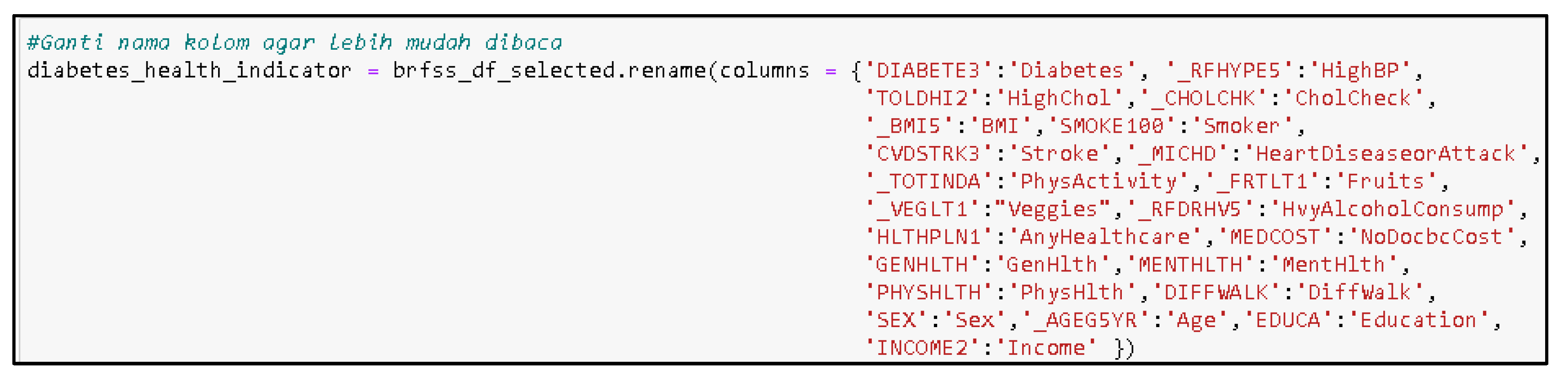
Figure 3. Graph of the number of diabetics who have diabetes (1) and those who do not have diabetes (0).

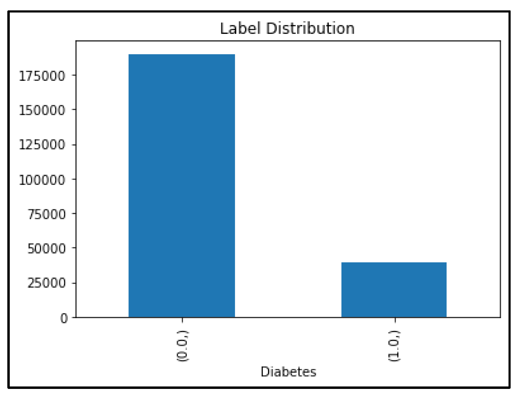
Figure 4. Graph of the number of diabetes classes before oversampling (a) and after oversampling (b).

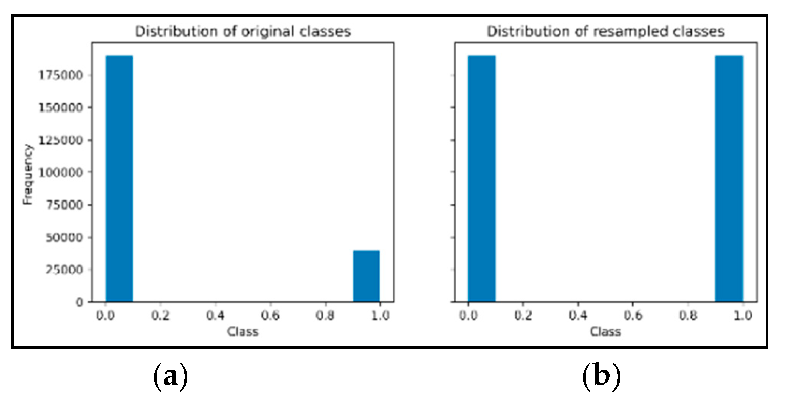
Figure 6. Graph of correlation values between selected attributes.

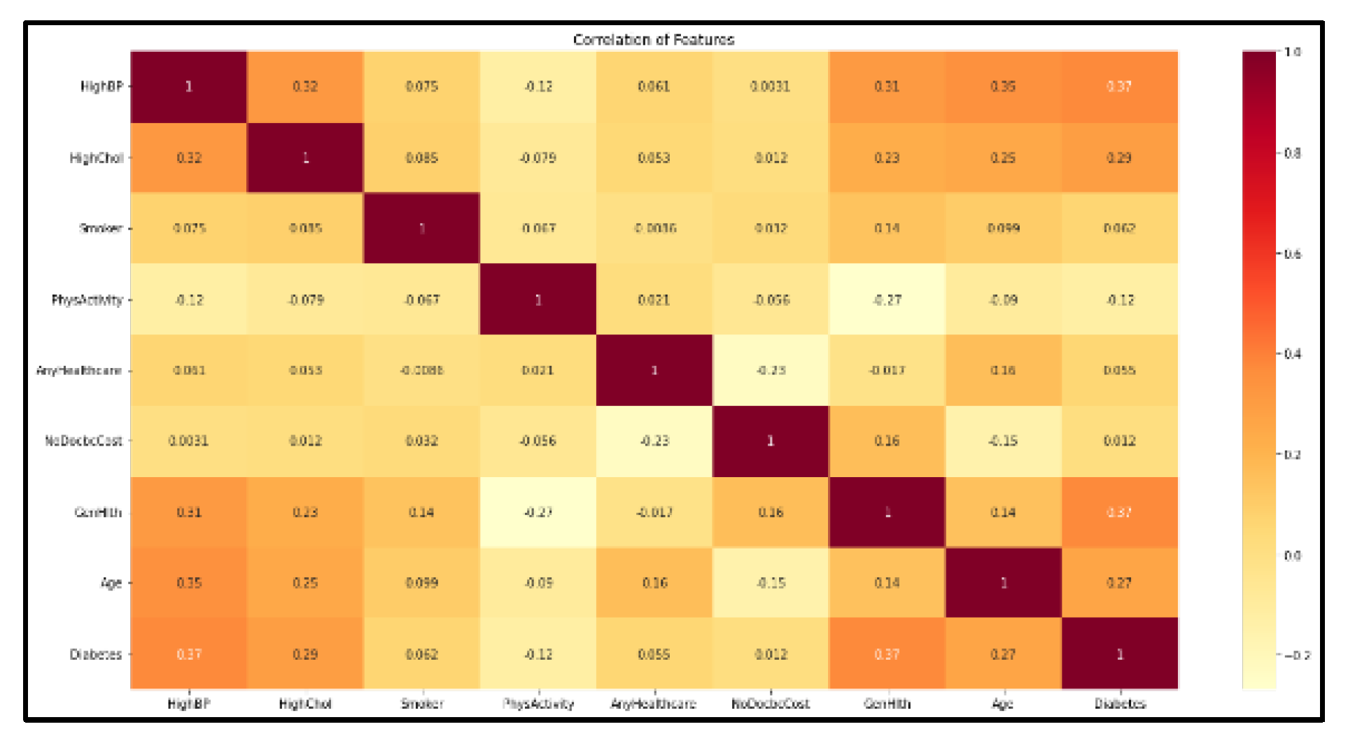
Table 1. Confusion Matrix Table.

Two Class Classification		Actual Class
		0	1
Predicted Class	0	TN		FP
	1	FN		TP

Table 3. Amount of empty data on Diabetes Health Indicators Dataset.

No	Attribute	Empty Data Amount
1	DIABETE3	7
2	TOLDHI2	59154
3	_BMI5	36398
4	SMOKE100	14255
5	“_MICHD	3942
6	DIFFWALK	12334
7	INCOME2	3301

Table 4. Formatting data on Diabetes Health Indicators Dataset.

Variable Name	Formatting
DIABETE3	0 = Have no diabetes symptom 1 = Have diabetes symptoms type 1 or 2
_RFHYPE5	0 = Have no blood pressure 1 = Have blood pressure
TOLDHI2	0 = Have no high cholesterol 1 = Have high cholesterol
c	0 = Have no cholesterol check history within 5 years. 1 = Have cholesterol check history within 5 years.
_BMI5	Integer value BMI
SMOKE100	0 = Does not smoke at least 100 cigarettes before. 1 = Does smoke at least 100 cigarettes before.
_TOTINDA	0 = Have not done any form of workout within 30 days, besides work. 1 = Have done any form of workout within 30 days, besides work.
_FRTLT1	0 = Does not consume at least 1 kind of fruit a day. 1 = Consume at least 1 kind of fruit a day.
_VEGLT1	0 = Does not consume at least 1 kind of vegetable a day. 1 = Consume at least 1 kind of vegetable a day.
_RFDRHV5	0 = Does not consume over 14 liquor for adult male or 7 for female. 1 = Does consume over 14 liquor for adult male or 7 for female.
CVDSTRK3	0 = Have no history of having a stroke. 1 = Have history of having a stroke.
_MICHD	0 = Have no history of having a myocardial infarction (MI). 1 = Have history of having a myocardial infarction (MI).
HLTHPLN1	0 = Does not have health care coverage. 1= Does have health care coverage.
MEDCOST	0 = Does not have a medical chekup within the last 12 months cause of cost. 1 = Does have a medical chekup within the last 12 months.
GENHLTH	0 = Does not state health condition in general. 1 = Excellent 2 = Very good 3 = Good 4 = Pretty good 5 = Bad
MENTHLTH	0 = Have no stress, depretion, and or emotional problem within the last 30 days. 1-30 = Amount of day (s) having stress, depretion, and or emotional problem within the last 30 days.
PHYSHLTH	0 = Have no physical injury within the last 30 days. 1-30 = Amount of days having physical injury within the last 30 days.
DIFFWALK	0 = Have no problem in walking or climbing up stairs. 1 = Have problems in walking or climbing up stairs.
SEX	0 = Female respondent 1 = Male respondent
_AGEG5YR	Respondent age category 1 = 18-24 y.o 2 = 25-29 y.o 3 = 30-34 y.o 4 = 35-39 y.o 5 = 40-44 y.o 6 = 45-49 y.o 7 = 50-54 y.o 8 = 55-59 y.o 9 = 60-64 y.o 10 = 65-69 y.o 11 = 70-74 y.o 12 = 75-79 y.o 13 = 80 y.o or above
EDUCA	Respondent last educational level category 1 = Have not or never kindergarten 2 = Pass between elementary school 3 = Pass between highschool 4 = Pass highschool 5 = Pass between college or technical school 6 = Pass college
INCOME2	Respondent income categories for a year in dollars 1 = Lower than USD 10.000 2 = USD 10.000 – USD 15.000 3 = USD 15.000 – USD 20.000 4 = USD 20.000 – USD 25.000 5 = USD 25.000 – USD 35.000 6 = USD 35.000 – USD 50.000 7 = USD 50.000 – USD 75.000 8 = Over USD 75.000

Table 5. Correlation value between diabetes attributes and selected attributes.

Attribute Name	Correlation Value
HighBP	0.37
HighChol	0.29
Smoker	0.062
Fruits	0.12
NoDocbcCost	0.012
GenHlth	0.37
Age	0.27

Table 9. Mean value results in 3 CART classification trials.

Trial	Accurary (%)	Precission (%)	Recall (%)	F1-Score (%)	APER (%)	MAE
1	75,32	30,56	33,78	32,08	24,68	0.2468
2	75,34	30,58	33,75	32,09	24,66	0.2466
3	75,33	30,58	33,79	32,10	24,67	0.2467

Table 13. Average value results in 3 CART + SMOTE + PSO classification trials.

Trial	Accurary (%)	Precission (%)	Recall (%)	F1-Score (%)	APER (%)	MAE
1	86,28	92,54	78,92	85,19	13,72	0.1372
2	86,28	92,54	78,92	85,19	13,72	0.1372
3	86,28	92,54	78,92	85,19	13,72	0.1372

Table 14. Final Results of Research Accuracy.

Algorithm	Accuracy Result
CART	75,34%
CART + SMOTE + PSO	86,28%

Disclaimer/Publisher’s Note: The statements, opinions and data contained in all publications are solely those of the individual author(s) and contributor(s) and not of MDPI and/or the editor(s). MDPI and/or the editor(s) disclaim responsibility for any injury to people or property resulting from any ideas, methods, instructions or products referred to in the content.

© 2023 by the authors. Licensee MDPI, Basel, Switzerland. This article is an open access article distributed under the terms and conditions of the Creative Commons Attribution (CC BY) license (http://creativecommons.org/licenses/by/4.0/).

Copyright: This open access article is published under a Creative Commons CC BY 4.0 license, which permit the free download, distribution, and reuse, provided that the author and preprint are cited in any reuse.

Submitted:

04 June 2023

Posted:

05 June 2023

You are already at the latest version

Alerts

Abstract

Keywords:

Subject: Computer Science and Mathematics - Applied Mathematics

Introduction

x_{i} = (x_{i 1}, x_{12}, \dots, x_{i D})

x_{i} = (x_{i 1}, x_{12}, \dots, x_{i D})

v_{i} = (v_{i 1}, v_{i 2}, v_{i D})

Method

In this research, several stages of research steps were carried out. Namely: literature study, problem formulation, data and data sources, data analysis and drawing conclusions.

2.1. Literature Review

2.2. Data and Data Source

2.3. Data Analysis

Import Data

Preprocessing

x_{s y n} = x_{i} + {(x_{k n n} - x_{i})}^{} x τ

As:

x_{s y n}

=data from resampling

x_{i}

=data that will be replicated

x_{k n n}

=data with the closes distance from the replicated data.

τ

= random numbering 0-1

Feature Selection

Initialization: done randomly to determine the initial particle.
Fitness: a measure in each particle in the population.
Update: calculate the velocity of each particle with the equation below.

v_{j}^{t + 1} = w . v_{j}^{t} + c_{1} . r_{1} ({p B e s t}_{j}^{t} - x_{j}^{t}) + c_{2} . r_{2} ({g B e s t}_{j}^{t} - x_{j}^{t})

As:

v_{j}^{t + 1}

= particle velocity

j

on iteration

v_{j}^{t}

= particle velocity

j

on iteration to-

t

x_{j}^{t}

= particle position

j

on iteration to-

t

w

= inertial weight

c_{1}, c_{2}

= constant velocity

r_{1}, r_{2}

= random numbering

\in [0,1]

{p B e s t}_{j}^{t}

= best position for particle

j

on iteration to-

t

{g B e s t}_{j}^{t}

= global optimal for particle

j

on iteration to-

t

1): Construction with the equation below.

x_{j}^{t + 1} = x_{j}^{t} + v_{j}^{t + 1}

2): Termination: stop the process, if the termination criteria are met, and return to step 2 (fitness) if not met.

Split Data

On the data splitting process, the dataset is divided into two parts. Namely, test data and training data with a ratio of 80:20, 80% as training data and 20% as test data.

Algorithm clarification method on decision tree model Classification and Regression Trees (CART)

On the CART classification process with stages:

1): Determination of the variables to be tested.
2): Determining the number of sorters per variable according to the type of independent variable using the equation below.

b - 1 s e l e c t i o n

: Continues independent variable

2^{L - 1} - 1 s e l e c t i o n

: Nominal category independent variable

L - 1 p e m i l a h a n

: Ordinal category independent variable

As:

b

= Amount of data on a variable

L

= Amount of category on a variable

3): Calculate the ‘Gini index’ value for each sorter according to the equation below.

i (t) = 1 - \sum_{j = 1} P^{2} (j | t)

As:

i (t)

= Gini index

P (j| t)

= Class proportion j on node t

n_{j} (t)

= Amount of observation on class j node t

n (t)

= Amount of observation on node t

Then the sorter that has the smallest Gini index value will be chosen to be the best sorter.

4): Repeat step 2-3 to perform sorting until it is no longer possible.
5): Marking of terminal node class labels is based on the rules for the highest number of members using the equation below.

P (j| t) = {m a x}_{j} \frac{N_{j} (t)}{N (t)}

As:

P (j| t)

= Probability of class j on node t

N_{j} (t)

= Amount of observation on class j node t

N (t)

= Amount of observation on node t

Testing and Algorithm Evaluation

1): Insert testing result on the confusion matrix Table 1.

As:

TN : True Negatif

FP : False Positive

FN : False Negatif

TP : True Positive

2): Calculate the accuracy value using the equation.

a c c u r a r y = \frac{T P + T N}{T P + F P + T N + F N}

The level of precission using the equation.

p r e c i s s i o n = \frac{T P}{T P + F P}

Recall value using the equation.

r e c a l l = \frac{T P}{T P + F N}

The value of the F1 score uses the equation.

F 1 s c o r e = \frac{2 \times p r e c i s s i o n \times r e c a l l}{p r e c i s s i o n + r e c a l l}

APER value uses the equation.

A P E R = \frac{F P + F N}{T P + F P + T N + F N} x 100 %

MAE (Mean Absolute Error) value is used to calculate the average difference between the calculated value and the actual value [22] uses the equation.

M A E = \frac{\sum_{{u, i}} |p_{u i} - r_{u i}|}{N}

As:

p_{u i}

= prediction value.

r_{u i}

= actual value.

N = amount of data lines.

Result and Discussion

4.1. Data Mining

Data mined and used in this research is "Diabetes Health Indicators Dataset" from Kaggle in the form of Comma Separated Values (CSV). The attributes used are 22 attributes namely.

Table 2. Data attribute on Diabetes Health Indicators Dataset.

No	Attribute	Variable Name
1	Diabetes Disease	DIABETE3
2	High Blood Pressure	_RFHYPE5
3	High Cholesterol	TOLDHI2
4	Cholesterol Check	_CHOLCHK
5	BMI (Body Mass Index)	_BMI5
6	Smoker	SMOKE100
7	Physical Activity	_TOTINDA
8	Consume Fruit	_FRTLT1
9	Consume Vegetables	_VEGLT1
10	Alcohol Consumption	_RFDRHV5
11	Stroke	CVDSTRK3
12	Heart Disease	_MICHD
13	Health Care Coverage	HLTHPLN1
14	Medical Checkup	MEDCOST
15	General Health	GENHLTH
16	Mental Health	MENTHLTH
17	Physical Health	PHYSHLTH
18	Difficult Walking Or Climbing Stairs	DIFFWALK
19	Sex	SEX
20	Age Category	_AGEG5YR
21	Highest Grade School	EDUCA
22	Income	INCOME2

4.2. Data Cleaning

After that, the drop missing value was carried out using the dropna() function to produce 343,406 new data rows and 22 attributes.

4.3. Formatting Data

The data formatting stage aims to standardize the format of the dataset used in the research. The formatting performed on the Diabetes Health Indicators Dataset is shown in Table 4.

After the data formatting process for each attribute, the attribute name is changed with the rename(columns) function which aims to make it easier to read each attribute in the way shown in Figure 1.

Output result of dataset diabetes_health_indicator:

Figure 2. Output result for upper part of diabetes health indicator dataset.

4.4. Oversampling Data Using SMOTE Technique

4.5. Feature Selection Algoritma PSO

C_{1}, C_{2}

Figure 5. The selected attribute results from the PSO algorithm.

The selected attributes have a correlation value between the attributes shown in Figure 6.

The correlation value between the dependent attribute, namely diabetes, and the attribute selected by the PSO algorithm is shown in Table 5.

4.6. Data Mining Result

a.: CART Classification Result

The results of the first CART algorithm trial

Table 6. The results of each fold for accurary, precision, recall, f1-score, APER and MAE values in the first attempt of CART classification.

K-fold	Accurary (%)	Precission (%)	Recall (%)	F1-Score (%)	APER (%)	MAE
1	75,54	31,39	34,12	32,69	24,46	0.2446
2	75,61	30,55	33,39	31,91	24,39	0.2439
3	75,43	30,31	33,70	31,91	24,57	0.2457
4	75,24	30,70	33,51	32,04	24,76	0.2476
5	75,10	30,72	34,01	32,28	24,90	0.2490
6	75,48	30,68	33,53	32,04	24,52	0.2452
7	74,70	30,78	33,72	32,19	25,30	0.2530
8	75,35	31,37	35,71	33,40	24,65	0.2465
9	75,34	29,32	32,31	30,74	24,66	0.2466
10	75,40	29,75	33,79	31,64	24,60	0.2460
Median	75,32	30,56	33,78	32,08	24,68	0.2468

2.: The results of the second CART algorithms trial

Table 7. The results of each fold for accurary, precision, recall, f1-score, APER and MAE values in the second trial of CART classification.

K-fold	Accurary (%)	Precission (%)	Recall (%)	F1-Score (%)	APER (%)	MAE
1	75,58	31,54	34,34	32,88	24,42	0.2442
2	75,82	30,95	33,52	32,18	24,18	0.2418
3	75,32	30,04	33,42	31,64	24,68	0.2468
4	75,35	30,83	33,38	32,06	24,65	0.2465
5	75,26	31,10	34,38	32,66	24,74	0.2474
6	75,21	30,00	32,82	31,34	24,79	0.2479
7	74,71	30,70	33,46	32,02	25,29	0.2529
8	75,33	31,15	35,11	33,01	24,67	0.2467
9	75,38	29,60	32,90	31,16	24,62	0.2462
10	75,60	30,13	33,97	31,94	24,40	0.2440
Median	75,34	30,58	33,75	32,09	24,66	0.2466

3.: The results of the third CART algorithm trial.

Table 8. The results of each fold for accurary, precision, recall, f1-score, APER and MAE values in the three CART classification trials.

K-fold	Accurary (%)	Precission (%)	Recall (%)	F1-Score (%)	APER (%)	MAE
1	75,41	31,10	33,87	32,42	24,59	0.2459
2	75,58	30,73	34,00	32,28	24,42	0.2442
3	75,33	30,14	33,67	31,81	24,67	0.2467
4	75,22	30,49	33,01	31,70	24,78	0.2478
5	75,02	30,64	34,16	32,30	24,98	0.2498
6	75,50	30,81	33,78	32,23	24,50	0.2450
7	74,77	30,88	33,70	32,23	25,23	0.2523
8	75,63	31,83	35,76	33,68	24,37	0.2437
9	75,27	29,34	32,64	30,90	24,73	0.2473
10	75,40	29,82	34,00	31,77	24,60	0.2460
Median	75,33	30,58	33,79	32,10	24,67	0.2467

The results of the CART algorithm experiment using 3 trials resulted in the best trial in the 2nd trial which is shown in Table 9.

b.: SMOTE+PSO+CART Classification Results

The results of the first CART+SMOTE+PSO algorithms.

Table 10. The results of each fold for accurary, precision, recall, f1-score, APER and MAE values in the first attempt of CART + SMOTE + PSO classification.

K-fold	Accurary (%)	Precission (%)	Recall (%)	F1-Score (%)	APER (%)	MAE
1	86,09	92,33	78,73	84,99	13,91	0.1391
2	86,10	92,17	78,91	85,03	13,90	0.1390
3	86,37	93,14	78,74	85,34	13,63	0.1363
4	86,31	92,50	78,94	85,18	13,69	0.1369
5	86,09	91,98	79,00	85,00	13,91	0.1391
6	86,32	92,74	78,93	85,28	13,68	0.1368
7	86,26	92,66	78,88	85,22	13,74	0.1374
8	86,50	92,99	78,99	85,42	13,50	0.1350
9	86,17	92,75	78,52	85,05	13,83	0.1383
10	86,59	92,17	79,56	85,40	13,40	0.1341
Median	86,28	92,54	78,92	85,19	13,72	0.1372

2.: The results of the second CART+SMOTE+PSO algorithms.

Table 11. The results of each fold for accurary, precision, recall, f1-score, APER and MAE values in the second experiment of CART + SMOTE + PSO classification.

K-fold	Accurary (%)	Precission (%)	Recall (%)	F1-Score (%)	APER (%)	MAE
1	86,09	92,33	78,73	84,99	13,91	0.1391
2	86,10	92,17	78,91	85,03	13,90	0.1390
3	86,37	93,14	78,74	85,34	13,63	0.1363
4	86,31	92,50	78,94	85,18	13,69	0.1369
5	86,09	91,98	79,00	85,00	13,91	0.1391
6	86,32	92,74	78,93	85,28	13,68	0.1368
7	86,26	92,66	78,88	85,22	13,73	0.1373
8	86,50	92,99	78,99	85,42	13,50	0.1350
9	86,17	92,75	78,52	85,05	13,83	0.1383
10	86,59	92,17	79,56	85,40	13,41	0.1341
Median	86,28	92,54	78,92	85,19	13,72	0.1372

3.: The results of the third CART+SMOTE+PSO algorithms.

Table 12. The results of each fold for accurary, precision, recall, f1-score, APER and MAE values in the second experiment of CART + SMOTE + PSO classification.

K-fold	Accurary (%)	Precission (%)	Recall (%)	F1-Score (%)	APER (%)	MAE
1	86,09	92,33	78,73	84,99	13,91	0.1391
2	86,10	92,17	78,91	85,03	13,90	0.1390
3	86,37	93,14	78,74	85,34	13,63	0.1363
4	86,31	92,50	78,94	85,18	13,69	0.1369
5	86,09	91,98	79,00	85,00	13,91	0.1391
6	86,32	92,74	78,93	85,28	13,68	0.1368
7	86,26	92,66	78,88	85,22	13,73	0.1373
8	86,50	92,99	78,99	85,42	13,50	0.1350
9	86,17	92,75	78,52	85,05	13,83	0.1383
10	86,59	92,17	79,56	85,40	13,41	0.1341
Median	86,28	92,54	78,92	85,19	13,72	0.1372

The results of the CART algorithm experiment using 3 trials produced the same results from the accurary, precision, recall, f1-score, APER and MAE values shown in Table 13.

Based on the results above, explained as follows.

1.: Oversampling Data with SMOTE technique for Diabetes Health Indicators Dataset

2.: Feature Selection on the Diabetes Health Indicators Dataset attribute using the PSO algorithm

The application of the PSO algorithm for feature selection uses parameters including speed constants (

C_{1}, C_{2}

3.: Accuracy of the CART model Decision Tree algorithm using SMOTE and PSO

Conclusions

Author Contributions

Funding

This research was not funded.

Institutional Review Board Statement

This research was conducted in accordance with the guidelines of the Declaration of Helsinki, and was approved by the Ethics Committee of Semarang State University.

Informed Consent Statement

Informed consent was obtained from all subjects involved in this study.

Data Availability Statement

Data is available by the author without undue reservation.

Conflicts of Interest

The authors declare no conflict of interest.

References

IDF, IDF Diabetes Atlas 2021 – 10th edition, 10th ed., vol. 10. 2021. [CrossRef]
W. C. Hsu, M. R. G. Araneta, A. M. Kanaya, J. L. Chiang, and W. Fujimoto, “BMI cut points to identify at-Risk asian americans for type 2 diabetes screening,” Diabetes Care, vol. 38, no. 1, pp. 150–158, 2015. [CrossRef]
Asidik, Kusrini, and Henderi, “Decision Support System Model of Teacher Recruitment Using Algorithm C4 . 5 and Fuzzy Tahani Decision Support System Model of Teacher Recruitment Using Algorithm C4 . 5 and Fuzzy Tahani,” J. Phys. Conf. Ser. Pap., 2018. [CrossRef]
I. H. Witten, E. Frank, and M. A. Hall, Data Mining Practical Machine Learning Tools and Techniques, 3rd ed. United atates, 2011. [CrossRef]
P. Shella, “Sistem Pendukung Keputusan Dengan Menggunakan Decission Tree Dalam Pemberian Beasiswa Di Sekolah Menengah Pertama (Studi Kasus di SMPN 2 Rembang),” Universitas Negeri Semarang, 2015.
T. Setiyorini and R. T. Asmono, “Komparasi Metode Decision Tree, Naive Bayes Dan K-Nearest Neighbor Pada Klasifikasi Kinerja Siswa,” J. Techno Nusa Mandiri, vol. 15, no. 2, pp. 85–92, 2018. [CrossRef]
J. Han and M. Kamber, Data Mining: Concepts and Techniques : Concepts and Techniques. San Frasisco, 2012.
B. Xue, M. Zhang, and W. N. Browne, “Particle swarm optimisation for feature selection in classification: Novel initialisation and updating mechanisms,” Appl. Soft Comput. J., vol. 18, pp. 261–276, 2014. [CrossRef]
A. Puri and M. K. Gupta, “Comparative Analysis of Resampling Techniques under Noisy Imbalanced Datasets,” IEEE Int. Conf. Issues Challenges Intell. Comput. Tech. ICICT 2019, 2019. [CrossRef]
N. V Chawla, K. W. Bowyer, L. O. Hall, and W. P. Kegelmeyer, “SMOTE: Synthetic Minority Over-sampling Technique,” J. Artif. Intell. Res., vol. 16, no. 2, pp. 321–357, 2002. [CrossRef]
B. Krawczyk, “Learning from imbalanced data: open challenges and future directions,” Prog. Artif. Intell., vol. 5, no. 4, pp. 221–232, 2016. [CrossRef]
A. N. Noercholis, “Comparative Analysis of 5 Algorithm Based Particle Swarm Optimization (Pso) for Prediction of Graduate Time Graduation,” Matics, vol. 12, no. 1, p. 1, 2020. [CrossRef]
K. Ramandana and I. Carolina, “Seleksi Fitur Algoritma Neural Network Menggunakan Particle Swarm Optimization Untuk Memprediksi Kelahiran Prematur,” Kilat, vol. 6, no. 2, pp. 106–111, 2017. [CrossRef]
V. F. Rodriguez-Galiano, J. A. Luque-Espinar, M. Chica-Olmo, and M. P. Mendes, “Feature selection approaches for predictive modelling of groundwater nitrate pollution: An evaluation of filters, embedded and wrapper methods,” Sci. Total Environ., vol. 624, pp. 661–672, 2018. [CrossRef]
T. Dudkina, I. Meniailov, K. Bazilevych, S. Krivtsov, and A. Tkachenko, “Classification and prediction of diabetes disease using decision tree method,” CEUR Workshop Proc., vol. 2824, pp. 163–172, 2021.
Z. Xie, O. Nikolayeva, J. Luo, and D. Li, “Building risk prediction models for type 2 diabetes using machine learning techniques,” Prev. Chronic Dis., vol. 16, no. 9, pp. 1–9, 2019. [CrossRef]
V. Chang, M. A. Ganatra, K. Hall, L. Golightly, and Q. A. Xu, “An assessment of machine learning models and algorithms for early prediction and diagnosis of diabetes using health indicators,” Healthc. Anal., vol. 2, no. September, p. 100118, 2022. [CrossRef]
N. Maulidah et al., “Seleksi Fitur Klasifikasi Penyakit Diabetes Menggunakan Particle Swarm Optimization (PSO) Pada Algoritma Naive Bayes,” Drh. Khusus Ibuk. Jakarta, vol. 13, no. 2, p. 21231170, 2020, [Online]. Available: http://journal.stekom.ac.id/index.php/elkom■page40.
A. N. Rachman, S. Supratman, and E. N. F. Dewi, “Decision Tree and K-Nearest Neighbor (K-NN) Algorithm Based on Particle Swarm Optimization (PSO) for Diabetes Mellitus Prediction Accuracy Analysis,” CESS (Journal Comput. Eng. Syst. Sci., vol. 7, no. 2, p. 315, 2022. [CrossRef]
I. Muqiit WS and R. Nooraeni, “Penerapan Metode Resampling Dalam Mengatasi Imbalanced Data Pada Determinan Kasus Diare Pada Balita Di Indonesia (Analisis Data Sdki 2017),” J. MSA ( Mat. dan Stat. serta Apl. ), vol. 8, no. 1, p. 19, 2020. [CrossRef]
M. A. Muslim et al., Data Mining algoritma c 4.5 Disertai contoh kasus dan penerapannya dengan program computer. 2019.
A. Subasi, Practical Machine Learning for Data Analysis Using Python. 2020. [CrossRef]
M. Qois Syafi, “Increasing Accuracy of Heart Disease Classification on C4.5 Algorithm Based on Information Gain Ratio and Particle Swarm Optimization Using Adaboost Ensemble,” J. Adv. Inf. Syst. Technol., vol. 4, no. 1, pp. 100–112, 2022, [Online]. Available: https://journal.unnes.ac.id/sju/index.php/jaist.

Figure 1. The process of replacing attribute names with function rename(columns).

Figure 3. Graph of the number of diabetics who have diabetes (1) and those who do not have diabetes (0).

Figure 4. Graph of the number of diabetes classes before oversampling (a) and after oversampling (b).

Figure 6. Graph of correlation values between selected attributes.

Table 1. Confusion Matrix Table.

Two Class Classification		Actual Class
		0	1
Predicted Class	0	TN		FP
	1	FN		TP

Table 3. Amount of empty data on Diabetes Health Indicators Dataset.

No	Attribute	Empty Data Amount
1	DIABETE3	7
2	TOLDHI2	59154
3	_BMI5	36398
4	SMOKE100	14255
5	“_MICHD	3942
6	DIFFWALK	12334
7	INCOME2	3301

Table 4. Formatting data on Diabetes Health Indicators Dataset.

Variable Name	Formatting
DIABETE3	0 = Have no diabetes symptom 1 = Have diabetes symptoms type 1 or 2
_RFHYPE5	0 = Have no blood pressure 1 = Have blood pressure
TOLDHI2	0 = Have no high cholesterol 1 = Have high cholesterol
c	0 = Have no cholesterol check history within 5 years. 1 = Have cholesterol check history within 5 years.
_BMI5	Integer value BMI
SMOKE100	0 = Does not smoke at least 100 cigarettes before. 1 = Does smoke at least 100 cigarettes before.
_TOTINDA	0 = Have not done any form of workout within 30 days, besides work. 1 = Have done any form of workout within 30 days, besides work.
_FRTLT1	0 = Does not consume at least 1 kind of fruit a day. 1 = Consume at least 1 kind of fruit a day.
_VEGLT1	0 = Does not consume at least 1 kind of vegetable a day. 1 = Consume at least 1 kind of vegetable a day.
_RFDRHV5	0 = Does not consume over 14 liquor for adult male or 7 for female. 1 = Does consume over 14 liquor for adult male or 7 for female.
CVDSTRK3	0 = Have no history of having a stroke. 1 = Have history of having a stroke.
_MICHD	0 = Have no history of having a myocardial infarction (MI). 1 = Have history of having a myocardial infarction (MI).
HLTHPLN1	0 = Does not have health care coverage. 1= Does have health care coverage.
MEDCOST	0 = Does not have a medical chekup within the last 12 months cause of cost. 1 = Does have a medical chekup within the last 12 months.
GENHLTH	0 = Does not state health condition in general. 1 = Excellent 2 = Very good 3 = Good 4 = Pretty good 5 = Bad
MENTHLTH	0 = Have no stress, depretion, and or emotional problem within the last 30 days. 1-30 = Amount of day (s) having stress, depretion, and or emotional problem within the last 30 days.
PHYSHLTH	0 = Have no physical injury within the last 30 days. 1-30 = Amount of days having physical injury within the last 30 days.
DIFFWALK	0 = Have no problem in walking or climbing up stairs. 1 = Have problems in walking or climbing up stairs.
SEX	0 = Female respondent 1 = Male respondent
_AGEG5YR	Respondent age category 1 = 18-24 y.o 2 = 25-29 y.o 3 = 30-34 y.o 4 = 35-39 y.o 5 = 40-44 y.o 6 = 45-49 y.o 7 = 50-54 y.o 8 = 55-59 y.o 9 = 60-64 y.o 10 = 65-69 y.o 11 = 70-74 y.o 12 = 75-79 y.o 13 = 80 y.o or above
EDUCA	Respondent last educational level category 1 = Have not or never kindergarten 2 = Pass between elementary school 3 = Pass between highschool 4 = Pass highschool 5 = Pass between college or technical school 6 = Pass college
INCOME2	Respondent income categories for a year in dollars 1 = Lower than USD 10.000 2 = USD 10.000 – USD 15.000 3 = USD 15.000 – USD 20.000 4 = USD 20.000 – USD 25.000 5 = USD 25.000 – USD 35.000 6 = USD 35.000 – USD 50.000 7 = USD 50.000 – USD 75.000 8 = Over USD 75.000

Table 5. Correlation value between diabetes attributes and selected attributes.

Attribute Name	Correlation Value
HighBP	0.37
HighChol	0.29
Smoker	0.062
Fruits	0.12
NoDocbcCost	0.012
GenHlth	0.37
Age	0.27

Table 9. Mean value results in 3 CART classification trials.

Trial	Accurary (%)	Precission (%)	Recall (%)	F1-Score (%)	APER (%)	MAE
1	75,32	30,56	33,78	32,08	24,68	0.2468
2	75,34	30,58	33,75	32,09	24,66	0.2466
3	75,33	30,58	33,79	32,10	24,67	0.2467

Table 13. Average value results in 3 CART + SMOTE + PSO classification trials.

Trial	Accurary (%)	Precission (%)	Recall (%)	F1-Score (%)	APER (%)	MAE
1	86,28	92,54	78,92	85,19	13,72	0.1372
2	86,28	92,54	78,92	85,19	13,72	0.1372
3	86,28	92,54	78,92	85,19	13,72	0.1372

Table 14. Final Results of Research Accuracy.

Algorithm	Accuracy Result
CART	75,34%
CART + SMOTE + PSO	86,28%

MDPI Initiatives

Important Links

Choose an area of interest and we will send you notifications of new preprints at your preferred frequency.

Disclaimer

Accuracy Improved Classification and Regression Tree (CART) Model: Diabetes Prediction Using Minority Over-Sampling and Particle Swarm Optimization Techniques

Abstract

Introduction

Method

2.1. Literature Review

2.2. Data and Data Source

2.3. Data Analysis

Result and Discussion

4.1. Data Mining

4.2. Data Cleaning

4.3. Formatting Data

4.4. Oversampling Data Using SMOTE Technique

4.5. Feature Selection Algoritma PSO

4.6. Data Mining Result

Conclusions

Author Contributions

Funding

Institutional Review Board Statement

Informed Consent Statement

Data Availability Statement

Conflicts of Interest

References

Abstract

Introduction

Method

2.1. Literature Review

2.2. Data and Data Source

2.3. Data Analysis

Result and Discussion

4.1. Data Mining

4.2. Data Cleaning

4.3. Formatting Data

4.4. Oversampling Data Using SMOTE Technique

4.5. Feature Selection Algoritma PSO

4.6. Data Mining Result

Conclusions

Author Contributions

Funding

Institutional Review Board Statement

Informed Consent Statement

Data Availability Statement

Conflicts of Interest

References

MDPI Initiatives

Important Links

Subscribe