Robust Multi-Criteria Traffic Network Equilibrium Problems with Path Capacity Constraints

Preprint

Article

Robust Multi-Criteria Traffic Network Equilibrium Problems with Path Capacity Constraints

Altmetrics

Downloads

Views

Comments

A peer-reviewed article of this preprint also exists.

This version is not peer-reviewed

Submitted:

06 June 2023

Posted:

06 June 2023

You are already at the latest version

Alerts

Abstract

This paper focuses on robust multi-criteria traffic network equilibrium problems with path capacity constraints. The concepts of robust vector equilibrium and robust vector equilibrium with respect to worst case are introduced, respectively. To generate a subset of robust vector equilibrium, an equivalent min-max optimization problem is constructed. In addition, a direct search algorithm, in which the step size without derivatives and redundant parameters, for solving this min-max problem is proposed. To find a subset of robust vector equilibrium with respect to worst case, an equivalent smoothing optimization problem based on a variant version of ReLU activation function is established. Numerical experiments are also presented to expound the advantages of the algorithms.

Keywords:

Subject: Computer Science and Mathematics - Mathematics

1. Introduction

The equilibrium problem of traffic network is to describe the distribution of traffic flow in logistics industry and transportation networks, which is expected to provide an effective method to alleviate traffic congestion. The fundamental principle in the model is the concept of equilibrium that was initially introduced by Wardrop [1], which describes the user behavior in traffic networks. In other words, users will choose a path with the minimum travel cost. Now, it has been shown that Wardrop equilibrium concept is a powerful principle which widely used in supply and demand network, traffic assignment, optimization of traffic control and other fields and so on (see, e.g., Athanasenas, [2]; Nagurney, [3]; Ji and Chu, [4]; Xu et al., [5]; Wang et al., [6]; Ma et al., [7]).

It is worth noting that most of these equilibrium models in the above references are based on a single criterion. Travelers (in this paper, we use the user and traveler interchangeably) will naturally consider many criteria when choosing travel paths, including travel time, distance, cost, weather and safety other relevant factors. The equilibrium model ground on multi-criteria is first put forward by Chen and Yen [8], which is an extension of classical Wardrop user optimization principle. Regarding theoretical analysis for multi-criteria traffic equilibrium models, we refer the reader to Yang and Goh [9]; Li et al.[10], Luc et al.[11], Raith and Ehrgott[12] for further contributions. Recently, Phuong and Luc [13] established the equivalent relationship between strong vector equilibrium flows and the solutions of variational inequality problems in terms of a kind of increasing functions. Moreover, they presented a method to handle multi-criteria network equilibrium problems. Subsequently, Luc and Phuong [14] put forward a modified Frank-Wolfe gradient algorithm for multi-criteria network equilibrium problems. After that, Phuong [15] proposed a smoothing method to solve multi-criteria network equilibrium problems. Numerical methods proposed in Phuong and Luc [13], Luc and Phuong [14] and Phuong [15], can be seen as a first step for the computation of multi-criteria network equilibrium problems.

Considering the influence of uncertain factors in traffic network on traveler behavior, data uncertainty in the logistics industry and transportation receives more and more attentions. Recently, some related works with uncertain demands or cost functions with parameters that are in a set, have been investigated in Daniele and Giuffr [16], Ehrgott et al.[17], Wang et al.[6], Cao et al.[18], Minh and Phuong [19] and Wei et al.[20]. However, to the best of our knowledge, only one work [19] pays attention to the computation for robust equilibrium flows with uncertain cost functions. This prompts us to continuously investigate this topic.

In this paper, we give robust vector equilibrium principle and robust vector equilibrium principle with respect to worst case. An equivalent min-max optimization problem is constructed, in which the solution is equivalent to the robust vector equilibrium flow. A direct search algorithm with constraints for solving this problem is proposed. For robust vector equilibrium with respect to worst case, we transform it into an equilibrium optimization problem based on a variant version of ReLU activation function.

In summary, the contributions of the manuscript are gathered as follows:

(1) Robust vector equilibrium and robust vector equilibrium with respect to worst case principles are introduced.

(2) An equivalent min-max optimization problem is established and then a direct search algorithm is proposed to generate a subset of robust vector equilibrium flows.

(3) To generate a subset of robust vector equilibrium with respect to worst case, a two-step strategy is implemented. Specifically, construct a smoothing optimization problem based on a variant version of ReLU activation function to compute robust weak vector equilibrium flows with respect to worst case and then find robust vector equilibrium flows with respect to worst case by using Heaviside Step function.

This paper is divided into the following parts. Section 2 mainly introduces robust vector equilibrium principle and robust vector equilibrium principle with respect to worst case. Section 3 gives a min-max method to generate the subset of robust vector equilibrium flows. Section 4 presents a smoothing algorithm to find the subset of robust vector equilibrium principle with respect to worst case. Finally, conclusions of this paper and discussions for future research are provided.

2. Preliminaries

We review some fundamental definitions and properties that are relevant to this study in this section. Throughout this paper, let

R^{*} (* = n, m)

denote the ∗-dimensional Euclidean space. Let

R_{+}^{m} : = {x \in R^{m} : x_{i} \geq 0, i = 1, \dots, m}

and

R_{+ +}^{m} : = {x \in R^{m} : x_{i} > 0, i = 1, \dots, m}

. The superscript ⊤ denotes transpose. The partial order in

R^{m}

is induced by

R_{+}^{m}

, defined by

x ≧ y i f x_{i} \geq y_{i} f o r a l l i = 1, . . ., m,

x ⪰ y i f x_{i} \geq y_{i} f o r a l l i = 1, . . ., m a n d t h e r e e x i s t s i_{0} s u c h t h a t x_{i_{0}} > y_{i_{0}} .

and the following stronger relation is given by

x ≻ y i f x_{i} > y_{i} f o r a l l i = 1, . . ., m .

In the following, we will denote by e the vector of all ones. Given

X \subseteq R^{m}

, the set of minimal elements of X is denoted by

M i n (X)

, consists of vectors

x \in X

such that there is no

x^{'} \in X, x^{'} ⪯ x

Definition 2.1.

Given

f : R \times R \to R

, we say that a point

(x^{*}, y^{*})

is a saddle-point of the function f, if

f (x^{*}, y) \leq f (x^{*}, y^{*}) \leq f (x, y^{*}), \forall (x, y) \in R \times R .

2.1. Robust Multi-Criteria Traffic Network Equilibrium

For a traffic network, let

N

denote the set of the nodes,

E

denote the set of directed arcs.

W

is the set of origin-destination O-D pairs,

D = {(d_{ω})}_{ω \in W}

is the demand vector, where

d_{ω} > 0

is the flow demand on O-D pair

ω

. Thus, a traffic network is always denoted by

G = {N, E, W, D}

. For

ω \in W

P_{ω}

is the set of available paths on the O-D pair

ω

P = \cup_{ω \in W} P_{ω}

is the set of all available paths of the network. Let

n = \sum_{ω \in W} | p_{ω} |

. For each path

p_{k} \in P_{ω}

y_{p_{k}}

is the traffic flow on this path and

y = {(y_{1}, y_{2}, \dots, y_{n})}^{⊤} \in R^{n}

is called a path flow. Suppose

l_{p_{k}} \in R_{+}

u_{p_{k}} \in R_{+}

with

l_{p_{k}} < u_{p_{k}}

, the path flow needs to satisfy the capacity constraint

l_{p_{k}} \leq y_{p_{k}} \leq u_{p_{k}}

. The traffic load is always presented by arc flows

z_{α}, α \in E

, or path flows

y_{p_{k}}, p_{k} \in P

. Given a path flow, the arc flow can be obtained by the following formula

z_{α} = \sum_{p_{k} \in P} y_{p_{k}} δ_{α p_{k}},

where

δ_{α p_{k}} = \{\begin{matrix} 1, & if α belongs to path p_{k}, \\ 0, & o t h e r w i s e . \end{matrix}

The arc flow is denoted by

z : = {(z_{α})}_{α \in E}

. A path flow y is said to be feasible flow if it satisfies

Ω = {y \in R_{+} : \forall ω \in W, \forall p_{k} \in P_{ω}, l_{p_{k}} \leq y_{p_{k}} \leq u_{p_{k}}, \sum_{p_{k} \in P_{ω}} y_{p_{k}} = d_{ω}} .

Let

t_{α} : R^{| E |} \to R^{m}

be a vector-valued cost function along with arc

α \in E

. Let

c_{p_{k}} : R^{n} \to R^{m}

be a vector-valued cost function on the path

p_{k}

. Thus, we have that the cost function

c_{p_{k}}

for path

p_{k}

is the sum of cost functions for arcs belonging to path

p_{k}

, i.e.,

c_{p_{k}} (y) = \sum_{α \in E} δ_{α p_{k}} t_{α} (z) .

(2.1)

However, the path cost functions may be perturbed in reality. This means that it not only depend on the path flow y but also parameters of

ξ \in U : = U_{1} \times U_{2} \times \dots \times U_{n}

. Throughout this paper, the cost function

c_{p_{k}} (y, ξ)

are often given in the form

c_{p_{k}} (y, ξ) = c_{p_{k}} (y) + ξ_{p_{k}}

Now, we give the following definitions on robust vector equilibrium and robust (weak) vector equilibrium with respect to worst case.

Definition 2.2.

A feasible flow

\bar{y} \in Ω

is said to be robust vector equilibrium, if for each O-D

ω \in W

, path

p_{k}

p_{j} \in P_{ω}

one has

c_{p_{k}} (\bar{y}, ξ) - c_{p_{j}} (\bar{y}, ξ) ⪰ 0_{R^{m}}, \forall ξ \in U \Rightarrow e i t h e r {\bar{y}}_{p_{k}} = l_{p_{k}} o r {\bar{y}}_{p_{j}} = u_{p_{j}} .

The worst case of the cost function on the path

p_{k}

under all possible scenarios is defined as follows:

C_{p_{k}} (y) = (\begin{matrix} sup_{ξ \in U} c_{1 p_{k}} (y, ξ) \\ ⋮ \\ sup_{ξ \in U} c_{m p_{k}} (y, ξ) \end{matrix}), C_{p_{j}} (y) = (\begin{matrix} sup_{ξ \in U} c_{1 p_{j}} (y, ξ) \\ ⋮ \\ sup_{ξ \in U} c_{m p_{j}} (y, ξ) \end{matrix})

The following definitions are given based on the worst case of path costs, which is called robust vector equilibrium with respect to worst case and robust weak vector equilibrium with respect to worst case.

Definition 2.3.

A feasible flow

\bar{y} \in Ω

is robust vector equilibrium with respect to worst case, if for

\forall ω \in W

\forall p_{k}

p_{j} \in P_{ω}

one has

C_{p_{k}} (\bar{y}) - C_{p_{j}} (\bar{y}) ⪰ 0_{R^{m}} \Rightarrow e i t h e r {\bar{y}}_{p_{k}} = l_{p_{k}} o r {\bar{y}}_{p_{j}} = u_{p_{j}} .

Definition 2.4.

A feasible flow

\bar{y} \in Ω

is robust weak vector equilibrium with respect to worst case , if for

ω \in W

p_{k}

p_{j} \in P_{ω}

one has

C_{p_{k}} (\bar{y}) - C_{p_{j}} (\bar{y}) ≻ 0_{R^{m}} \Rightarrow e i t h e r {\bar{y}}_{p_{k}} = l_{p_{k}} o r {\bar{y}}_{p_{j}} = u_{p_{j}} .

Remark 2.1.

What should be noteworthy is that robust vector equilibrium with respect to worst case is also robust vector equilibrium when U is a compact set. Conversely, it is not necessarily true. Now, we give the following example to illustrate this case.

Example 2.1.

Consider a network problem with one O-D pair

ω = (x, x^{^{'}})

. Two criteria: travel time and travel cost, two available paths:

P_{ω} = {p_{1}, p_{2}}

with the travel demand

d_{ω} = 30

. Assume that the path capacity constraints and cost function on the paths

p_{1}

and

p_{2}

are respectively given.

l_{p_{1}} = 0, l_{p_{2}} = 0; u_{p_{1}} = 30, u_{p_{2}} = 30 .

c_{p_{1}} (y, ξ_{1}) = (\begin{matrix} y_{1} + 2 y_{2} + ξ_{1} \\ 6 y_{1} + 2 y_{2} + ξ_{1} \end{matrix}), c_{p_{2}} (y, ξ_{2}) = (\begin{matrix} y_{1} + 6 y_{2} \\ 6 y_{1} + 2 y_{2} - ξ_{2} \end{matrix}) .

with

ξ_{1} \in [- 1, 2]

and

ξ_{2} \in [0, 1]

. Direct computation shows that

\bar{y} = (30, 0)

is robust vector equilibrium. However, it is not robust vector equilibrium with respect to worst case since we have

C_{p_{1}} (\bar{y}) = (\begin{matrix} 32 \\ 182 \end{matrix}), C_{p_{2}} (\bar{y}) = (\begin{matrix} 30 \\ 180 \end{matrix}),

but

y_{p_{1}} \neq l_{p_{1}}

and

y_{p_{2}} \neq u_{p_{2}}

3. Min-Max Algorithm for Robust Vector Equilibrium

In this section, we propose a min-max algorithm to calculate a subset of robust vector equilibrium flows.

3.1. An Associated Optimization Problem

In this subsection, we construct an optimization problem whose solution is equivalent to robust vector equilibrium flow. For

(y, ξ) \in Ω \times U

, we define

ψ (y, ξ) : = \sum_{p_{k}, p_{j} \in P_{ω}, ω \in W} (y_{p_{k}} - l_{p_{k}}) (u_{p_{j}} - y_{p_{j}}) {[c_{p_{k}} (y, ξ) - c_{p_{j}} (y, ξ)]}^{⊤} H_{+} [c_{p_{k}} (y, ξ) - c_{p_{j}} (y, ξ)] .

Proposition 3.1.

Let

\bar{y}

be a feasible flow. The following statements are equivalent.

(i): $\bar{y}$ is a robust vector equilibrium;
(ii): There exists $(\bar{y}, \bar{ξ})$ is a saddle-point of the problem, denoted

$\begin{matrix} \underset{y \in Ω}{m i n} \underset{ξ \in U}{m a x} ψ (y, ξ) \\ s . t . y \in Ω . \end{matrix}$

(3.1)

and $ψ (\bar{y}, \bar{ξ})$ is equal to zero.

Proof.

Firstly, we prove implication

(i) \Rightarrow (i i)

. Since

ψ (y, ξ) \geq 0

, it suffices to prove

ψ (\bar{y}, ξ) = 0

for all

ξ \in U

, i.e.,

0 = ψ (\bar{y}, ξ) = ψ (\bar{y}, \bar{ξ}) \leq ψ (y, ξ)

. Hence, for every

ξ \in U, p_{k} \in P_{ω}

ω \in W

, we consider the following term

O_{p_{k}} = \sum_{p_{j} \in P_{ω}} (y_{p_{k}} - l_{p_{k}}) (u_{p_{j}} - y_{p_{j}}) {[c_{p_{k}} (y, ξ) - c_{p_{j}} (y, ξ)]}^{⊤} H_{+} [c_{p_{k}} (y, ξ) - c_{p_{j}} (y, ξ)] .

c_{p_{k}} (\bar{y}, ξ) - c_{p_{j}} (\bar{y}, ξ) ⪰ 0_{R^{m}}

for some

p_{j} \in P_{ω}

, then by definition

{\bar{y}}_{p_{k}} = l_{p_{k}} o r {\bar{y}}_{p_{j}} = u_{p_{j}}

, we get

O_{p_{k}} = 0

. If

c_{p_{k}} (\bar{y}, ξ) - c_{p_{j}} (\bar{y}, ξ) ≺ 0_{R^{m}}

, for some

p_{j} \in P_{ω}

H_{+} [c_{p_{k}} (\bar{y}, ξ) - c_{p_{j}} (\bar{y}, ξ)] = 0_{R^{m}}

, hence

O_{p_{k}} = 0

. By the above cases, one has

ψ (\bar{y}, ξ) = 0

for all

ξ \in U

Conversely. If (ii) is satisfied, say

(\bar{y}, \bar{ξ})

is a saddle-point and

O_{p_{k}} = 0

. If for every

ξ \in U

, some

p_{k}, p_{j} \in P_{ω}, ω \in W

one has

c_{p_{k}} (\bar{y}, ξ) - c_{p_{j}} (\bar{y}, ξ) ⪰ 0_{R^{m}}

, then

{[c_{p_{k}} (\bar{y}, ξ) - c_{p_{j}} (\bar{y}, ξ)]}^{⊤} H_{+} [c_{p_{k}} (\bar{y}, ξ) - c_{p_{j}} (\bar{y}, ξ)] > 0

and so

{\bar{y}}_{p_{k}} = l_{p_{k}} o r {\bar{y}}_{p_{j}} = u_{p_{j}}

. Consequently,

\bar{y}

is a robust vector equilibrium. □

3.2. Description of the Algorithm

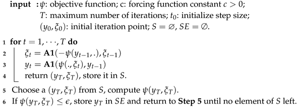
In this subsection, a min-max algorithm is proposed to solve problem (3.1). In our algorithm, we select different steps for the two variables y and

ξ

, which is different from one proposed in [21]. In addition, we extend the search directions of the algorithm to make the search faster and more suitable for different needs. Thus, our algorithm is an improvement of that in [21].

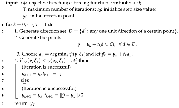
Direction set: The set D consist of finite unit vectors which can span

R^{n}

. Here, in order to reduce the computational cost, only consider some directions in D. For example, when

n = 2

, in this paper, let

D = {(1, 0), (\frac{\sqrt{3}}{2}, \frac{1}{2}), (1, 1),

(\frac{1}{2}, \frac{\sqrt{3}}{2}), (0, 1), (- \frac{1}{2}, \frac{\sqrt{3}}{2}), (- 1, 1), (- \frac{\sqrt{3}}{2}, \frac{1}{2}), (- 1, 0), (- \frac{\sqrt{3}}{2}, - \frac{1}{2})

(- 1, - 1)

(- \frac{1}{2}, - \frac{\sqrt{3}}{2}), (0, - 1), (\frac{1}{2}, - \frac{\sqrt{3}}{2}),

(1, - 1), (\frac{\sqrt{3}}{2}, - \frac{1}{2})}

Step length: Let initial step

t_{0} = 1

and

d_{k} = arg {min}_{y_{i}} ψ_{k} (y_{k} + t_{k} d, ξ_{k})

d \in D

. Let

{\tilde{y}}_{k} = y_{k} + t_{k} d_{k}

. If iteration is successful, i.e.,

ψ_{k} ({\tilde{y}}_{k}, ξ_{k})) < ψ_{k} (y_{k} + t_{k} d, ξ_{k}) - c t_{k}^{2}

for all

d \in D

(

c > 0

), then next step length value

t_{k + 1} = 1

; If iteration is unsuccessful, then

t_{k + 1} = ∥ \tilde{y} - y_{k} ∥ / 2

Algorithm 1: Min-Max Algorithm (Algorithm A)

Algorithm 2: Algorithm A1(ψ(), y₀)

Remark 3.1.

(i): It is worth noting that computations for $y_{t}$ and $ξ_{t}$ in $Algorithm$ $A$ are based on Algorithm $A 1$ .
(ii): The step strategy given in [21] is as follows: If iteration is successful, then $t_{k + 1} = min (t_{m a x}, γ t_{k})$ , $γ > 1$ , where $t_{m a x}$ is the largest step size; Otherwise $t_{k + 1} = \frac{1}{γ} t_{k}$ . In the following Subsection 3.3, we will give three numerical examples to show that the step strategy in $Algorithm A$ has better performance compared with that in [21].

3.3. Numerical Examples

In this subsection, there are some numerical examples with linear and nonlinear cost functions to illustrate

Algorithm

A

. In these numerical examples, both

Algorithm A

and algorithm proposed in [21] start from the same set of initial points. To make a fair comparison, all test problems are ran 5 times to reduce the impact of randomness.

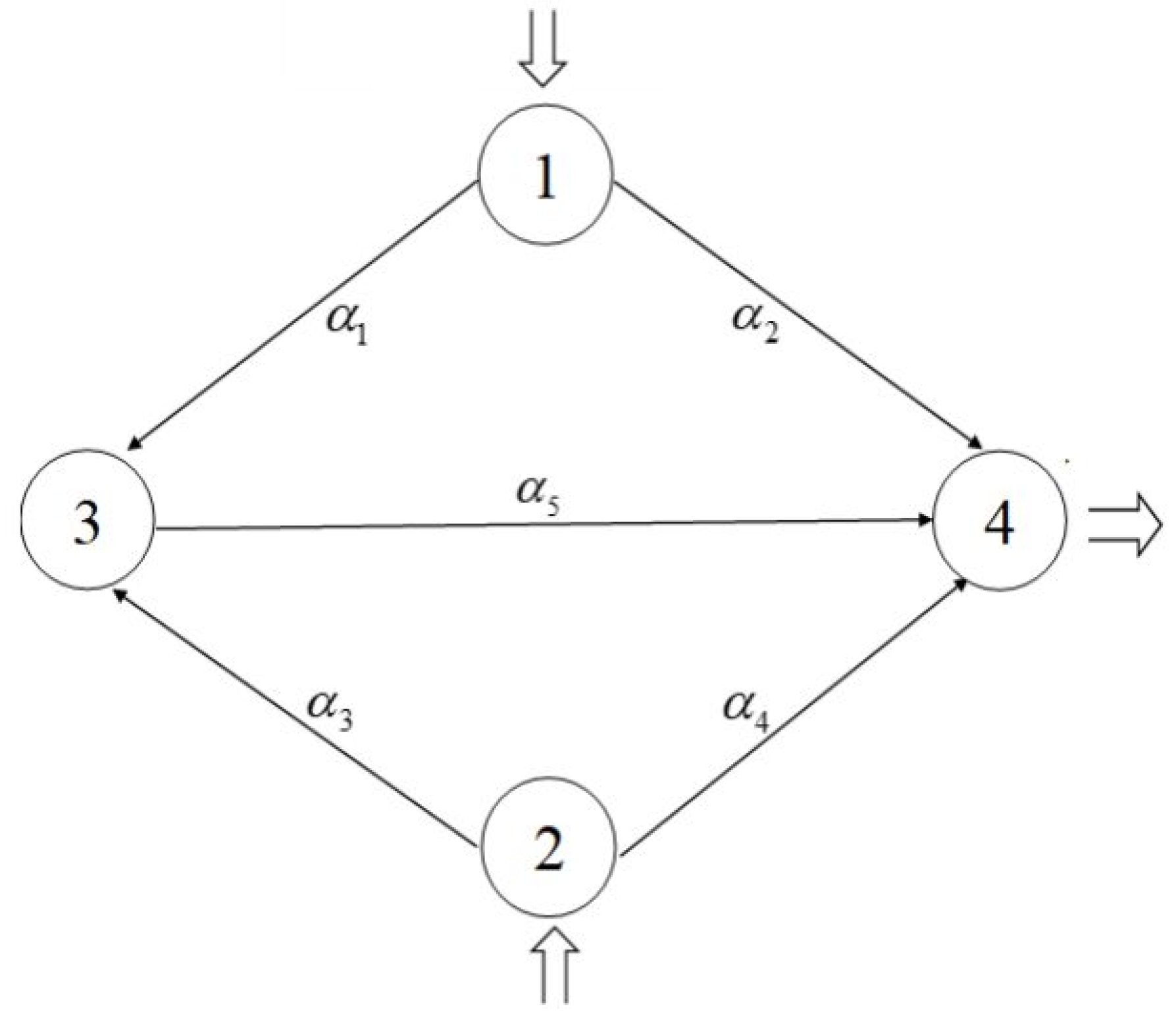
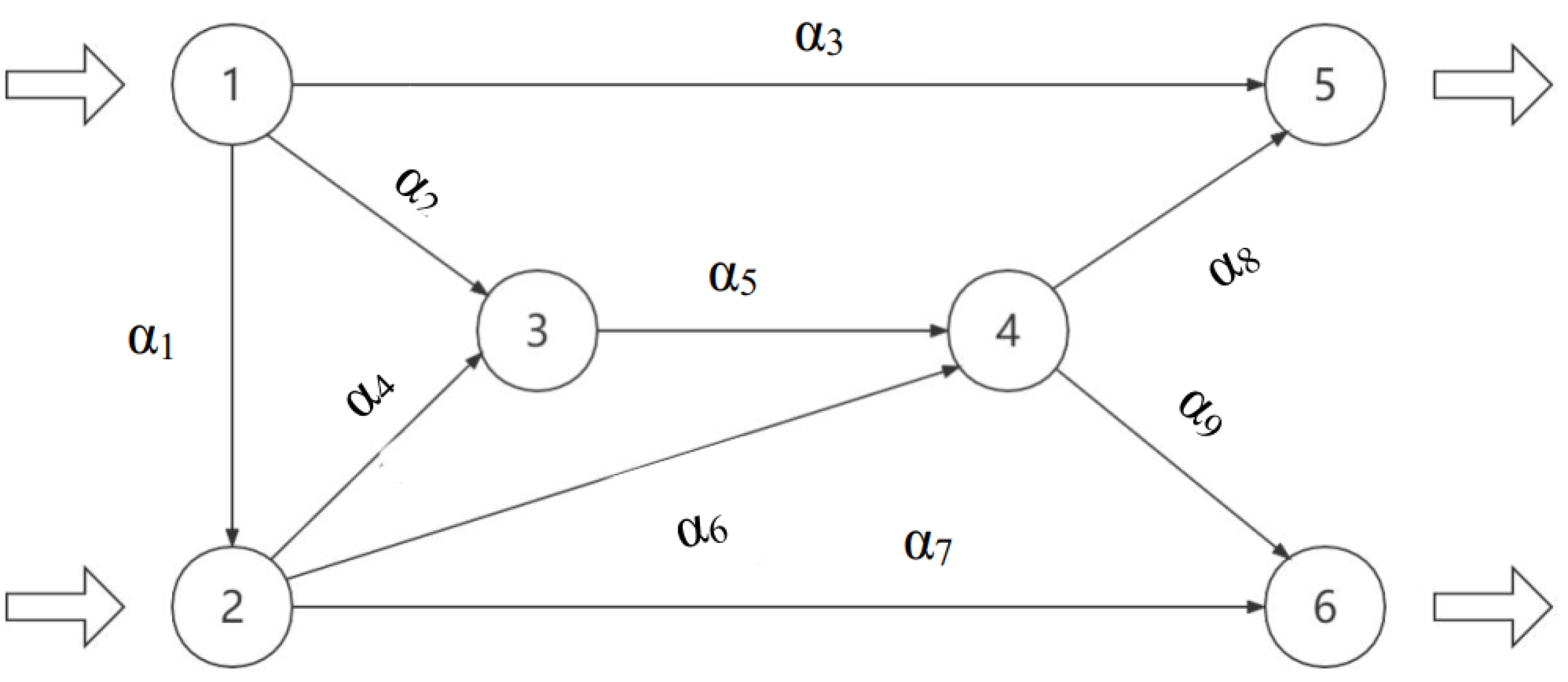
Example 3.1.

Consider a network problem depicted in Figure 1, where

N = {1, 2}, W = {ω} = \{(1, 2)\}, E = {α_{1}, α_{2}}, D = d_{ω} = 30

. Two criteria: travel time and travel cost. The cost functions of arcs and constraints of paths are given as bellow:

t_{1, α_{1}} (y, ξ) = y_{1}^{2} + 2 y_{1} y_{2} + y_{2} - ξ_{1}

t_{2, α_{1}} (y, ξ) = y_{1} + y_{2}^{2};

t_{1, α_{2}} (y, ξ) = y_{1}^{2} + 10 y_{2} y_{2}

t_{2, α_{2}} (y, ξ) = 7 y_{1} + 6 y_{2}^{2} - 6 ξ_{2}

l_{p_{1}} = 0, l_{p_{2}} = 0; u_{p_{1}} = 30, u_{p_{2}} = 30 .

Then, we have

c_{p_{1}} (y, ξ) = (\begin{matrix} y_{1}^{2} + 2 y_{1} y_{2} + y_{2} - ξ_{1} \\ y_{1} + y_{2}^{2} \end{matrix}), c_{p_{2}} (y, ξ) = (\begin{matrix} y_{1}^{2} + 10 y_{2} y_{2} \\ 7 y_{1} + 6 y_{2}^{2} - 6 ξ_{2} \end{matrix}) .

where

ξ_{1} \in [0, 1]

and

ξ_{2} \in [0, 1]

. Initial feasible flows and a subset of robust vector equilibrium flows are obtained in

23.12 s

. The results are shown in the Table 1. However, if we use step calculational method in [21], then it takes 25.86s and the obtain the same robust vector equilibrium flows with our algorithm.

Table 1. Computational results of

Algorithm

A

Table 1. Computational results of

Algorithm

A

Initial feasible flows	Robust vector equilibrium flows
$(0.00, 30.00)$ $(3.75, 26.25)$	$(25.00, 5.00)$ $(25.75, 4.25)$
$(11.25, 18.75)$ $(11.25, 18.75)$	$(25.50, 4.50)$ $(25.25, 4.75)$
$(15.00, 15.00)$ $(18.75, 11.25)$	$(25.00, 5.00)$ $(25.75, 4.25)$
$(22.50, 7.50)$ $(26.25, 3, 75)$	$(25.50, 4.50)$ $(26.25, 3.75)$
$(30.00, 0.00)$	$(30.00, 0.00)$

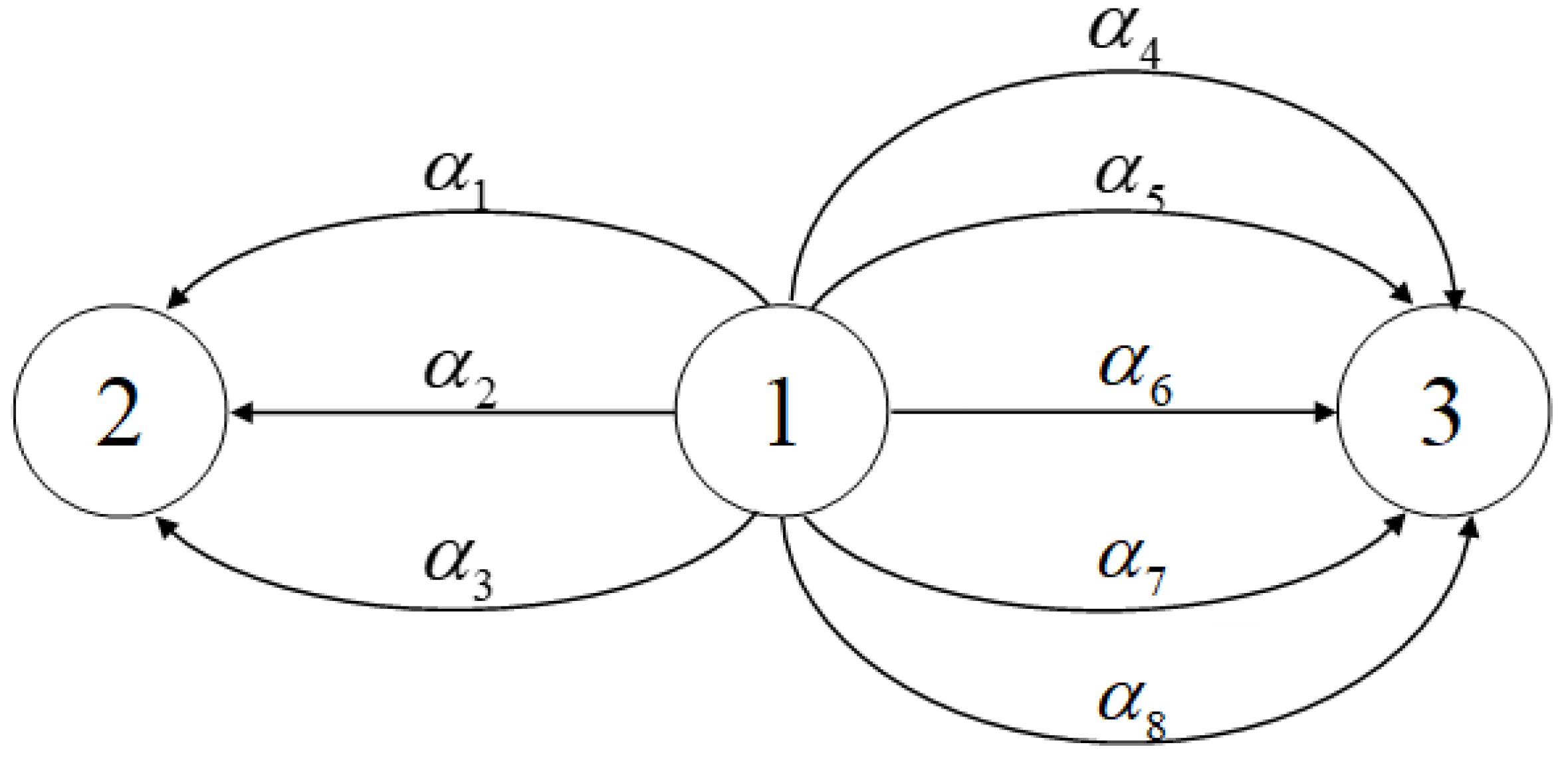
Example 3.2.

Consider the network problem depicted in Figure 2, where

N = {1, 2, 3, 4}, W = \{(1, 4), (2, 4)\}

, two O-D pairs

ω_{1}, ω_{2}

E = {α_{1}, α_{2}, α_{3}, α_{4}, α_{5}}, p_{1} = (α_{1} α_{5}), p_{2} = (α_{2}), p_{3} = (α_{3} α_{5}), p_{4} = (α_{4}), D = {d_{ω_{1}}, d_{ω_{2}}} = {55, 35}

. Two criteria: travel time and travel cost. Constrains of paths are given as follows:

l_{p_{1}} = 0, l_{p_{2}} = 0, l_{p_{3}} = 0, l_{p_{4}} = 0;

u_{p_{1}} = 55, u_{p_{2}} = 55, u_{p_{3}} = 35, u_{p_{4}} = 35 .

The cost functions of arcs are defined as follows:

t_{α_{1}} (y, ξ) = (\begin{matrix} y_{1}^{2} + 2 y_{2} + y_{3}^{2} + y_{4}^{2} + 1 \\ 2 y_{1} + y_{2}^{2} + 2 y_{3} + y_{4} + \frac{3}{2} - 6 ξ_{1} \end{matrix}), t_{α_{2}} (y, ξ) = (\begin{matrix} 2 y_{1} + 3 y_{2} + 5 y_{3} + y_{4} + 1 + ξ_{2} \\ 2 y_{1} y_{2} + y_{2} + y_{3}^{2} + y_{4} + \frac{1}{2} \end{matrix}),

t_{α_{3}} (y, ξ) = (\begin{matrix} 2 y_{1} + y_{2} + y_{3}^{2} + y_{4} + \frac{3}{2} + 3 ξ_{3} \\ y_{3}^{2} + 5 y_{4} + 1 \end{matrix}), t_{α_{4}} (y, ξ) = (\begin{matrix} 2 y_{2} + 3 y_{3} y_{4} + y_{4}^{2} + 1 \\ y_{1}^{2} + y_{2} + y_{4} + \frac{1}{2} - 8 ξ_{4} \end{matrix}), t_{α_{5}} (y) = (\begin{matrix} y_{1} + y_{2} \\ y_{3} + y_{4} \end{matrix}) .

Then, we have

c_{p_{1}} (y, ξ) = (\begin{matrix} y_{1}^{2} + y_{1} + 3 y_{2} + y_{3}^{2} + y_{4}^{2} + 1 \\ 2 y_{1} + y_{2}^{2} + 3 y_{3} + 2 y_{4} + 1.5 - 6 ξ_{1} \end{matrix}), c_{p_{2}} (y, ξ) = (\begin{matrix} 2 y_{1} + 3 y_{2} + 5 y_{3} + y_{4} + 1 + ξ_{2} \\ 2 y_{1} y_{2} + y_{2} + y_{3}^{2} + y_{4} + 0.5 \end{matrix})

c_{p_{3}} (y, ξ) = (\begin{matrix} 3 y_{1} + 2 y_{2} + y_{3}^{2} + y_{4} + 1.5 + 3 ξ_{3} \\ y_{3}^{2} + y_{3} + 6 y_{4} + 1 \end{matrix}), c_{p_{4}} (y, ξ) = (\begin{matrix} 2 y_{2} + 3 y_{3} y_{4} + y_{4}^{2} + 1 \\ y_{1}^{2} + y_{2} + 8 y_{4} + 0.5 - 8 ξ_{4} \end{matrix})

where

ξ_{i} \in [0, 1], i = 1, 2, 3, 4

. Initial feasible flows and a subset of robust vector equilibrium flows are obtained in

40.56 s

. The results are shown in the Table 2. The time cost of

Algorithm A

4 %

lower than that of the step calculation method in [21].

Table 2. Computational results of

Algorithm

A

Table 2. Computational results of

Algorithm

A

Initial feasible flows	Robust vector equilibrium flows
$(0.00, 55.00, 0.00, 35.00)$ $(5.00, 50.00, 5.00, 30.00)$	$(27.00, 28.00, 27.00, 8.00)$ $(27.00, 28.00, 27.00, 8.00)$
$(10.00, 45.00, 10.00, 25.00)$ $(15.00, 40.00, 15.00, 20.00)$	$(27.00, 28.00, 27.00, 8.00)$ $(27.00, 28.00, 27.00, 8.00)$
$(20.00, 35.00, 20.00, 15.00)$ $(25.00, 30.00, 25.00, 10.00)$	$(27.00, 28.00, 27.00, 8.00)$ $(29.00, 26.00, 29.00, 6.00)$
$(30.00, 25.00, 30.00, 5.00)$ $(35.00, 20.00, 35.00, 0.00)$	$(29.00, 26.00, 29.00, 6.00)$

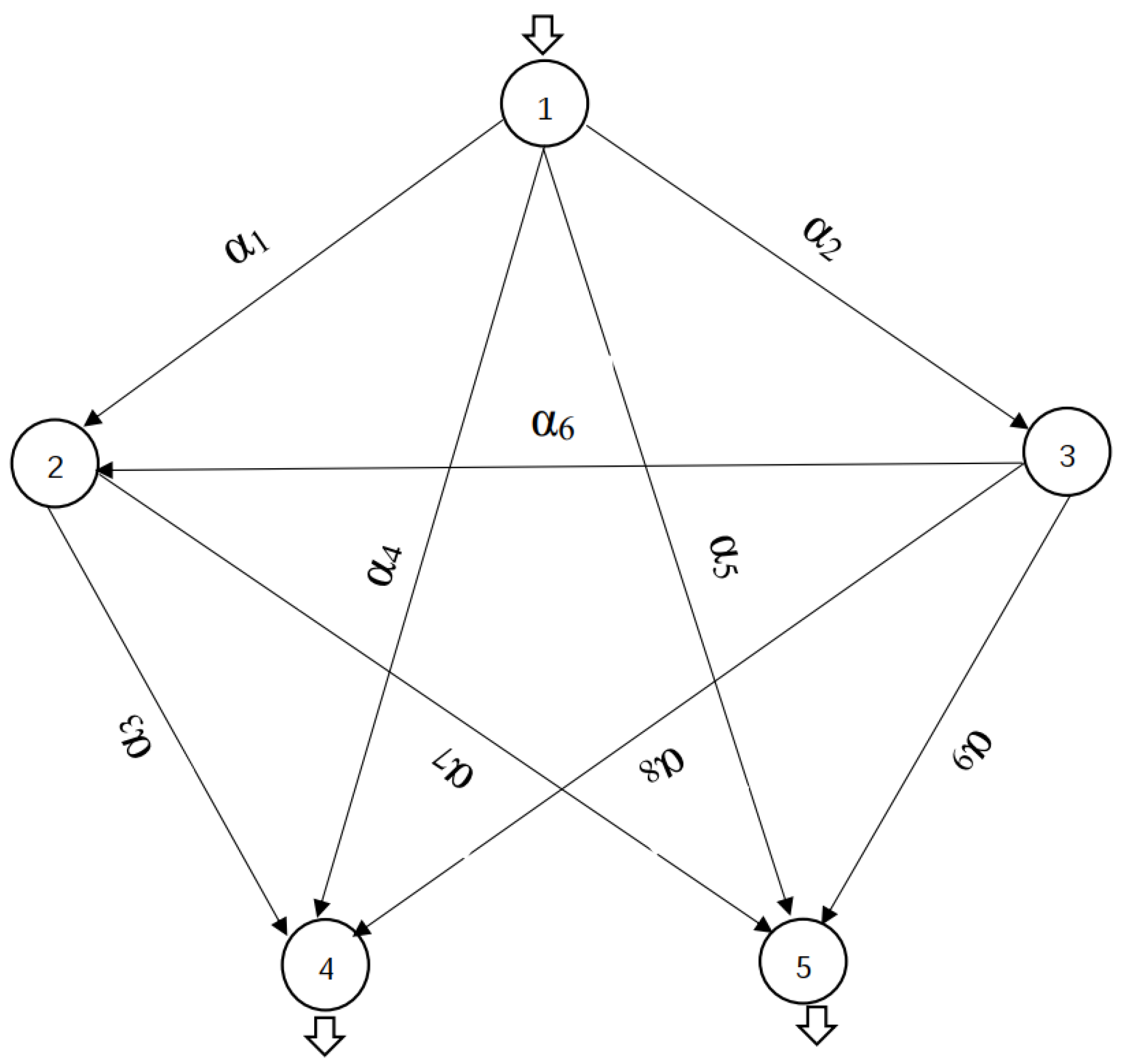
Example 3.3.

Consider the network problem depicted in Figure 3, where

N = {1, 2, 3, 4, 5, 6}, W = {ω_{1}, ω_{2}} = \{(1, 5), (2, 6)\}, E = {α_{1}, α_{2}, α_{3}, α_{4}, α_{5}, α_{6}, α_{7}, α_{8}, α_{9}}, D = {d_{ω_{1}}, d_{ω_{2}}}, d_{ω_{1}} = 25, d_{ω_{2}} = 20

, two criteria: travel time and travel cost.

P_{ω} = {p_{1}, p_{2}, p_{3}, p_{4}, p_{5}, p_{6}, p_{7}}

, where

P_{ω_{1}} = {p_{1}, p_{2}, p_{3}, p_{4}}

P_{ω_{2}} = {p_{5}, p_{6}, p_{7}}, p_{1} = (α_{3}), p_{2} = (α_{2} α_{5} α_{8}), p_{3} = (α_{1} α_{4} α_{5} α_{8}), p_{4} = (α_{1} α_{6} α_{8}), p_{5} = (α_{7}), p_{6} = (α_{6} α_{9}), p_{7} = (α_{4} α_{5} α_{9})

The constrains of paths and cost functions are given as follows:

l_{p_{1}} = 0, l_{p_{2}} = 0, l_{p_{3}} = 0, l_{p_{4}} = 0, l_{p_{5}} = 0, l_{p_{6}} = 0, l_{p_{7}} = 0;

u_{p_{1}} = 25, u_{p_{2}} = 25, u_{p_{3}} = 25, u_{p_{4}} = 25, u_{p_{5}} = 20, u_{p_{6}} = 20, u_{p_{7}} = 20 .

t_{1, α_{1}} (_{α_{1}}, ξ) = 4 z_{α_{1}} + 50 - 2 ξ_{3}, t_{2, α_{1}} (z_{α_{1}}, ξ) = z_{α_{1}}^{2} + 90 - 2 ξ_{3};

t_{1, α_{2}} (z_{α_{2}}, ξ) = 2 z_{α_{2}} + 20 - ξ_{2} + 4 ξ_{6}, t_{2, α_{2}} (z_{α_{2}}, ξ) = 3 z_{α_{2}}^{2} + 10;

t_{1, α_{3}} (z_{α_{3}}, ξ) = 4 z_{α_{3}}^{2} + 100 + ξ_{1}, t_{2, α_{3}} (z_{α_{3}}, ξ) = 2 z_{α_{3}}^{2} + 110 + 6 ξ_{1};

t_{1, α_{4}} (z_{α_{4}}, ξ) = 2 z_{α_{4}} + 10 + ξ_{2}, t_{2, α_{4}} (z_{α_{4}}, ξ) = z_{α_{4}}^{2} + 30 - ξ_{2} + ξ_{3};

t_{1, α_{5}} (z_{α_{5}}, ξ) = 2 z_{α_{5}}^{2} + 10 - ξ_{2}, t_{2, α_{5}} (z_{α_{5}}, ξ) = z_{α_{5}}^{2} + 20 + ξ_{2};

t_{1, α_{6}} (z_{α_{6}}, ξ) = 5 z_{α_{6}}^{2} + 430 + 2 ξ_{3} + ξ_{4}, t_{2, α_{6}} (z_{α_{6}}, ξ) = 2 z_{α_{6}} + 530 + 2 ξ_{3} - ξ_{4};

t_{1, α_{7}} (z_{α_{7}}, ξ) = 2 z_{α_{2}}^{2} + 100 + 5 ξ_{5}, t_{2, α_{7}} (z_{α_{7}}, ξ) = 3 z_{α_{7}} + 300;

t_{1, α_{8}} (z_{α_{8}}, ξ) = z_{α_{8}}^{2} + 20, t_{2, α_{8}} (z_{α_{8}}, ξ) = 2 z_{α_{8}}^{2} + 10;

t_{1, α_{9}} (z_{α_{9}}, ξ) = z_{α_{9}}^{2} + 30 - 4 ξ_{6}, t_{2, α_{9}} (z_{α_{9}}, ξ) = 2 z_{α_{9}} + 10 + 2 ξ_{7} - ξ_{3};

where

z_{α_{i}} (i = 1, 2, . . ., 9)

denotes the flow on arc

α_{i}

Then we have

c_{p_{1}} (y, ξ) = (\begin{matrix} 4 y_{1}^{2} + 100 + ξ_{1} \\ 2 y_{1}^{2} + 110 + 6 ξ_{1} \end{matrix}), c_{p_{2}} (y, ξ) = (\begin{matrix} 2 y_{2} + 2 {(y_{3} + y_{4} + y_{7})}^{2} + {(y_{3} + y_{6} + y_{7})}^{2} + 50 - 2 ξ_{2} \\ 3 y_{2}^{2} + {(y_{3} + y_{4} + y_{7})}^{2} + 2 {(y_{3} + y_{6} + y_{7})}^{2} + 40 + ξ_{2} \end{matrix})

c_{p_{3}} (y, ξ) = (\begin{matrix} 4 (y_{6} + y_{7}) + 2 (y_{4} + y_{7}) + 2 {(y_{3} + y_{4} + y_{7})}^{2} + {(y_{3} + y_{6} + y_{7})}^{2} + 90 - 2 ξ_{3} \\ {(y_{6} + y_{7})}^{2} + {(y_{4} + y_{7})}^{2} + {(y_{3} + y_{4} + y_{7})}^{2} + 2 {(y_{3} + y_{6} + y_{7})}^{2} + 150 - ξ_{3} \end{matrix})

c_{p_{4}} (y, ξ) = (\begin{matrix} 4 (y_{6} + y_{7}) + 5 {(y_{4} + y_{5})}^{2} + {(y_{3} + y_{6} + y_{7})}^{2} + 500 + ξ_{4} \\ {(y_{6} + y_{7})}^{2} + 2 (y_{4} + y_{5}) + 2 {(y_{3} + y_{6} + y_{7})}^{2} + 630 - ξ_{4} \end{matrix})

c_{p_{5}} (y, ξ) = (\begin{matrix} 2 y_{2}^{2} + 100 + 5 ξ_{5} \\ 3 y_{5} + 300 \end{matrix}), c_{p_{6}} (y, ξ) = (\begin{matrix} 5 {(y_{4} + y_{5})}^{2} + {(y_{5} + y_{6})}^{2} + 460 - 4 ξ_{6} \\ 2 (y_{4} + y_{5}) + 2 (y_{5} + y_{6}) + 540 \end{matrix})

c_{p_{7}} (y, ξ) = (\begin{matrix} 2 (y_{4} + y_{7}) + 2 {(y_{3} + y_{4} + y_{7})}^{2} + {(y_{5} + y_{6})}^{2} + 50 \\ {(y_{4} + y_{7})}^{2} + {(y_{3} + y_{4} + y_{7})}^{2} + 2 {(y_{5} + y_{6})}^{2} + 60 + 2 ξ_{7} \end{matrix})

where

ξ_{i} \in [0, 1], i = 1, 2, 3, 4, 5, 6, 7

. Initial feasible flows and a subset of robust vector equilibrium flows are obtained in

538.47 s

. The results are shown in the Table 3. The algorithm proposed [21] obtain the same robust vector equilibrium flows but its time cost is 548.32s.

Table 3. Computational results of

Algorithm

A

Table 3. Computational results of

Algorithm

A

Initial feasible flows	Robust vector equilibrium flows
$(0, 0, 0, 25, 0, 0, 20)$ $(0, 0, 25, 0, 0, 0, 20)$	$(9, 7, 9, 0, 19, 0, 1)$ $(12, 13, 0, 0, 8, 0, 12)$
$(0, 25, 0, 0, 0, 0, 20)$ $(25, 0, 0, 0, 0, 0, 20)$	$(15, 10, 0, 0, 9, 0, 11)$ $(15, 10, 0, 0, 9, 0, 11)$
$(0, 0, 0, 25, 0, 20, 0)$ $(0, 0, 25, 0, 0, 20, 0)$	$(12, 8, 5, 0, 15, 0, 5)$ $(15, 10, 0, 0, 9, 0, 11)$
$(0, 25, 0, 0, 0, 20, 0)$ $(25, 0, 0, 0, 0, 20, 0)$	$(9, 7, 9, 0, 19, 0, 1)$ $(12, 13, 0, 0, 8, 0, 12)$
$(0, 0, 0, 25, 20, 0, 0)$ $(0, 0, 25, 0, 20, 0, 0)$	$(11, 7, 7, 0, 18, 0, 2)$
$(0, 25, 0, 0, 20, 0, 0)$ $(25, 0, 0, 0, 20, 0, 0)$

4. Smoothing Method for Robust Vector equilibrium with Worst Case

In this section, we propose a smoothing method to calculate a subset of robust vector equilibrium with respect to worst case. The algorithm is denoted

Algorithm

B

. To generalize a subset of robust vector equilibrium flows with respect to worst case, we use a two-step strategy. The first step is to construct an equivalent optimization problem with the help of a variant version of ReLU activation function for finding robust weak vector equilibrium flows with respect to worst case. The second step is to judge whether robust weak vector equilibrium flows with respect to worst case is robust vector equilibrium flows with respect to worst case by an equivalent optimization problem using the vector version of Heaviside step function.

Define a function

r : R \to R

and give its vector version function

R

R^{n} \to R^{m}

as follows:

r (a) = {(m a x {0, a})}^{2} .

R (x) = (\prod_{i = 1}^{n} r (x_{i})) e,

In addition, the Heaviside Step function

h_{+} : R \to R

and its vector version function

H_{+} : R^{n} \to R^{m}

are also given below.

h_{+} (a) = \{\begin{matrix} 1, & if a \geq 0, \\ 0, & o t h e r w i s e . \end{matrix}

H_{+} (x) = (\prod_{i = 1}^{n} h_{+} (x_{i})) e, \forall x \in R^{m} .

4.1. Associated Optimization Problems

In this subsection, we construct an optimization problem whose solution is equivalent to a robust weak vector equilibrium flow with respect to worst case. For

y \in Ω

, we define

ϕ (y) : = \sum_{ω \in W} \sum_{p_{k}, p_{j} \in P_{ω}} (y_{p_{k}} - l_{p_{k}}) (u_{p_{j}} - y_{p_{j}}) {(C_{p_{k}} (y) - C_{p_{j}} (y))}^{⊤} R [C_{p_{k}} (y) - C_{p_{j}} (y)] .

Proposition 4.1.

Let

\bar{y}

be a feasible flow. The following statements are equivalent.

(i): $\bar{y}$ is a robust weak vector equilibrium with respect to worst case;
(ii): $\bar{y}$ is an optimal solution of the problem, denoted

$\begin{matrix} min ϕ (\bar{y}) \\ s . t . y \in Ω . \end{matrix}$

(4.1)

and the optimal value $ϕ (\bar{y})$ is equal to zero.

Proof.

We first prove implication

(i) \Rightarrow (i i)

. It is not hard to see

ϕ (y) \geq 0

for every

y \in Ω

. Thus, if

\bar{y}

is a robust weak vector equilibrium with respect to worst case, in order to deduce (ii), it suffices to prove

ϕ (\bar{y}) = 0

. In addition, for every

p_{k} \in p_{ω}, ω \in W

, consider the term

Q_{p} = \sum_{ω \in W} \sum_{p_{k}, p_{j} \in P_{ω}} (y_{p_{k}} - l_{p_{k}}) (u_{p_{j}} - y_{p_{j}}) {(C_{p_{k}} (y) - C_{p_{j}} (y))}^{⊤} R [C_{p_{k}} (y) - C_{p_{j}} (y)] .

C_{p_{k}} (\bar{y}) - C_{p_{j}} (\bar{y}) ≻ 0_{R^{m}}

, for some

p_{j} \in P_{ω}

, then by definition, either

{\bar{y}}_{p_{k}} = l_{p_{k}}

{\bar{y}}_{p_{j}} = u_{p_{j}}

; If

C_{p_{k}} (\bar{y}) - C_{p_{j}} (\bar{y}) = 0_{R^{m}}

, for some

p_{j} \in P_{ω}

, we also get

Q_{p} = 0

; If

C_{p_{k}} (\bar{y}) - C_{p_{j}} (\bar{y}) ≺ 0_{R^{m}}

, then

R [C_{p_{k}} (y) - C_{p_{j}} (y)] = 0_{R^{m}}

and so

Q_{p} = 0

. As a result, one has

ϕ (\bar{y}) = 0

Conversely, assume that

\bar{y}

is an optimal solution of problem (4.1) and

ϕ (\bar{y}) = 0

. Then we have

Q_{p} = 0

for all

p \in P

. If there exists some

p_{k}, p_{j} \in p_{ω}, ω \in W

such that

C_{p_{k}} (\bar{y}) - C_{p_{j}} (\bar{y}) ≻ 0_{R^{m}}

, then

{(C_{p_{k}} (y) - C_{p_{j}} (y))}^{'} R [C_{p_{k}} (y) - C_{p_{j}} (y) ≻ 0_{R^{m}}

and so either

{\bar{y}}_{p_{k}} = l_{p_{k}}

{\bar{y}}_{p_{j}} = u_{p_{j}}

Q_{p} = 0

. Consequently, we deduce that

\bar{y}

is a robust weak vector equilibrium with respect to worst case. □

For

y \in Ω

, we define

φ (y) = \sum_{ω \in W} \sum_{p_{k}, p_{j} \in P_{ω}} (y_{p_{k}} - l_{p_{k}}) (u_{p_{j}} - y_{p_{j}}) {(C_{p_{k}} (y) - C_{p_{j}} (y))}^{⊤} H_{+} [C_{p_{k}} (y) - C_{p_{j}} (y)] .

Then by using the same method of proof, we may establish a similar result for robust vector equilibrium with respect to worst case.

Proposition 4.2.

Let

\bar{y}

be a feasible flow. The following statements are equivalent.

(i): $\bar{y}$ is a robust vector equilibrium with respect to worst case.
(ii): $\bar{y}$ is an optimal solution of the problem, denoted

$\begin{matrix} min φ (y) \\ s . t . y \in Ω . \end{matrix}$

(4.2)

and the optimal value $φ (\bar{y})$ is equal to zero.

4.2. Description of the Algorithm

Algorithm

B

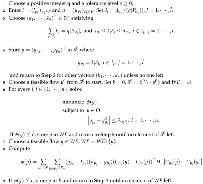
is mainly based on ideas of Proposition 4.1 and Proposition 4.2.

Steps 1 - 4

create a subset of feasible flows with the initial conditions, denoted

S^{0}

, with which

Steps 4 - 6

will start.

Steps 5 - 6

are aim at solving problem (4.1) given in Proposition 4.1 by using first-order optimization methods, and then a subset of robust weak vector equilibrium flows with respect to worst case is gained.

Steps 7 - 9

focus on solving problem (4.2) given in Proposition 4.2, and then a subset of the robust vector equilibrium flows with respect to worst case is generated.

Assume that

W

consists of

\tilde{l}

elements

ω_{1}, . . ., ω_{\tilde{l}}

in the network and for each pair

ω_{i}

. Let

I_{j} = \{i \in \{1, . . ., n\} : p_{i} \in P_{w_{j}}\}

. Denote

W E

by the subset of robust weak vector equilibrium flows with respect to worst case and E by the subset of robust vector equilibrium flows with respect to worst case.

Algorithm 3: Robust Vector Equilibrium Algorithm (Denoted Algorithm B)

4.3. Numerical Examples

Example 4.1.

Consider the network problem depicted in Figure 4, where

N = {1, 2, 3, 4, 5}, W = {ω_{1}, ω_{2}} = \{(1, 4), (1, 5)\}, E = {α_{1}, α_{2}, α_{3}, α_{4}, α_{5}, α_{6}, α_{7}, α_{8}, α_{9}}, D = {d_{ω_{1}}, d_{ω_{2}}}, d_{ω_{1}} = 25, d_{ω_{2}} = 20

, two criteria: travel time and travel cost,

P_{ω} = {p_{1}, p_{2}, p_{3}, p_{4}, p_{5}, p_{6}, p_{7}}

, where

P_{ω_{1}} = {p_{1}, p_{2}, p_{3}, p_{4}}

P_{ω_{2}} = {p_{5}, p_{6}, p_{7}}

Assume that

l_{p_{1}} = l_{p_{2}} = l_{p_{3}} = l_{p_{4}} = l_{p_{5}} = l_{p_{6}} = l_{p_{7}} = l_{p_{8}} = 0;

u_{p_{1}} = 100, u_{p_{2}} = 100, u_{p_{3}} = 100, u_{p_{4}} = 200, u_{p_{5}} = 100, u_{p_{6}} = 120, u_{p_{7}} = 150, u_{p_{8}} = 100;

t_{1, α_{1}} (y, ξ) = y_{1}^{2} + y_{2}^{2} + y_{3}^{3} + ξ_{1}, t_{2, α_{1}} (y, ξ) = 2 y_{1} + 5 y_{2} + 3 y_{3} + y_{4} - 2 ξ_{1};

t_{1, α_{2}} (y, ξ) = 8 y_{1} y_{2} + y_{2}^{2} + y_{7} + y_{8} + 4 ξ_{2}, t_{2, α_{2}} (y, ξ) = y_{2} + 10 y_{3} + 2 y_{7} + y_{8} + 2 ξ_{2};

t_{1, α_{3}} (y, ξ) = y_{1} + y_{2}^{2} + y_{3}^{3} + y_{5} + y_{6} - 3 ξ_{3}, t_{2, α_{3}} (y, ξ) = 10 y_{3}^{3} + 2 y_{5} + ξ_{3};

t_{1, α_{4}} (y, ξ) = y_{1} + y_{2} + y_{4}^{3} + y_{5}^{2} + y_{8}^{3} + ξ_{4}, t_{2, α_{4}} (y, ξ) = y_{1} + 2 y_{4} + y_{6} y_{5} + 15 y_{8};

t_{1, α_{5}} (y, ξ) = y_{1} + y_{3} + y_{4}^{3} + y_{5}^{2} + y_{6}^{2}, t_{2, α_{5}} (y, ξ) = y_{1} + 5 y_{3} + 5 y_{5} + 3 y_{6} + 12 y_{7} + 4 ξ_{5};

t_{1, α_{6}} (y, ξ) = y_{3} + y_{4} + y_{5} + y_{6}^{3} - 3 ξ_{6}, t_{2, α_{6}} (y, ξ) = 3 y_{3} + 10 y_{5} + y_{6} + 2 y_{8} - 2 ξ_{6};

t_{1, α_{7}} (y, ξ) = y_{2} + 8 y_{4}^{2} + y_{5} + y_{7}^{3} + 2 ξ_{7}, t_{2, α_{7}} (y, ξ) = y_{1} + y_{2} + 5 y_{4} + 3 y_{7};

t_{1, α_{8}} (y, ξ) = y_{1} + y_{3} + 8 y_{6} y_{7} + y_{8}^{2} + ξ_{8}, t_{2, α_{8}} (y, ξ) = y_{1} + y_{3} + 10 y_{5}^{3} + y_{8} - ξ_{8},

where

ξ_{i} \in [0, 1], i = 1, 2, 3, 4, 5, 6, 7, 8

. Then, we have

C_{p_{1}} (y) = (\begin{matrix} y_{1}^{2} + y_{2}^{2} + y_{3}^{3} + 1 \\ 2 y_{1} + 5 y_{2} + 3 y_{3} + y_{4} \end{matrix}), C_{p_{2}} (y) = (\begin{matrix} 8 y_{1} y_{2} + y_{2}^{2} + y_{7} + y_{8} + 4 \\ y_{2} + 10 y_{3} + 2 y_{7} + y_{8} + 2 \end{matrix})

C_{p_{3}} (y) = (\begin{matrix} y_{1} + y_{2}^{2} + y_{3}^{3} + y_{5} + y_{6} \\ 10 y_{3}^{3} + 2 y_{5} + 1 \end{matrix}), C_{p_{4}} (y) = (\begin{matrix} y_{1} + y_{2} + y_{4}^{3} + y_{5}^{2} + y_{8}^{3} + 1 \\ y_{1} + 2 y_{4} + y_{6} y_{5} + 15 y_{8} \end{matrix})

C_{p_{5}} (y) = (\begin{matrix} y_{1} + y_{3} + y_{4}^{3} + y_{5}^{2} + y_{6}^{2} \\ y_{1} + 5 y_{3} + 5 y_{5} + 3 y_{6} + 12 y_{7} + 4 \end{matrix}), C_{p_{6}} (y) = (\begin{matrix} y_{3} + y_{4} + y_{5} + y_{6}^{3} \\ 3 y_{3} + 10 y_{5} + y_{6} + 2 y_{8} \end{matrix})

C_{p_{7}} (y) = (\begin{matrix} y_{2} + 8 y_{4}^{2} + y_{5} + y_{7}^{3} + 2 \\ y_{1} + y_{2} + 5 y_{4} + 3 y_{7} \end{matrix}), C_{p_{8}} (y) = (\begin{matrix} y_{1} + y_{3} + 8 y_{6} y_{7} + y_{8}^{2} + 1 \\ y_{1} + y_{3} + 10 y_{5}^{3} + y_{8} \end{matrix})

Choosing

q = 2

, we have 32 feasible flows and 2 robust (weak) vector equilibrium flows with respect to worst case are obtained in

0.18 s

. Robust (weak) vector equilibrium flows with respect to worst case are shown in the Table 4. However, using algorithm proposed in [19], it will take

13.826 s

to obtain 5 robust vector equilibrium flows with respect to worst case which are shown in Table 5.

Table 4. Computational results of

Algorithm

B

Table 4. Computational results of

Algorithm

B

Robust weak vector equilibrium flows (worst case)	Robust vector equilibrium flows (worst case)
$(100, 100, 100, 145.125, 0, 120, 134.875, 100)$	$(100, 100, 100, 145.125, 0, 120, 134.875, 100)$
$(100, 100, 100, 150, 0, 120, 130, 100)$	$(100, 100, 100, 150, 0, 120, 130, 100)$

Table 5. Computational results of algorithm in [19].

Robust vector equilibrium flows (worst case)

(100, 100, 100, 30, 100, 120, 150, 100)

(100, 100, 100, 50, 100, 120, 130, 100)

(100, 100, 100, 100, 100, 120, 80, 100)

(100, 100, 100, 150, 100, 120, 30, 100)

(100, 100, 100, 200, 100, 100, 100, 0)

Example 4.2.

Consider the network problem depicted in Figure 5, where

N = {1, 2, 3, 4, 5}, W = {ω_{1}, ω_{2}} = \{(1, 4), (1, 5)\}, E = {α_{1}, α_{2}, α_{3}, α_{4}, α_{5}, α_{6}, α_{7}, α_{8}, α_{9}}, D = {d_{ω_{1}}, d_{ω_{2}}}

with

d_{ω_{1}} = 25

d_{ω_{2}} = 20

, two criteria: travel time and travel cost,

P_{ω} = {p_{1}, p_{2}, p_{3}, p_{4}, p_{5}, p_{6}, p_{7}}

, where

P_{ω_{1}} = {p_{1}, p_{2}, p_{3}, p_{4}}

P_{ω_{2}} = {p_{5}, p_{6}, p_{7}}

p_{1} = (α_{4}), p_{2} = (α_{2} α_{8}), p_{3} = (α_{2} α_{6} α_{3}), p_{4} = (α_{1} α_{3}), p_{5} = (α_{5}), p_{6} = (α_{2} α_{9}), p_{7} = (α_{1} α_{7})

. Let

l_{1} = 0, l_{2} = 0, l_{3} = 0, l_{4} = 0, l_{5} = 0, l_{6} = 0, l_{7} = 0;

u_{1} = 15, u_{2} = 20, u_{3} = 15, u_{4} = 10, u_{5} = 15, u_{6} = 10, u_{7} = 15 .

Now, we given the cost function of arcs as follow:

t_{α_{1}} (y, ξ) = (\begin{matrix} 4 (y_{6} + y_{7}) + 2 {(y_{3} + y_{4} + y_{7})}^{2} + 300 - 2 ξ_{1} \\ {(y_{6} + y_{7})}^{2} + {(y_{3} + y_{4} + y_{7})}^{2} + 330 - ξ_{1} \end{matrix}), t_{α_{2}} (y, ξ) = (\begin{matrix} 2 {(y_{3} + y_{4} + y_{7})}^{2} + 50 + ξ_{2} \\ {(y_{3} + y_{4} + y_{7})}^{2} \end{matrix})

t_{α_{3}} (y, ξ) = (\begin{matrix} 2 (y_{3} + y_{7}) + 2 {(y_{4} + y_{7})}^{2} + 300 + 2 ξ_{1} + ξ_{6} \\ {(y_{3} + y_{7})}^{2} + 2 (y_{4} + y_{7}) + 100 + ξ_{1} - ξ_{3} \end{matrix}), t_{α_{4}} (y, ξ) = (\begin{matrix} 4 y_{1}^{2} + 100 + ξ_{4} \\ 2 y_{1}^{2} + 110 + 6 ξ_{4} \end{matrix})

t_{α_{5}} (y, ξ) = (\begin{matrix} 2 y_{2}^{2} + 100 + 5 ξ_{5} \\ 3 y_{2} + y_{5} + 300 \end{matrix}), t_{α_{6}} (y, ξ) = (\begin{matrix} {(y_{3} + y_{6} + y_{7})}^{2} - 260 - ξ_{6} - ξ_{2} \\ 2 {(y_{3} + y_{6} + y_{7})}^{2} + 50 - ξ_{1} \end{matrix})

t_{α_{7}} (y, ξ) = (\begin{matrix} 2 (y_{3} + y_{7}) + 2 {(y_{4} + y_{7})}^{2} - 150 + 3 ξ_{1} - ξ_{7} \\ {(y_{3} + y_{7})}^{2} + {(y_{4} + y_{7})}^{2} - 310 + ξ_{1} \end{matrix}), t_{α_{8}} (y, ξ) = (\begin{matrix} 2 y_{2} + {(y_{3} + y_{6} + y_{7})}^{2} - ξ_{2} \\ 3 y_{2}^{2} + 2 {(y_{3} + y_{6} + y_{7})}^{2} + 40 - ξ_{8} \end{matrix})

t_{α_{9}} (y, ξ) = (\begin{matrix} 5 {(y_{5} + y_{6})}^{2} + 410 + ξ_{2} \\ 2 {(y_{5} + y_{6})}^{2} + 540 - ξ_{9} \end{matrix})

where

ξ_{i} \in [0, 1], i = 1, 2, 3, 4, 5, 6, 7, 8, 9

. Then, we have

C_{p_{1}} (y) = (\begin{matrix} 4 y_{1}^{2} + 101 \\ 2 y_{1}^{2} + 116 \end{matrix}), C_{p_{2}} (y) = (\begin{matrix} 2 y_{2} + 2 {(y_{3} + y_{4} + y_{7})}^{2} + {(y_{3} + y_{6} + y_{7})}^{2} + 50 \\ 3 y_{2}^{2} + {(y_{3} + y_{4} + y_{7})}^{2} + 2 {(y_{3} + y_{6} + y_{7})}^{2} + 41 \end{matrix}),

C_{p_{3}} (y) = (\begin{matrix} 4 (y_{3} + y_{7}) + 2 {(y_{4} + y_{7})}^{2} + 2 {(y_{3} + y_{4} + y_{7})}^{2} + {(y_{3} + y_{6} + y_{7})}^{2} + 90 \\ {(y_{3} + y_{7})}^{2} + 2 (y_{4} + y_{7}) + {(y_{3} + y_{4} + y_{7})}^{2} + 2 {(y_{3} + y_{6} + y_{7})}^{2} + 150 \end{matrix}),

C_{p_{4}} (y) = (\begin{matrix} 4 (y_{3} + y_{7}) + 2 {(y_{4} + y_{7})}^{2} + 4 (y_{6} + y_{7}) + 2 {(y_{3} + y_{4} + y_{7})}^{2} + 601 \\ {(y_{3} + y_{7})}^{2} + 2 (y_{4} + y_{7}) + {(y_{6} + y_{7})}^{2} + {(y_{3} + y_{4} + y_{7})}^{2} + 430 \end{matrix}),

C_{p_{5}} (y) = (\begin{matrix} 2 y_{2}^{2} + 105 \\ 3 y_{2} + y_{5} + 300 \end{matrix}), C_{p_{6}} (y) = (\begin{matrix} 5 {(y_{5} + y_{6})}^{2} + 2 {(y_{3} + y_{4} + y_{7})}^{2} + 460 \\ 2 (y_{5} + y_{6}) + {(y_{3} + y_{4} + y_{7})}^{2} + 540 \end{matrix}),

C_{p_{7}} (y) = (\begin{matrix} 4 (y_{6} + y_{7}) + 2 {(y_{4} + y_{7})}^{2} + 2 {(y_{3} + y_{4} + y_{7})}^{2} + 2 (y_{3} + y_{7}) + 152 \\ {(y_{6} + y_{7})}^{2} + {(y_{4} + y_{7})}^{2} + {(y_{3} + y_{4} + y_{7})}^{2} + {(y_{3} + y_{7})}^{2} + 20 \end{matrix}) .

Choosing

q = 1

, 80 feasible flows are created and a subset of robust vector equilibrium flows with respect to worst case (displayed in Tables 6) are obtained. This takes about

0.62 s

. However, using algorithm presented in [19], it spends

579 s

to obtain a subset of robust vector equilibrium flows with respect to worst case which are shown in Table 7.

Table 6. Computational results of

Algorithm

B

Table 6. Computational results of

Algorithm

B

Robust weak vector equilibrium flows (worst case)	Robust vector equilibrium flows (worst case)
$(11.88, 11.29, 1.83, 0, 13.23, 0, 6.77)$	$(11.88, 11.29, 1.83, 0, 13.23, 0, 6.77)$
$(10.56, 12.5, 1.94, 0, 13.33, 0, 6.67)$	$(10.56, 12.5, 1.94, 0, 13.33, 0, 6.67)$
$(10.04, 14.92, 0.04, 0, 11.89, 0, 8.11)$	$(10.04, 14.92, 0.04, 0, 11.89, 0, 8.11)$
$(11.03, 12.4, 1.57, 0, 13.33, 0, 6.67)$	$(11.03, 12.4, 1.57, 0, 13.33, 0, 6.67)$
$(11.42, 13.58, 0, 0, 11.93, 0, 8.07)$	$(11.42, 13.58, 0, 0, 11.93, 0, 8.07)$
$(10.45, 12.5, 2.05, 0, 13.33, 0, 6.67)$	$(10.45, 12.5, 2.05, 0, 13.33, 0, 6.67)$
$(11.12, 10, 3.88, 0, 15, 0, 5)$	$(11.12, 10, 3.88, 0, 15, 0, 5)$

Table 7. Computational results of algorithm in [19].

Robust vector equilibrium flows (worst case)

(10.94, 12.5, 1.56, 0, 12.29, 0, 7.71)

(10.94, 13.28, 0.78, 0, 12.29, 0, 7.71)

(12.66, 10.78, 1.56, 0, 12.29, 0, 7.71)

(10.94, 12.5, 1.56, 0, 12.5, 0, 7.5)

5. Concluding Remarks

In this paper, we mainly consider a robust multi-criteria traffic network equilibrium problem with path capacity constraints. Robust vector equilibrium principle and robust vector equilibrium principle with respect to worst case are given. We pay attention to constructing an equivalent min-max optimization problem for robust vector equilibrium, in which the solution is equivalent to a robust vector equilibrium flow. Then, a direct search algorithm is proposed for solving corresponding min-max optimization problem. To generate a subset of robust vector equilibrium with respect to worst case, we take a two-step strategy. The first step is to construct a smoothing optimization problem whose solutions are equivalent to robust weak vector equilibrium flows with respect to worst case. The second step is to judge whether robust weak vector equilibrium flows with respect to worst case is or not robust vector equilibrium flows with respect to worst case based on a optimization problem.

Recently, robust vector optimization based on set orders is widely used in the uncertain optimization environment [22,23]. It is noteworthy that the robust vector equilibrium principles considered in this paper are all based on vector order. An interesting topic for future research is to investigate this issue.

Acknowledgments

This research was supported by the National Natural Science Foundation of China (Grant number: 11801051) and the Natural Science Foundation of Chongqing (Grant number: cstc2019jcyj-msxmX0075).

References

J. Wardrop, Some theoretical aspects of road traffic research, Proc. Inst. Civil Eng. Part II. 1 (1952), 325-362.
A. Athanasenas, Traffic simulation model for rural road network management, Trans. Res. Part E. 33 (1997), 233-243. [CrossRef]
A. Nagurney, On the relationship between supply chain and transportation network equilibria: a super network equivalence with computations, Trans. Res. Part E. 42 (2006), 293-316. [CrossRef]
X.F. Ji, Y.Y. Chu, A target-oriented bi-attribute user equilibrium model with travelers perception errors on the tolled traffic network, Trans. Res. Part E. 144 (2020), 102-150.
Z.T. Xu, Z.B. Chen, Y.F. Yin, J.P. Ye, Equilibrium analysis of urban traffic networks with ride-sourcing services, Trans. Sci. 55 (2021), 1227-1458. [CrossRef]
J. Wang, M.Q. Du, L.L. Lu, X.Z. He, Maximizing network throughput under stochastic user equilibrium with elastic demand, Netw. Spat. Econ. 18 (2018), 115-143. [CrossRef]
J. Ma, Q. Meng, L. Cheng, Z.Y. Liu, General stochastic ridesharing user equilibrium problem with elastic demand, Trans. Res. Part B 162 (2022), 162-194. [CrossRef]
G.Y. Chen, N.D. Yen, On the variational inequality model for network equilibrium, Internal Report 3. 196 (1993), Department of Mathematics, University of Pisa.
X.Q. Yang, C.J. Goh, On vector variational inequalities: application to vector equilibria, J. Optim. Theory Appl. 95 (1997), 431-443.
S.J. Li, K.L. Teo, X.Q. Yang, A remark on a standard and linear vector network equilibrium problem with capacity constraints, Eur. J. Oper. Res. 184 (2008), 13-23. [CrossRef]
D.T. Luc, M. Rocca, M. Papalia, Equilibrium in a vector supply demand network with capacity, Appl. Anal. 90 (2011), 1029-1045.
A. Raith, M. Ehrgott, On vector equilibria, vector optimization and vector variational inequalities, J. Multi-Crit. Decis. Anal. 18 (2011), 39-54. [CrossRef]
T.T.T. Phuong, D.T. Luc, Equilibrium in multi-criteria supply and demand networks with capacity constraints, Math. Meth. Oper. Res. 81 (2015), 83-107. [CrossRef]
D.T. Luc, T.T.T. Phuong, Equilibrium in multi-criteria transportation networks, J. Optim. Theory Appl. 169 (2016), 116-147. [CrossRef]
T.T.T. Phuong, Smoothing method in multi-criteria transportation network equilibrium problem, Optimization. 68 (2019), 1577-1598.
P. Daniele, S. P. Daniele, S. Giuffrè, Random variational inequalities and the random traffic equilibrium problem, J. Optim. Theory Appl. 167 (2015), 363-381. [CrossRef]
M. Ehrgott, J.Y.T. Wang, D.P. Watling, On multi-objective stochastic user equilibrium, Trans. Res. Part B. 81 (2015), 704-717. [CrossRef]
J.D. Cao, R.X. Li, W. Huang, J.H. Guo, Y. Wei, Traffic network equilibrium problems with demands uncertainty and capacity constraints of arcs by scalarization approaches. Sci. China Technol. Sc. 61 (2018), 1642-1653. [CrossRef]
N.B. Minh, T.T.T. Phuong, Robust equilibrium in transportation networks. Acta Math. Vietnam. 45 (2020), 635-650. [CrossRef]
H.Z. Wei, C.R. Chen, B.W. Wu, Vector network equilibrium problems with uncertain demands and capacity constraints of arcs. Optim. Lett. 15 (2021), 1113-1131. [CrossRef]
K.J. Dzahini, Expected complexity analysis of stochastic direct-search. Comput. Optim. Appl. 81 (2022), 1-22. [CrossRef]
G. Bouza, E. Quintana, C. Tammer, A steepest descent method for set optimization problems with set-valued mappings of finite cardinality. J. Optim. Theory Appl. 190 (2021), 711-743. [CrossRef]
G. Eichfelder, E. Quintana, S. Rocktäschel, A vectorization scheme for nonconvex set optimization problems. SIAM J. Optim. 32 (2022), 1184-1209. [CrossRef]

Figure 1. Network topology for Example 3.1.

Figure 2. Network topology for Example 3.2.

Figure 3. Network topology for Example 3.3.

Figure 4. Network topology for Example 4.1.

Figure 5. Network topology for Example 4.2.

Disclaimer/Publisher’s Note: The statements, opinions and data contained in all publications are solely those of the individual author(s) and contributor(s) and not of MDPI and/or the editor(s). MDPI and/or the editor(s) disclaim responsibility for any injury to people or property resulting from any ideas, methods, instructions or products referred to in the content.

© 2023 by the authors. Licensee MDPI, Basel, Switzerland. This article is an open access article distributed under the terms and conditions of the Creative Commons Attribution (CC BY) license (http://creativecommons.org/licenses/by/4.0/).

Copyright: This open access article is published under a Creative Commons CC BY 4.0 license, which permit the free download, distribution, and reuse, provided that the author and preprint are cited in any reuse.

MDPI Initiatives

Important Links

Choose an area of interest and we will send you notifications of new preprints at your preferred frequency.

Disclaimer

Robust Multi-Criteria Traffic Network Equilibrium Problems with Path Capacity Constraints

Abstract

1. Introduction

2. Preliminaries

2.1. Robust Multi-Criteria Traffic Network Equilibrium

3. Min-Max Algorithm for Robust Vector Equilibrium

3.1. An Associated Optimization Problem

3.2. Description of the Algorithm

3.3. Numerical Examples

4. Smoothing Method for Robust Vector equilibrium with Worst Case

4.1. Associated Optimization Problems

4.2. Description of the Algorithm

4.3. Numerical Examples

5. Concluding Remarks

Acknowledgments

References

MDPI Initiatives

Important Links

Subscribe