1. Introduction
There is a clear understanding of why neural networks perform well. Images with less complex patterns produced relatively stronger activations in the initial convolutional layers. Through deconvolutional networks, Zeiler et al. proved that images with less complex patterns produced relatively stronger activations in the initial convolutional layers [
1,
2]. On the other hand, images with more complex patterns and shapes produced relatively stronger activations in deeper convolutional layers. This implied that the initial convolutional layers were relatively more important for simple images and the opposite held true for complex images. This knowledge could be used to improve performances of convolutional neural networks.
For instance, if the network performed poorly on images of relatively lower complexity, then appropriate changes could be made to parameters associated with initial convolutional layers. These changes could be changing the number of feature maps, size of kernel, or activation function.
In this paper, we examine how well a convolutional neural network performs when those convolutional layers which are relatively unimportant for a particular image (i.e., the image does not produce one of the strongest activations) are skipped in the training, validating, and testing process.
2. Literature Survey
The main motivation behind the approach has been proposed in the work “Visualizing and Understanding Convolutional Networks” by Zeiler et al. [
1] which has become a seminal work in the field of computer vision. Here, the authors proposed a method for visualizing and understanding the internal representations of convolutional neural networks (CNNs), which are a class of deep learning models widely used in image classification, object detection, and other computer vision tasks.
However, despite their high accuracy, CNNs are often described as "black boxes" because it is difficult to understand how they arrive at their predictions. This lack of interpretability is a major obstacle to their adoption in applications where transparency and accountability are required, such as medical diagnosis or autonomous driving.
To address this issue, the authors proposed a technique called "deconvolutional networks" that can generate an approximation of the input image that maximally activates a particular neuron or feature map in a CNN. By visualizing these approximations, the authors showed that CNNs learn to recognize complex patterns and shapes at multiple levels of abstraction, from simple edges and corners to high-level object parts and concepts. The paper also introduced another visualization technique called "class activation mapping" (CAM), which can highlight the regions of an image that are most relevant to a particular class prediction made by a CNN. This method is based on the gradient of the output class score with respect to the feature maps of the last convolutional layer. By overlaying the CAM on the original image, the authors demonstrated that CNNs can learn to focus on the most discriminative parts of an object or scene, such as the face of a person or the body of a car.
The authors further applied their visualization methods to several well-known CNN architectures, including AlexNet [
3], VGG [
4], and GoogLeNet [
5], and analyzed the learned representations in terms of their invariance to different transformations and their ability to generalize to novel examples. They also showed how their methods can be used to diagnose and correct common errors made by CNNs, such as confusing a wolf with a husky or mistaking a fire truck for an ambulance.
One of the other works which served as a starting point for this research was the paper “Deconvolutional Networks” by Zeiler et al. [
2]. Here, he proposed a novel approach to visualizing the learned representations in deep convolutional neural networks (CNNs). The authors recognized that the feature maps produced by the convolutional layers of a CNN are highly abstract and difficult to interpret but are crucial for accurate classification and other tasks in computer vision.
To address this issue, the authors introduced a "deconvolutional" approach that can reconstruct the input image from the feature maps of a CNN by using a reverse convolution operation. By applying this operation to the output feature maps of each convolutional layer in reverse order, the authors were able to generate a series of "reconstructions" that highlight the parts of the input image that are most important for activating each feature map.
The authors demonstrated the effectiveness of their approach by applying it to the well-known AlexNet CNN architecture and visualizing the learned representations in terms of their response to specific object categories. They showed that the deconvolutional reconstructions can reveal the local regions of an image that are most relevant to a particular category, such as the head of a dog or the wheels of a car.
The paper also introduced a method for improving the quality of the deconvolutional reconstructions by incorporating information from higher-level layers of the CNN. By using a "guided backpropagation" algorithm that selectively passes gradients from the output layer to the input layer based on the saliency of the feature maps, the authors were able to generate more accurate and visually appealing reconstructions.
These two papers served as the motivation behind our work which examines how well a CNN performs when those convolutional layers which are relatively unimportant for a particular image (i.e., the image does not produce one of the strongest activations) are skipped in the training, validating, and testing process.
3. Materials and Methods
The MNIST dataset [
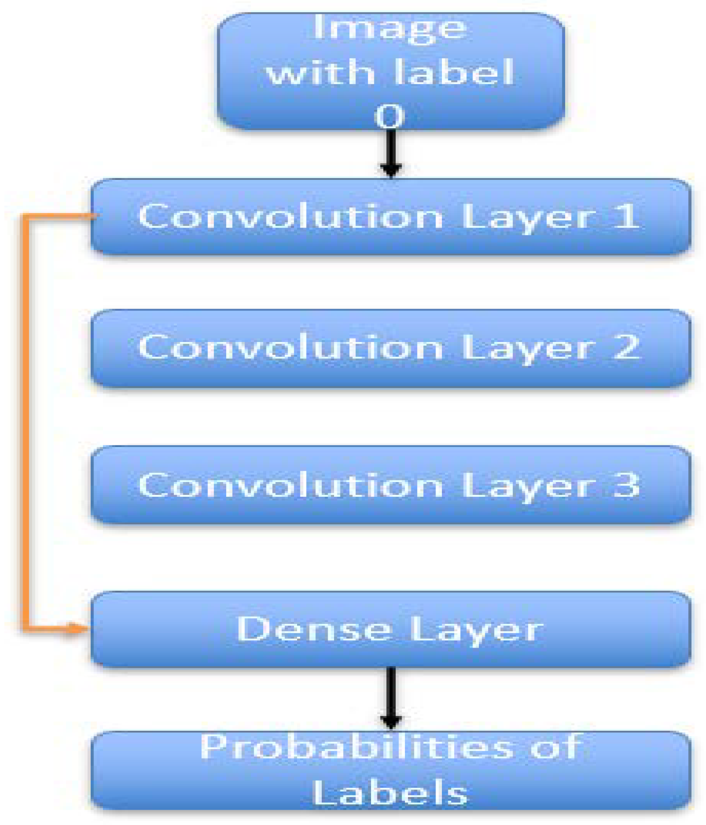
6] was used for training, validating, and testing a three-layered convolutional neural network (CNN 1) with one dense layer. It is important to note that there were no max pooling layers, and only the number of feature maps distinguished the three convolutional layers. For each of the three convolutional layers, the first ten feature maps were selected. For each of the ten chosen feature maps in each of the three convolutional layers, images which produced the ten strongest activations (highest mean absolute values) were selected. This meant that there were a hundred images chosen for each of three convolutional layers.
Figure 1.
CNN – 1 architecture.
Figure 1.
CNN – 1 architecture.
Images were assigned labels depending on convolutional layer at which they produced one of the ten strongest activations. In case of repetition, the higher label was chosen since that convolutional layer was significant in processing the image.
A convolutional neural network (CNN 2) was trained based on this training data to predict the convolutional layer at which the input image produced one of the strongest activations.
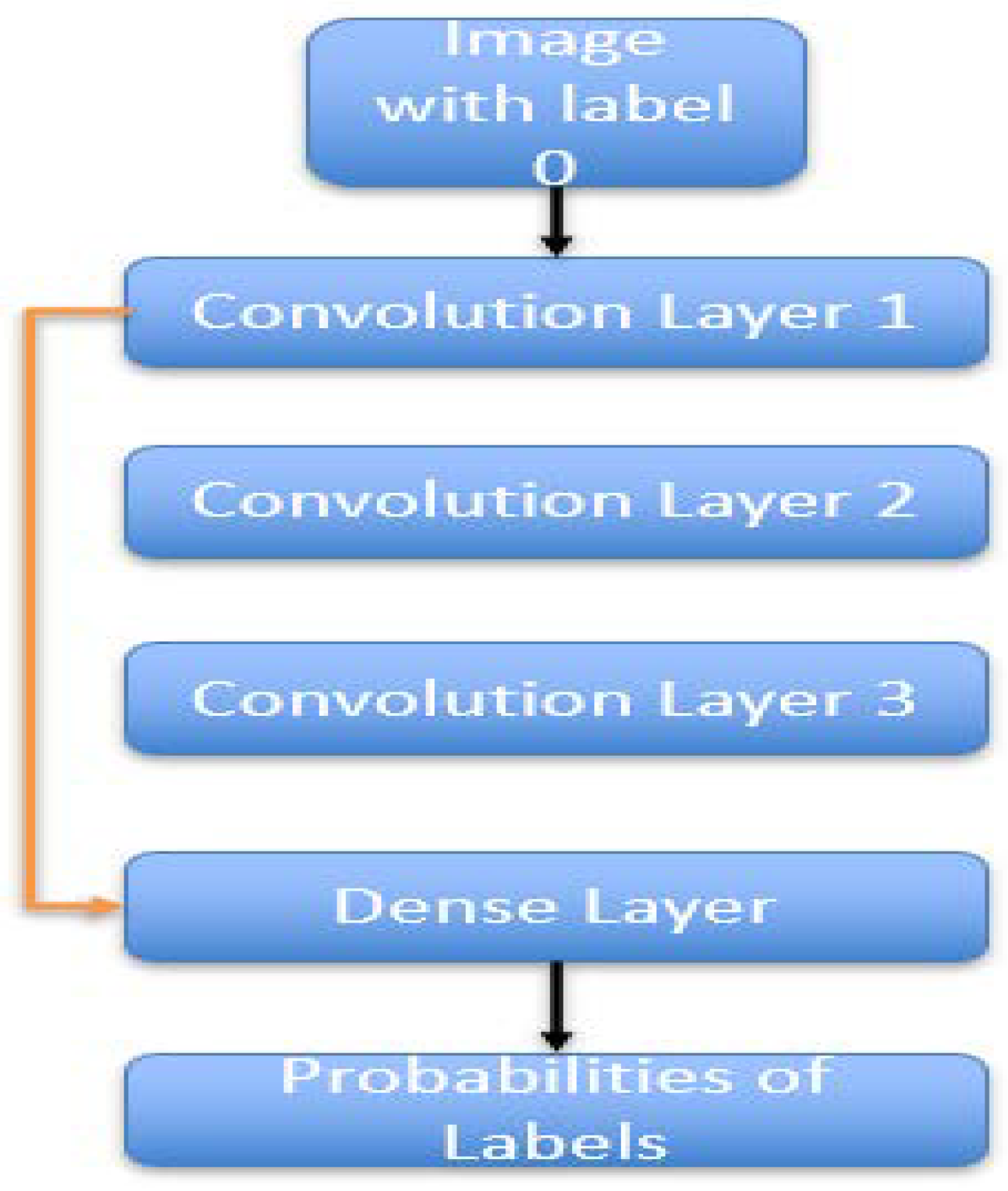
In the final step, the above-mentioned images and their corresponding labels were used to train another convolutional neural network (CNN 3). CNN 3 had the same architecture as CNN 1. It is to be noted that there were three unique labels 0, 1, 2 used. 0 was for the images which produced the strongest activations in the first convolutional layer. Similarly, labels 1 and 2 were for images that produced the strongest activations in the second and third convolutional layers respectively.
Figure 1.
CNN - 3 architecture.
Figure 1.
CNN - 3 architecture.
For the convolutional neural network (CNN 3), weights were initialized. For those images with label 0, the second and third convolutional layers were skipped in the forward pass. The first convolutional layer and the dense layer only were involved in the forward pass. Hence, weights corresponding to the first convolutional layer and the dense layer were updated. The weights corresponding to the second and third convolutional layers were left untouched. Similarly, for those images corresponding to label 1, weights corresponding to the third convolutional layer were left untouched, and other weights were updated after the forward pass skipping the third convolutional layer. For those images with label 2, no layer was skipped in the forward pass, and hence, all weights were updated.
For this to happen, i.e., skipping convolutional layers in forward pass, it had to be ensured that all the convolutional layers in CNN 3 had the same height and width.
The above-mentioned convolutional neural network was trained using RMSprop optimizer, ReLU activation function, sparse categorical cross entropy loss function and accuracy performance metric for 20 epochs. The above process was replicated for the CIFAR-100 dataset.
4. Results and Conclusion
CNN 2 was trained based on the training data obtained from training CNN 1 to predict the convolutional layer at which the input image produced one of the strongest activations. It had a test accuracy of 62 percent. Those results were used to train, validate, and test the convolutional neural network mentioned in the previous section (CNN 3). It had a test accuracy close to 100 percent, marginally higher than 98 percent when a convolutional neural network was used to train, validate, and test the MNIST dataset without any caveats (CNN 1). This result was validated using the CIFAR-100 dataset too.
5. Discussion
In this paper, we systematically reduced model complexity by eliminating irrelevant layers in CNN topologies. This improved model efficiency for computer vision modules. This work could be extended to more complex CNNs which include max-pooling layers, upsampling and downsampling operations, dilated convolutional layers, and residual layers [
7]. Furthermore, this methodology can be broadened to include other applications of computer vision like regression, semantic segmentation, image localization, and object detection.
Despite a relatively lower accuracy in label prediction using CNN 2, results from CNN 3 compare well to those from CNN 1 in the case of MNIST and CIFAR-100 datasets.
Author Contributions
Conceptualization, K.C.G. and S.B.D.; methodology, K.C.G.; software, K.C.G. and S.B.D.; validation, K.C.G., S.B.D., S.K. and K.N.; formal analysis, K.C.G. and S.B.D.; investigation, S.K. and K.N.; resources, S.K. and K.N.; data curation, K.C.G.; writing—original draft preparation, K.C.G. and S.B.D. ; writing—review and editing, K.C.G., S.B.D., S.K. and K.N.; visualization, K.C.G. and S.B.D.; supervision, K.N.; project administration, K.N.; funding acquisition, S.K. and K.N. All authors have read and agreed to the published version of the manuscript.
Funding
This research received no external funding.
Institutional Review Board Statement
Not Applicable.
Informed Consent Statement
Not Applicable.
Data Availability Statement
Conflicts of Interest
The authors declare no conflict of interest.
References
- Zeiler, M. D. , & Fergus, R. (2014). Visualizing and understanding convolutional networks. In Computer Vision–ECCV 2014: 13th European Conference, Zurich, Switzerland, -12, 2014, Proceedings, Part I 13 (pp. 818-833). Springer International Publishing. 6 September.
- Zeiler, M. D. , Krishnan, D., Taylor, G. W., & Fergus, R. (2010, June). Deconvolutional networks. In 2010 IEEE Computer Society Conference on computer vision and pattern recognition (pp. 2528-2535). IEEE.
- Krizhevsky, Alex, Ilya Sutskever, and Geoffrey E. Hinton. "Imagenet classification with deep convolutional neural networks." Communications of the ACM 60.6 (2017): 84-90.
- Simonyan, Karen, and Andrew Zisserman. "Very deep convolutional networks for large-scale image recognition. arXiv:1409.1556 (2014). [CrossRef]
- Szegedy, Christian, et al. "Going deeper with convolutions." Proceedings of the IEEE conference on computer vision and pattern recognition. 2015.
- LeCun, Y. (1998). The MNIST database of handwritten digits. Available online: http://yann. lecun.
- He, Kaiming, et al. "Deep residual learning for image recognition." Proceedings of the IEEE conference on computer vision and pattern recognition. 2016.
|
Disclaimer/Publisher’s Note: The statements, opinions and data contained in all publications are solely those of the individual author(s) and contributor(s) and not of MDPI and/or the editor(s). MDPI and/or the editor(s) disclaim responsibility for any injury to people or property resulting from any ideas, methods, instructions or products referred to in the content. |
© 2023 by the authors. Licensee MDPI, Basel, Switzerland. This article is an open access article distributed under the terms and conditions of the Creative Commons Attribution (CC BY) license (https://creativecommons.org/licenses/by/4.0/).


