3.1. Background of the ERT Model
The face alignment method presented in [
11] is based on the ERT model. In this method, the mean position of the landmarks stored in the trained model is gradually corrected in a number of cascade stages. In each cascade stage, a sparse representation of the input frame consisting of a few hundreds of reference pixels is used and a number of regression trees is successively visited. In each regression tree node, the gray level intensity of a pair of reference pixels is compared to decide the next node of the tree that has to be visited. When a leaf is reached, the corresponding correction factor is loaded from the trained model (different in each leaf of a tree) and this factor is used to correct the current landmark positions. In [
11], the focus was given on the training of the regression trees while in this paper we focus on the application of a trained model for the face shape alignment in successive video frames in runtime. A more formal definition of the training of the ERT model follows. Let
p be the number of face landmarks at a frame
frm, and
xi be a Cartesian coordinates pair. The shape
, drawn by these landmarks is defined as:
The training begins by initializing the shape
S to default positions. The exact position of the landmarks in the frame, which is currently examined, is refined by a sequence of
Tcs cascaded regressors. The current shape estimate in the regressor
t is denoted as
(t=1,.., T
cs). To continue with the next regressor, it is needed to estimate a correction factor
rt that depends on the frame
frm and the current estimate
. This correction factor
rt is added to
in order to update the shape of the face in the next regressor t+1:
. The
rt value is calculated based on the intensities of reference pixels that are defined relative to the current shape
. Every correction factor
rt is updated using a gradient tree boosting algorithm by adding the sum of square error loss. This training algorithm works with the group
. The training data is a set of
N images:
is the shape of any training frame with i
. The residual
in the regressor
rt+1 is estimated as [
11]:
The residuals are exploited by the gradient of the loss function and are calculated for all training samples. The shape estimation for the next regressor stage is performed as [
11]:
Then, for
K tests (k=1, …, K) in a regression tree and for
N training frames (i=1,…, N) in each test, the following formula is iterated:
In the k-th iteration, a regression tree is fitted to
rik using a weak regression function
gk, thus
fk is updated as follows [
11]:
where
lr<1 is the learning rate used to avoid overfitting. The final correction factor
rt of the t-regressor is equal to
fK.
In runtime, the algorithm begins by initializing the shape S to the mean landmark positions mined from the trained model. The exact position of the landmarks in the frame which is currently examined, is again refined by a sequence of Tcs cascaded regressors similarly to the training procedure.
The next node that should be selected in a regression tree of a specific cascade stage is estimated by comparing the difference in the gray level intensity between two reference pixels
p1 and
p2 with a threshold
Th. Different threshold
Th values are stored for every regression tree node in the trained model. The image is warped to match the mean shape of the face within a process called Similarity Transform (ST). If
q is a frame pixel and its neighboring landmark has index
kq, their distance
δxq is represented as
The pixel
q’ in the original frame
frm that corresponds to
q in the mean shape is estimated as [
11]:
The si and Ri are scale and rotation factors respectively, used in the ST to warp the shape and fit the face. The minimization of the mean square error, between the actual q’ value and the one estimated with eq. (6), is used to calculate the optimal values for si and Ri.
3.2. System Architecture and Operation
As noted the DSM module presented in this paper is based on the DEST video tracking application [
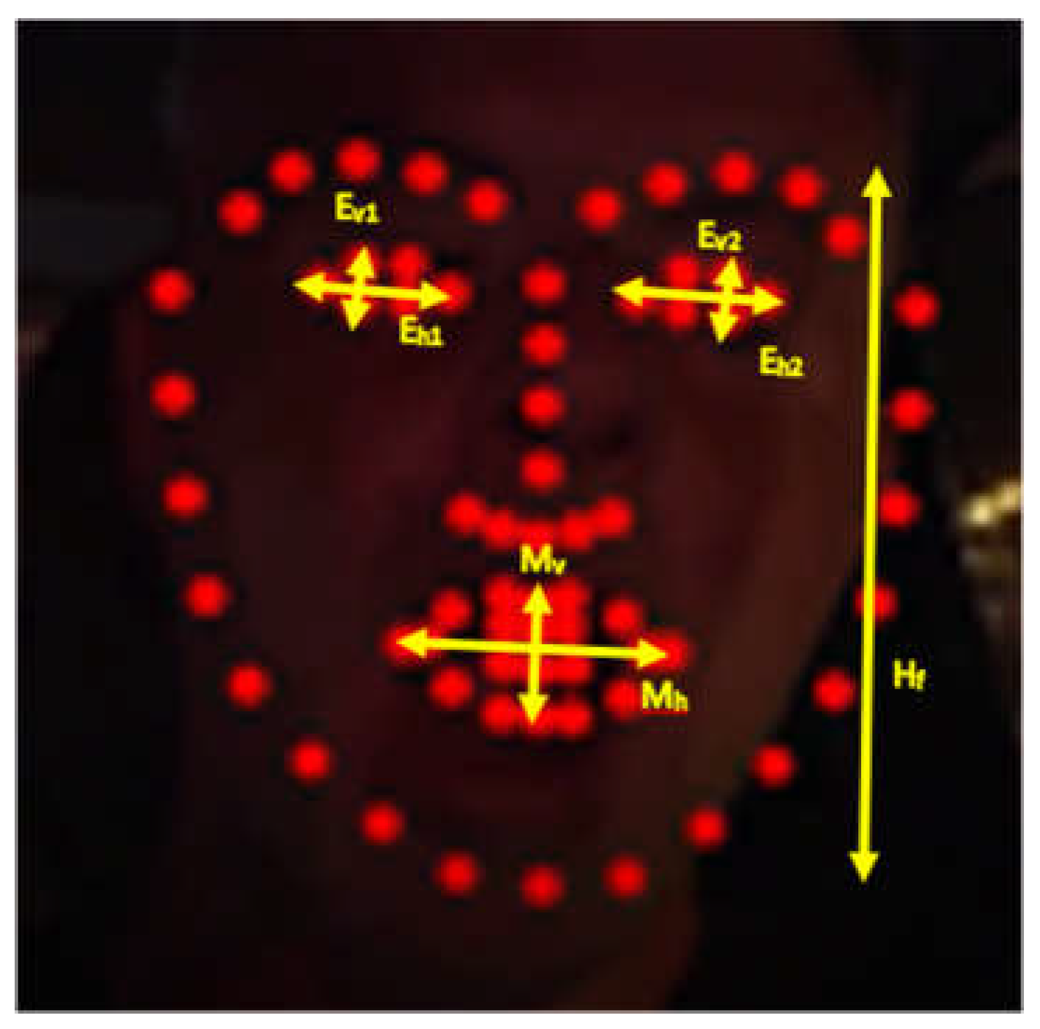
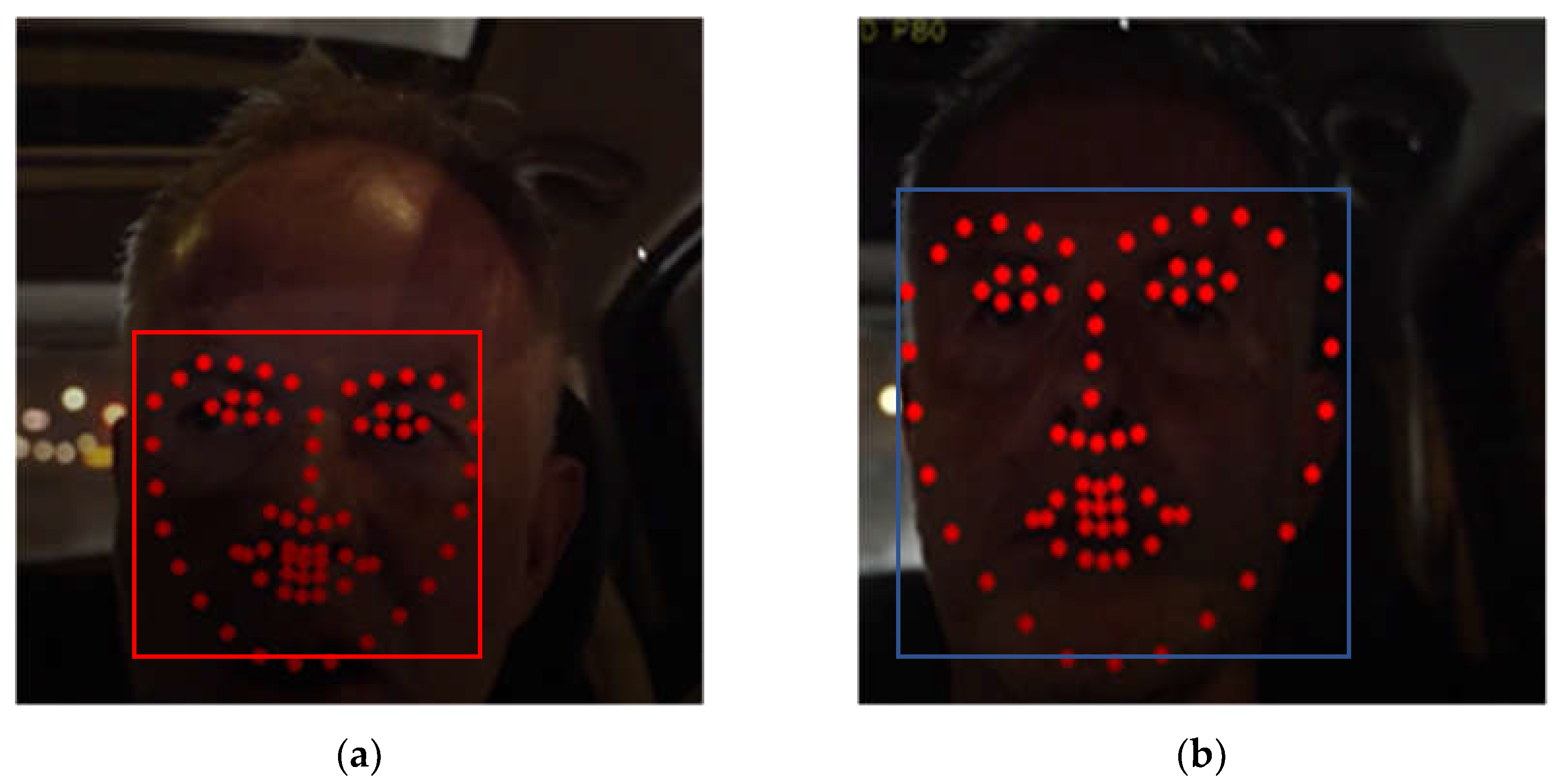
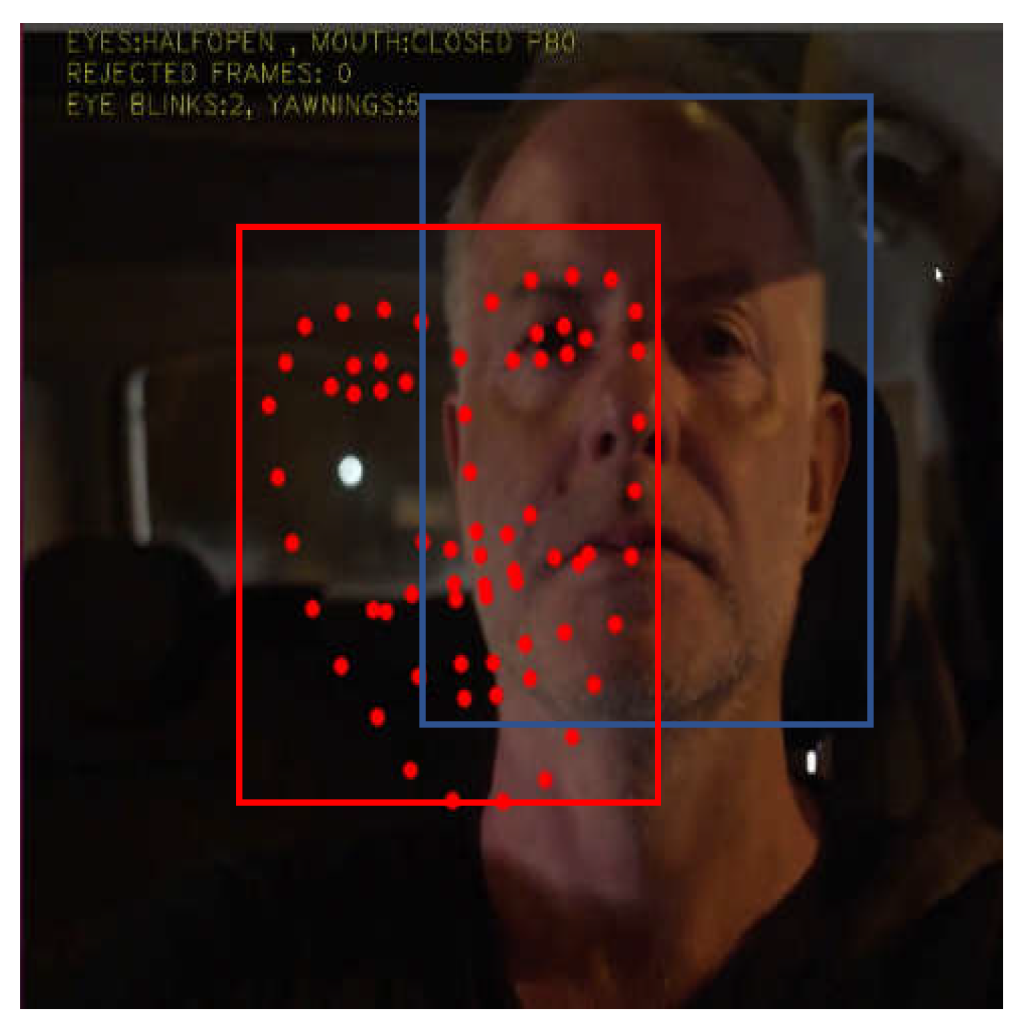
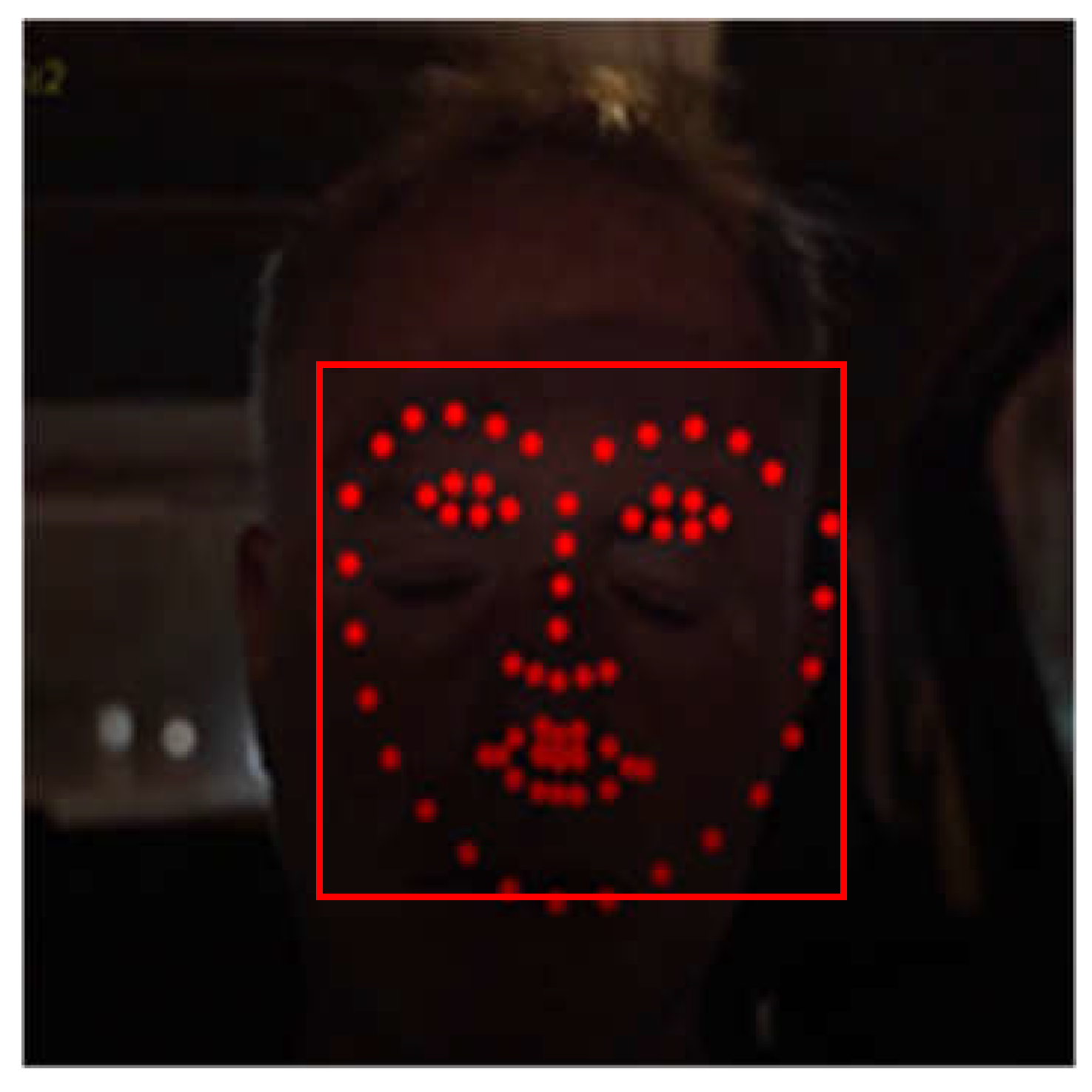
12] that matches landmarks on faces that are detected in frames from video or camera streams. Specifically, 68 facial landmarks are aligned as shown in
Figure 1. The Mouth Aspect Ratio (
MAR) of the vertical (
Mv) and the horizontal (
Mh) distance of specific mouth landmarks, can be used to detect yawning, if
MAR is higher than a threshold
TM for a number of successive frames:
Similarly, closed or sleepy eyes can be recognized if the average Eye Aspect Ratio (
EAR) of the eyes’ vertical (
Ev1, Ev2) and horizontal (
Eh1, Eh2) distances is lower than a threshold
TE for a period of time:
The parameter PERCLOS is the percentage of time that the eyes are closed and it is used to discriminate between a normal fast eye blink and an extended sleepy eye closure. Similarly, the percentage of time that MAR is higher than a threshold TM is used to distinguish a yawning from speech. In speech, the mouth is open and closed for shorter periods. For higher accuracy, more sophisticated ML techniques can also be employed to detect yawning or sleepy eye blinks instead of simply comparing with thresholds.
The dimensions of the face shape and the loss of focus can also be used to detect microsleeps or driver distraction. More specifically, during microsleeps the driver’s head is slowly leaning forward and then suddenly the driver wakes up raising his head. Therefore, a microsleep can be recognized if the face shape height
Hf (
Figure 1) is gradually decreased with a potential loss of focus (since no face is recognized by OpenCV when the head is down). Then, the face suddenly reappears to its previous normal position. Driver distraction can be recognized when the driver continuously talks or turns his head right and left without focusing ahead. Again, the shape dimensions, mouth pattern sequences, and loss of focus can be used to detect this situation. In this work we focus on yawning detection.
The video stream is defined during initialization and the frames are analyzed as follows. If face landmark alignment is required in a specific video frame, face detection takes place using the OpenCV library. For higher processing speed, a new face detection may be avoided in a few subsequent frames. In this case, the face is presumed to exist in an extended bounding box around the estimated landmarks from the previous frame. Landmark alignment is then applied in the bounding box returned by OpenCV using the DEST hierarchy of nested functions called: predict(). The Similarity Transform (ST) process, described in subsection 3.1, has to be practiced on the detected face bounding box to match its coordinates to those of the mean shape stored in the trained model. This model includes a set of regression trees in every cascade stage and the parameter values of each tree node are available from the training procedure.
As mentioned, the implementation of the ERT method [
11] in the open source DEST package [
12] was reconstructed to support acceleration of the computational intensive operations with reconfigurable hardware. The DEST implementation depends on the Eigen library that simplifies complicated matrix operations. The use of Eigen library calls in the original DEST source code protects from overflows, rounding errors, simplifies type conversions, etc. Eigen operators are overloaded to support various numeric types such as complex numbers, vectors, matrices, etc. The computational cost of these facilities is a reduction in the system performance. Furthermore, the Eigen classes are not suitable for hardware synthesis. To address this problem, the source code was simplified (re-written) replacing Eigen classes with ANSI C types that can be successfully ported to hardware using the Xilinx Vitis environment [
30]. Moreover, loops and large data copies were also optimized as will be explained in the next section.
To accelerate the DEST video tracking application in an efficient way, it was mandatory to profile the latency of the system components. To achieve this goal, the system was decomposed in potentially overlapping subsystems, estimating the bottlenecks and any resource limitations that occur if such a subsystem is implemented in hardware. The latency was profiled measuring the time from the beginning to the end of each subsystem operation. In this way, the computational intensive sub-functions were identified. Another factor that slows down the DEST video tracking application is the input/output argument transfer between the host and the subsystems implemented in hardware kernels. This is due to the limited FPGA Block Random Access Memory (BRAM) resources and the Advanced eXtensible Interface (AXI) bus port width. One major target of this work was to optimize big data transfer from the ARM cores to BRAMs with the lowest latency.
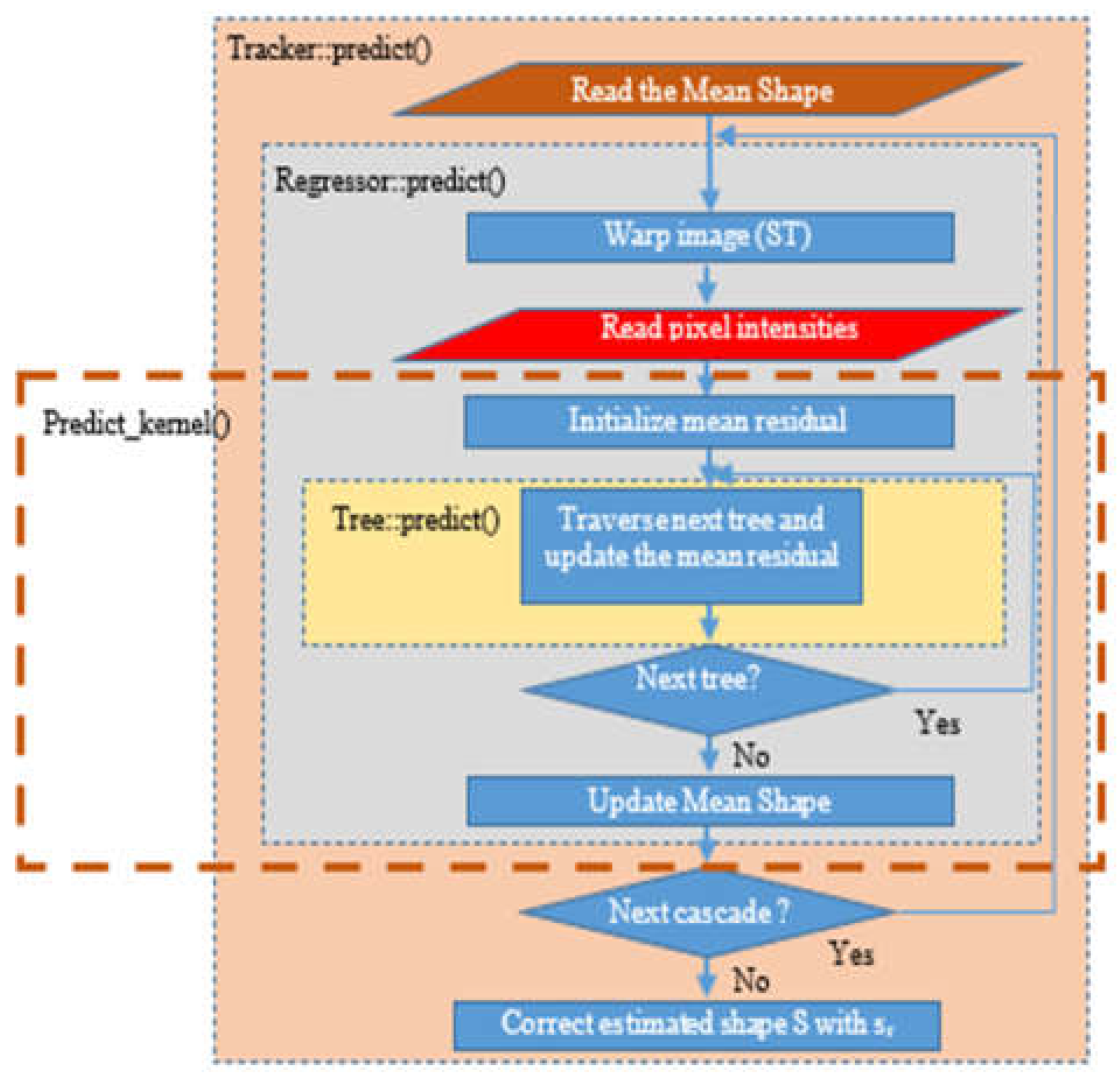
The profiling analysis indicated that the most computational intensive operation in the original DEST video tracking application is the
predict() function which incorporates three nested routines as shown in
Figure 2:
Tracker::predict(), Regressor::predict() and
Tree::predict().
Tracker::predict() is the top level function. Its input is the image frame
frm and the coordinates of the bounding box of the recognized face by OpenCV. This routine returns the final face landmark coordinates. The current shape estimate
S is initialized to the mean shape (that is stored in the trained model), at the beginning of the
Tracker::predict() routine. Then, the
Regressor::predict() is called inside
Tracker::predict(), once for every cascade stage. In our implementation, the default number of cascade stages is T
cs=10. The
Regressor::predict() accepts as input the image
frm, the face bounding box coordinates estimated by OpenCV and the current approximation of the shape estimate
S after applying the correction factor
f (see eq. (5)).
The Regressor::predict() calculates the residuals sr, that are used to optimize the estimate f in the Tracker::predict(). The Regressor::predict() routine employes ST to match the current landmark shape to the mean coordinates of the trained model. Then, the gray level intensities of a number of reference pixels are read from a sparse representation of the frm frame. The Tree::predict() function is invoked for all the stored Ntr binary regressor trees. In this implementation, the default number of regressor tress is Ntr=500. Every Tree::predict() computes a correction factor vector called mean residuals mr. A different mr vector is stored in the leaves of each regression tree. Each tree is traversed from the root to the leaves in the Tree::predict() routine, following a path defined dynamically: at each tree node, the difference in the gray level intensities of a pair of reference pixels that are indexed in the trained model, is compared to a threshold Th as already described in subsection 3.1. Either the right or left direction of the current node in the binary tree is selected, depending on the threshold Th that is also stored in the trained model. Each tree has depth equal to Td=5 and thus, nodes.
In the approach presented in this paper, a new Predict_kernel() routine was developed including operations from the Regressor::predict (and the nested Tree::predict). The Predict_kernel() routine has been implemented using ANSI C commands and a code structure that can be easily consumed by the HLS tool.
All the parameters of the trained model that were continuously accessed throughout the operation of the original DEST application are now loaded during initialization. All the model parameters are stored into buffers within the new predict_prepare() routine that is called when the system is powered up. More specifically, the number of the Ntr regression trees and their node values are read: the threshold Th, the mean residual mr, and the indices of the reference pixels that their intensity has to be compared with Th. Moreover, the LM=68 coordinates of the mean shape landmarks and the Nc reference pixel coordinates of the sparse image are also read from the trained model within predict_prepare().
The parameters that are not read once but have to be read again each time the Tracker::predict() is called, are the default mean shape estimate and the mean residuals. These values have to be re-initialized since their value is modified during the processing of each frame. Pointers to these arguments as well as to frame-specific information (image buffer, image dimensions, position of the detected face) are passed to the Predict_kernel() routine. The final landmark shape is returned by Predict_kernel() and its homogeneous coordinates are converted to the absolute coordinates in order to display the landmarks on the image frame under test.
The whole Regressor::predict() function was initially considered as a candidate for hardware implementation but soon it was abandoned. The main reason for not porting the whole Regressor::predict() routine in hardware is that it contains functions that do not reuse data and require a large number of resources. More specifically, it includes ST and the function that reads the reference pixel intensities. These two functions are quite complicated and thus, require a large number of resources. Moreover, their latency is relatively short since they do not have repetitive calculations. Finally, Regressor::predict() requires a large number (more than 20) of big argument buffers that would not fit to BRAM. Forcing the hardware kernel to access the values of these buffers from the common RAM that is accessed both form the processing and the Programmable Logic (PL) units of the FPGA, would cause a significant bottleneck.
For these reasons,
Predict_kernel() was defined as a candidate for hardware implementation with a subset of operations from the
Regressor::predict(). The
Predict_kernel() routine consists from the loop that visits the regression trees and it is called once for every cascade stage. The ST and the routine that reads the reference pixel intensities are left out of this routine (see
Figure 2). Its arguments are only the parameters that are stored in each regression tree node (five buffers). The specific steps of the
Predict_kernel() routine are presented in Algorithm 1. The buffer arguments are listed in line 1: the residuals
sr, the mean residuals (correction factors)
mr, the intensities of the reference pixels that will be compared in each node with the corresponding threshold
Th and the indices to the next regression tree node that has to be visited according to the results of the comparison with
Th. These indices of the tree nodes are stored in two vectors called
split1 and
split2.
The buffers that are transferred to BRAMs and their specific sizes in the default ERT model (M0) are: (a) the reference pixel intensities (size:
Nc floating point numbers, e.g., 600×32 bits), (b) the
split1 and
split2 buffers (
Ntr trees × (2
Td–1) nodes × short integer size, e.g., 500×31×16=15,552 ×16 bits for each one of
split1 and
split2), and (c) the
Th buffer (
Ntr trees × (2
Td–1) nodes × floating point size, e.g., 500×31×32bits). The mean residuals’ buffer (
mr) is too large (
Ntr trees × (2
Td–1) nodes × 136 landmark coordinates × floating point size, e.g., 500×31×136×32=15,552 ×32bits) to fit in a BRAM, therefore it has to be accessed from the common DRAM. The BRAMs are created and the corresponding arguments that will be store there are copied through a single or double, wide data port as will be explained in the next section, using optimized loops in steps 2 to 6 of Algorithm 1. Each argument is considered to consist of two data segments: the 1
st data segment stores parameters from the first N
tr/2 trees and the 2
nd data segment from the last N
tr/2 trees. If double data ports are used for each argument, the two data segments of each argument are processed in two parallel loops in step 7. If a single data port is employed for each argument, the two loops of step 7 will simply not be executed in parallel. The partial correction factors
sr1, sr2 are then added to the previous value of the overall correction factor
sr, which is returned to the caller of the
Predict_kernel() routine.
|
Algorithm 1. Predict_kernel() algorithm implemented as a hardware kernel. |
| Predict_kernel() |
Read arguments from the host (sr, split1, split2, Th, mr, reference pixel intensities) Create BRAM arrays for split1, split2, Th, and reference pixel intensities Loop to store pixel intensities Loop to store split1 (from a single or double, wide data port) Loop to store split2 (from a single or double, wide data port) Loop to store Th thresholds (from a single or double, wide data port) -
Parallelize the estimation of the correction factor to take advantage of double data ports:
- 7.a.
For every tree update the correction factor sr1 (1st data segment) - 7.b.
For every tree update the correction factor sr2 (2nd data segment)
Update the correction factor sr= sr +(sr1+sr2). Return sr to the host. |
3.3. Hardware Acceleration Methods
The employed hardware acceleration techniques are listed in
Table 1. Based on the system component profiling, the hardware implementation of initially the
Regressor::predict() function and then of the
Predict_kernel() was carried out using Xilinx Vitis High Level Synthesis (HLS) tool.
The most important optimization, concerned the efficient data buffering in order to reduce data transfer latency by more than 20ms from ARM core to the hardware kernel. The widest AXI bus data port that can be defined, is exploited to read concurrently the maximum range of data instead of only a single element during the argument transfer. Xilinx supports the technology to feed any time the kernel with Nb bits of the argument. More specifically, if an argument element requires an m-bit representation, it is feasible to transfer Nb/m elements in every clock cycle. For example, if bytes are transferred then the value of m is 8 while if integers or single precision floating point numbers are transferred then m=32. To store these data in parallel it is important to declare an array partition with multiple ports. This implementation requires a data type with arbitrary precision. The Xilinx ap_int<N> type provides the flexibility to slice the argument buffers into equal data pieces depending on the application requirements. For example, if it is assumed that 32 elements of 64 bits need to be stored in parallel, the kernel argument can be defined as ap_int<1024> and 16 elements can be read at once. Two clock cycles are only needed to read all the 32 elements. The next step is to declare an array of 64-bit elements with dimensions 16x2, which will be partitioned using the OpenCL ARRAY_PARTITION pragma in order to achieve maximum parallelization. With this technique any data conflict is avoided, and the data are read with the minimum possible latency.
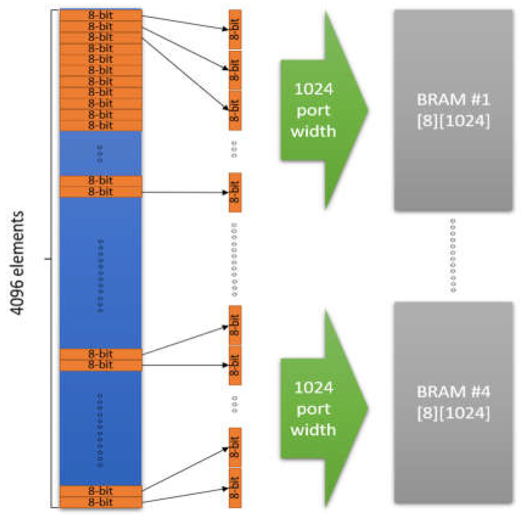
The OpenCL array partition operation can be optimized depending on the application. The type of the partition, the dimensions of the array that will be partitioned (all the array or a part of it) and the number of partitions that will be created can be defined with OpenCL. In this approach the most efficient way to partition the BRAM arrays was in block mode in order to achieve the maximum parallelization. The block factor that is used depends on how the memory is accessed for internal computations. The BRAM and AXI data port scheme employed in the developed DSM module is based on the example block diagram of
Figure 3. If an argument of 4096 bytes has to be transferred to 4 BRAMs in the hardware kernel, then four AXI ports of 1024-bits width can be used in parallel to transfer 128 bytes of the argument in each BRAM at one clock cycle. The transfer of the whole argument will be completed in just 4096/(128×4)=8 clock cycles. If a single 1024-bit AXI bus port was used to transfer the argument in a single BRAM of 4096 bytes then, 4096/128=32 clock cycles would be required. The fastest implementation of the
Predict_kernel() routine presented in this work, employs two AXI bus ports of 1024 bits in order to transfer each one of the
split1,
split2 and
Th thresholds arguments in a pair of independent BRAMs (i.e., six BRAMs are used in total to store these three arguments). An implementation with single ports per argument is also developed to compare the difference in the speed and the required resources. The ZynqMP Ultrascale+ FPGA does not provide enough resources to test more than two data ports of 1024-bit per argument.
As already described in the previous section, the sizes of split1 and split2 arguments (and the corresponding BRAMs) are 15,552 short integers of 16-bits and there are 15,552 threshold Th floating point values of 32-bits. If single wide ports of 1024-bits are used, then 1024/16=64 elements of split1 and split2 and 1024/32=32 elements of threshold values can be concurrently transferred in the three BRAMs of the hardware kernel. The time needed to transfer the split1, split2 and the thres arguments with single wide data ports, is 15,552/64=243 clock cycles and 15,552/32=486 clock cycles, respectively. If double ports are used for the split1, split2 and thres arguments, then the transfer of these arguments can be completed theoretically in half time. The BRAM of each argument will split in two components with equal size. In both cases (single and double data ports), the Nc reference pixel intensities (e.g., 600 floating point numbers) are also transferred in a BRAM through a wide port of 800 bits that allow the concurrent transfer of 800/32=25 values in 600/25=24 clock cycles. Due to the small size of this argument, it is not split in multiple data ports.
Xilinx provides coding techniques which force the synthesizer to implement an operation in hardware following specific rules. One of these coding techniques is the Resource pragma. This directive allows the use of specific resource types during implementation. More specifically, with this technique it was feasible to apply memory slicing using BRAMs for array partition instead of the Look Up Tables (LUTs) that the synthesizer uses by default. This is necessary since BRAMs with memory slicing show a lower access latency than LUTs. In this application, Dual Port BRAMs were employed to improve parallelization.
To store the data in the BRAMs and take advantage of the parallelization, for-loops were used to store several elements of data in parallel in each iteration. To reduce latency during this procedure, the Pipeline pragma was used. This directive reduces the latency between consecutive Read or Write commands whenever possible. Pipeline is a technique that is used frequently at parallelization and in our approach, it was employed throughout Algorithm 1 (steps 2-8).
Another important acceleration technique was the selection of the appropriate communication protocol between the kernel and the host. It was important to calculate the size of the data that will be transferred from the host to the kernel and in the opposite direction in order to select the appropriate communication protocol. In this approach, an AXI master-slave interface was selected through the Interface directive. There is a set of optional and mandatory settings giving the flexibility to choose the mode of connection, the depth of the First-In-First-Out (FIFO) buffer that will be used during synthesis and implementation phase, the address offset etc. A different AXI-Lite interface was used for each argument of the hardware kernel. The FIFO depth varies depending on the size of the data that will be transferred through the AXI interface.
Another hardware acceleration technique provided by OpenCL is the for-loop unrolling technique. If there are not any dependences between the operations of the consecutive iterations, then unrolling a loop permits the execution of the operations of successive iterations in parallel. Of course, if a loop is fully unrolled all its identical operations are implemented with difference hardware circuits consuming a large number of resources. As an example, if we focus on the loop of 136 iterations that update the 68 pairs of face shape coordinates in step 8 of Algorithm 1, there is no dependence between these iterations. In the case of full for-loop unroll, all the 136 additions of double precision floating point numbers could be executed independently in one clock cycle, instead of a single addition per clock cycle. This technique is flexible since a partial loop unroll can be applied to make a tradeoff between resource allocation and speed. For example, in step 8 of Algorithm 1, an unroll factor of 8 is used i.e., 8 double precision additions are performed in parallel in each clock cycle and 136/8=17 clock periods are needed to complete the whole step 8 instead of 136 clock periods that would be required if no loop unrolling was employed. Loop unrolling was also used for partial for-loop unrolling in step 7.
Some for-loops in the original DEST code were difficult to be unrolled in an efficient way. The original DEST code was reconstructed in this case to achieve a better hardware acceleration. More specifically, the for-loop that traverses the regression trees in step 7 of Algorithm 1 was split manually in 2 independent but computationally equal loops (in steps 7a and 7b of Algorithm 1) that read their split1, split2 and Th threshold arguments from the pairs of the BRAMs where these arguments were stored in steps 4-6 of Algorithm 1. In this way, the Vitis hardware synthesis recognizes these 2 sections as independent and implements them in parallel. For instance, instead of running a for-loop that traverses 500 regression trees, two for-loops of 250 iterations are defined that are executed in parallel. This method can be extended to more AXI-bus ports and BRAMs as long as the FPGA resources can support the resulting number of ports.
