Heat Wave Magnitude Projection in the Middle Awash Basin Under Coupled Model Intercomparison Project the 6th Phase (CMIP6)

Preprint

Article

Heat Wave Magnitude Projection in the Middle Awash Basin Under Coupled Model Intercomparison Project the 6th Phase (CMIP6)

Altmetrics

Downloads

146

Views

Comments

Supplementary Material

supplementary.csv (3.87KB )

Tadele Badebo Badacho^*

This version is not peer-reviewed

This preprints belongs to the Topic

Applications of Geodesy in Meteorological, Hydrological and Climatic Environments

Submitted:

30 May 2023

Posted:

08 June 2023

You are already at the latest version

Alerts

Abstract

Globally, the intensity and irregularity of weather and climate extremes are increasing due to climate change. In Ethiopia, the occurrence of extreme events has been increasing, reporting severe impacts on environment which led to losses of lives and livelihood of societies. In this study, Heat Wave Magnitude Index daily (HWMId) was used to analysis heat wave magnitude in the Middle Awash Basin of Ethiopia. Gauge data obtained from Ethiopian Meteorological Institution (EMI) for 1981-2022 period and the future projection was taken from Coupled Model Intercomparison Project Phase 6 (CMIP6) under two socioeconomic pathways (SSP 2 and SSP 5) scenarios. The findings clearly showed that the area aggregated annual temperature anomaly increasing each year, 2015 was one of the warmest year on record with an anomaly of +1.8 °C. Severe to extreme heat wave recorded particularly during the last 10 years. For the future projection, under SSP 2-4.5 forcing scenario, the annual average air temperature projected to be warmer, which increasing 1.7 ℃ to 1.8 ℃ during mid-century and 2.3 ℃ to 2.4 ℃ end of century. Meanwhile, for SSP 5-8.5 forcing, the projection indicated an increment of 2.2 ℃ to 2.5 ℃ under mid-century and 4.4 ℃ to 4.8 ℃ end of century. Concerning the severity of heat wave, extreme to very extreme heat wave projected under SSP 2-4.5 forcing scenario and supper extreme heat wave projected under SSP 5-8.5 forcing scenario, respectively. The increase in extreme events may have a negative impact on health, water availability and food security. Therefore, the result of this study are essential for making wise decisions and for developing suitable strategies for climate change adaptation and mitigation that could minimize the risk of unusually extreme weather events.

Keywords:

Subject: Environmental and Earth Sciences - Atmospheric Science and Meteorology

1. Introduction

The earth's surface and troposphere are substantially warmed by a rise in the concentration of greenhouse gases (GHG) in the atmosphere reported by Intergovernmental Panel on Climate Change (IPCC) and World Meteorological Organization (WMO). As a result, the average global temperature in 2021 was increased by 1.11 +0.13 °C above the pre-industrial (1850-1900) levels. 2021 was the seventh consecutive year (2015-2021), making 2015 the warmest year in the period of instrumental data (IPCC a, 2014, Russo et al., 2015, Hansen et al., 2016, WMO, 2022).

The future projection shows that a global average temperature expected to increase in the range of 1.5 °C-4.8 °C above pre-industrial levels. The Sixth Assessment Report (AR6) of IPCC projection indicated that in the coming decades climate change increase in all regions for 1.5 °C of global warming, there would be increasing extreme events like heat waves, longer warm seasons, droughts and floods. Moreover, the report shows at 2 °C of global warming, heat extremes would more often reach critical tolerance thresholds for agriculture and the health (IPCC a, 2021).

A changing climate may lead to changes in the frequency, intensity, duration and timing of extreme weather and climate phenomena which result in unprecedented climate related disasters. The risks of exposure and vulnerability were not minimized, extreme weather and climatic events severely impact on nature and human systems. Despite of efforts to reduce the risks, human-induced climate change is distracting the environment in widespread way and affecting the lives and livelihood of millions of people, according to the IPCC's assessment report six (AR6) on adaptation and vulnerability (IPCC, 2022). According to Center for Research on the Epidemiology of Disasters (CRED) report, climate change, climate variability and extreme weather events stance a threat to the eradication of extreme poverty in developing nation and should serve as a spur to accelerate efforts not only to reduce Green House Gas (GHG) emissions but also to challenge other underlying risk drivers such as vulnerable livelihoods, environmental degradation and gaps in early warnings systems (CRED, 2015).

The objective of this study is to investigate changing pattern of heat waves in 1981-2022 and to project future heat wave occurrence in 2041-2070 and 2071-2100 period over Lower Awash Basin, Ethiopia, using Heat Wave Magnitude Index daily (HWMId). The HWMId is a dimensionless magnitude that is designed to take into account both heat wave duration and magnitude, which is recently introduced by (Russo et al., 2015). The maximum magnitude of heat wave in a year is measured by HWMId, where a heat wave is defined as a period of three consecutive days where the maximum temperature exceeds the daily threshold for the reference period. The threshold is the 90th percentile of daily maxima, centered on a 31-day window (Russo et al., 2015).

In this study, the latest Global Climate Models (GCMs) developed under the 6^th phase of Couple Model Intercomparison Project (i.e., CMIP6) are used for the heat wave projection and simulation. CMIP6 models lead previous generations with improved spatial resolutions, enhanced parameters of the cloud microphysics process, and other earth system processes and components such as biogeochemical cycles and ice sheets. Furthermore, CMIP6 uses socioeconomic pathways (SSPs) which are considered as more realistic future scenarios (Neill et al., 2018). The SSPs are based on five narratives, describing alternative socioeconomic developments, including sustainable development, regional rivalry, inequality, fossil-fueled development, and middle-of-the road development (Riahi et al., 2016). Compared to previous scenarios i.e., Representative Concentration Pathways (RCP), SSPs offer a broader view of a “business as usual” world without future climate policy, with global warming in 2100 ranging from a low of 3.1 °C to a high of 5.1 °C above pre-industrial levels (Neill et al., 2018).

2. Materials and Methodology

2.1. Study Area Description

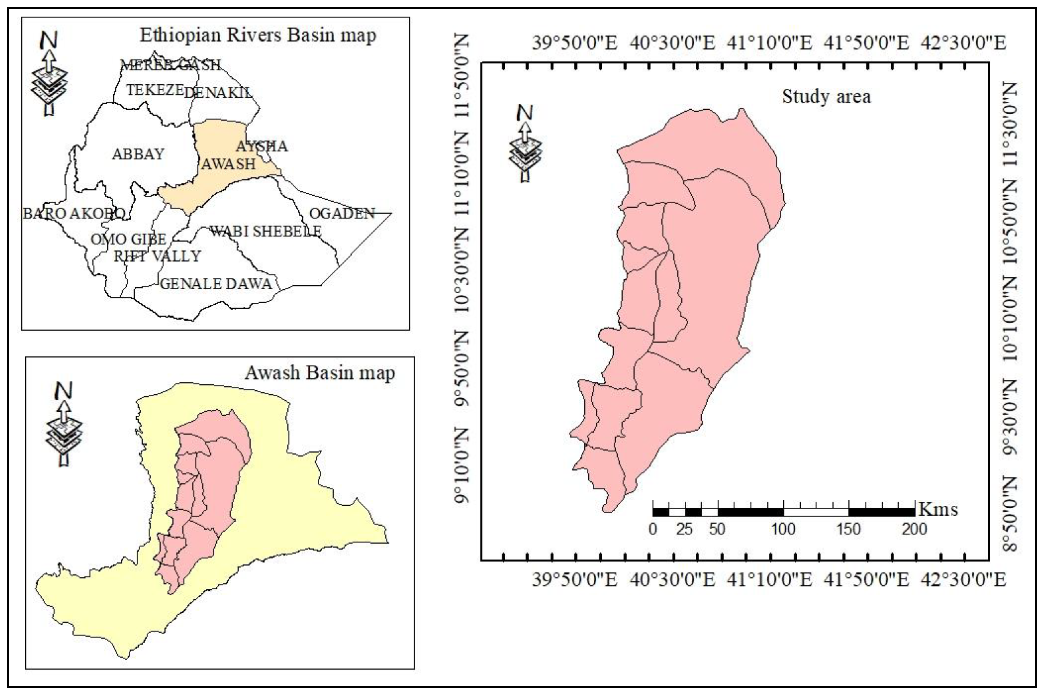
The study was conducted in the Middle Awash Basin (MAB) of Ethiopia which is located between latitude of 8° 83' and 11° 60' North and between longitude of 39° 79' and 41° 00' East (Figure 1).

2.2. Data Sources and Types

2.2.1. Observation Dataset

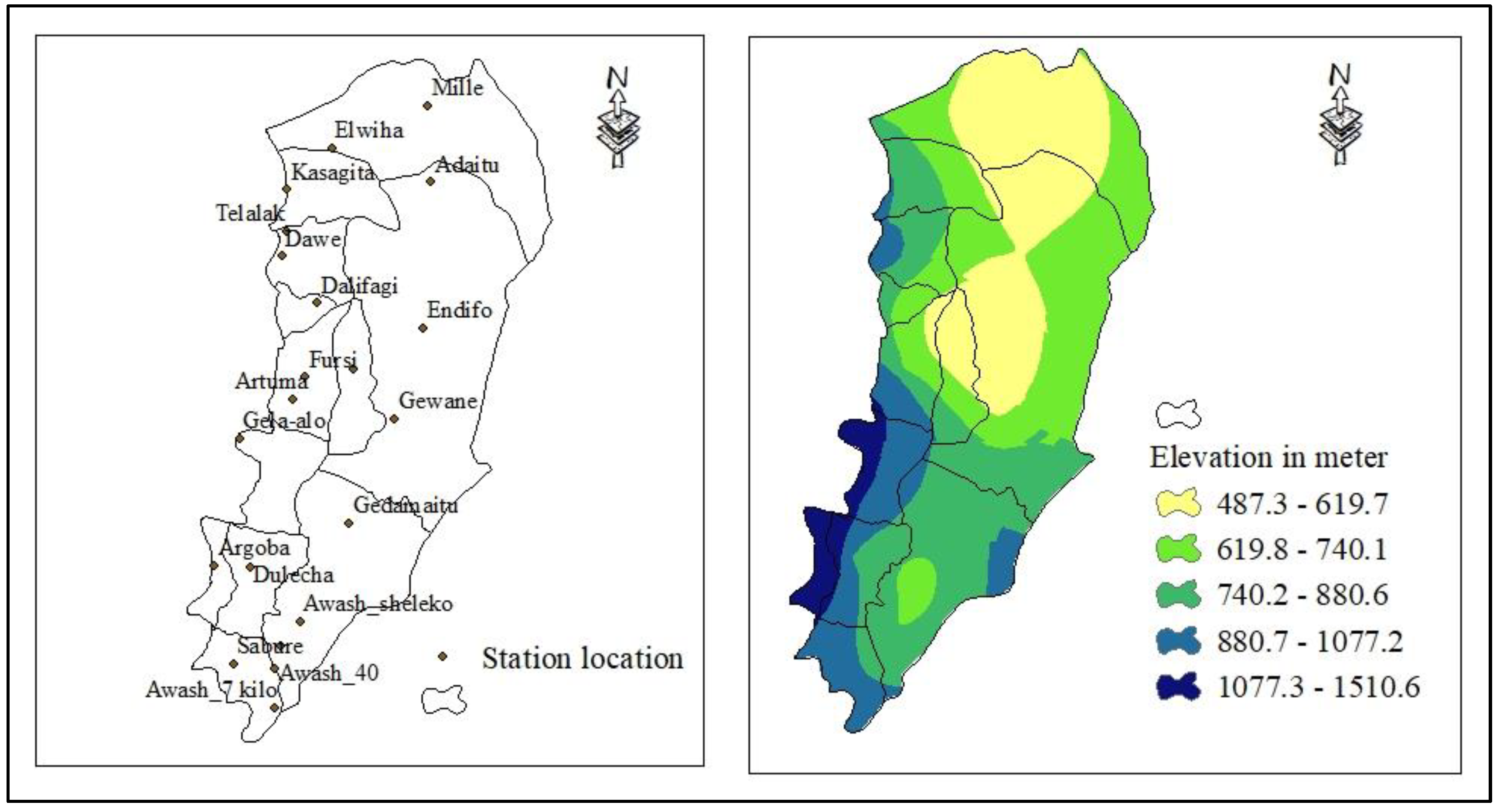
In the research area, there are 21 conventional stations according to a report from the National Meteorological Agency (NMA) of Ethiopia. Daily maximum and minimum temperature was collected from a total of 21 weather stations for 1981-2022 period which are located in Afar regional state and administrated by Ethiopian Meteorological Institution (EMI) (Figure 1).

Figure 2. Station distribution (left side) and elevation map (right side) of study area.

2.2.2. AgERA5 Dataset

Since many of the stations have short records and data gaps, the European Center for Medium-Range Weather Forecast's (ECMWF) Agrometeorological indicators 5^th Generation Atmospheric Reanalysis (AgERA5) dataset is downloaded 1. The AgERA5 dataset is stored in the NetCDF-4 (Network Common Data Form, version 4) file format and extracted using python programming with latitude and longitude of each stations. These dataset has a resolution of 10 by 10 km and here utilized to fill the gaps in observation. Before filling the gap in observation, the quality of AgERA5 was tested by Pearson correlation and corrected using Linear Scaling (LS) bias correction approach. The scaling approach mainly includes linear approaches that adjust the climatic factors based on the differences between observed and simulated dataset (Zollo et al., 2014).

2.2.3. CMIP6 Dataset

The models used in this study comes from five climate models from the r1i1p1f1 variant listed in Table 1. The models are implemented by the European Commission, ECMWF which is downloaded from CMIP6 achieve 2 on March 14 2023. CMIP6 netCDF file metadata includes the variant-id global attribute which has the format r1i1p1f1, where the numbers are indices for particular configuration of: r indicates realization (i.e. ensemble member), i represents initialization method, p represents physics and f represents forcing, respectively. CMIP6 data underpins the IPCC 6^th assessment report and spans for simulations of present climate (1981-2014) and future projection (2015-2100) period. The data are produced by the participating institutes of the CMIP6 project described in (Table 1).

2.2.4. Reference Datasets

According to World Climate Data Program (WCDP) and World Meteorological Organization guideline, an acceptable percentage of missing data in a data set to compute normal or average for a given month, data should be available for at least 80% of the years in the averaging period (WCDP, 1986, WMO, 2006). Therefore, Gewane station was selected as Reference Climatological Stations (RCSs) due to the longer length of data record. The available data was in the range of 81%-83%, respectively. These station dataset was used to evaluate AgERA5 performance against observation. The CMIP6 dataset is stored in the NetCDF-4 file format, therefore, extracted using python programming with latitude and longitude of the study area. The Python 3 (version 3.9) was download 3 and here used to fill missing data in observation, bias correction and extract NetCDF-4 file into excel format. Since the climate data was a point observation from 21 sites for 1981-2022 period, the 21 site dataset were aggregated and taken as an area average for the entire study area.

2.3. Methodology

2.3.1. Heatwave Magnitude Index daily (HWMId)

The HWMId was an improvement of the HWMI proposed by (Russo et al., 2014), which is defined as the maximum magnitude of the heatwaves in a year. Heatwave is defined as a period of three consecutive days with maximum temperature (Tmax) above the daily threshold for a reference period. The threshold is defined as the 90^th percentile of daily maximum temperature, centered on 31-day window. Hence, for a given day d, the threshold is the 90^th percentile of the set of data

A_{d}

defined by:

A_{d} = U_{y} {\in Y_{r e f} U_{i} \in {W_{d}}^{- 15, 15} T}_{m a x, y, i,}

(1)

where

\cup

denotes the union of sets,

Y_{r e f}

represents the years within reference period,

{W_{d}}^{- 15, 15}

is the 31-day window entered at day

d

and

T_{\max, y, i,}

is the daily maximum temperature of the

d a y i

in year

y

. HWMId magnitude is a sum of the magnitude of the consecutive days composing a heatwave (Russo et al., 2015), with daily magnitude

M_{d}

calculated as follow:

M_{d} (T_{d}) = \{\begin{matrix} \frac{T_{d} - T_{30 y 25 p}}{T_{30 y 75 p} - T_{30 y p}} i f T_{d} > T_{30 y 25 p} \\ 0 i f T_{d} \leq T_{30 y 25 p} \end{matrix}

(2)

where

T_{d}

being the maximum daily temperature on day d of the heatwave,

T_{30 y 25 p}

and

T_{30 y 75 p}

are the 25^th and 75^th percentile values, respectively, of the time series composed of 30 year annual maximum temperature within the reference period 1981-2010.

2.3.2. Cumulative Density Function Estimation

The kernel density estimator (KDE) was used to estimate the empirical probability distribution function (EPDF) and the associated empirical cumulative density function (ECDF) based on the annual maxima of the sub-heatwave unscaled magnitudes (Silverman, 2018). The general kernel density estimator for f is as follows: Given independent and identically distributed annual maxima of sub-heat wave unscaled magnitudes,

T_{1}

T_{2}

….

T_{N}

, with the common probability density function f(T), where N is the number of years:

\hat{f_{h}} (T) = \frac{1}{N} \sum_{i = 1}^{N} K (T - T_{i}, h)

(3)

T is the unscaled sub-heat wave magnitude, K is the kernel function, and h is the bandwidth smoothing value. Detailed evaluations of the kernel smoothing technique may be found in (Silverman, 2018). The Gaussian function is computed using the following kernel function, K:

K (X, σ) = \frac{1}{σ \sqrt{2 π}} e^{- \frac{x^{2}}{2 σ^{2}}}

(4)

By using the method of (Sheather & Jones, 1991), h is calculated, and the value of ECDF are obtained by integrating the

\hat{f_{h}} (T)

as follows:

E C D F (T) = \frac{1}{N} \sum_{i = 1}^{N} K \int_{- \infty}^{T} (T - T_{i}, h) d T

(5)

A descriptive classification of heat wave events based on the HWMId values was proposed by Russo et al., (2014), and it was presented in (Table 2).

2.3.3. Climate Model Performance

In this study, two performance measures, namely Pearson correlation coefficient (r) and coefficient of variation (CV), were utilized to examine the performance of GCMs. Pearson correlation coefficient is a number between -1 and +1 which measures the relationship of strength between two continuous variables (Pearson, 1920). The CV is a statistical measure that shows the variation of data point from the mean which is the ratio of standard deviation to the mean (Equation (6)), and used to evaluate the dispersion or the degree of variation from one data point to another. CV is used to apply in solving quality control, reliability problems and comparison of relative dispersion. High values of this statistics result from high variability in quality (Irvin, 1970).

C V = \frac{σ}{μ}

(6)

where

σ

and

μ

denote standard deviation and mean of dataset, respectively.

Comparing the performance of each selected GCMs and their average with observation, the average of selected models has lower CV and higher r than each GCMs for the reference period (Figure 3). The Pearson’s correlation coefficient (r) showed a positive linear relationship between area averaged observation and selected GCMs with correlation coefficient in the range of 0.39 to 0.78). MPI-ESM1-2-LR has higher r value than other selected GCMs models. EC-Earth3-CC and MRI-ESM2-0 have lower CV, while MPI-ESM1-2-LR, INM-CM5-0 and GFDL-ESM4 have higher CV when compared to observation. In general, the area averaged ensemble of GCMs was showed good performance, lower CV and higher correlation coefficient (Figure 3).

3. Results and Discussion

3.1. Heatwave Magnitude

For this study, daily near surface air temperature was extracted from five GCMs listed in Table 2-1. The observed dataset was area average, and similarly future projection of heat wave was an average of all selected climate models. The model dataset was bias corrected and checked their skills whether or not simulating local climate of the study area.

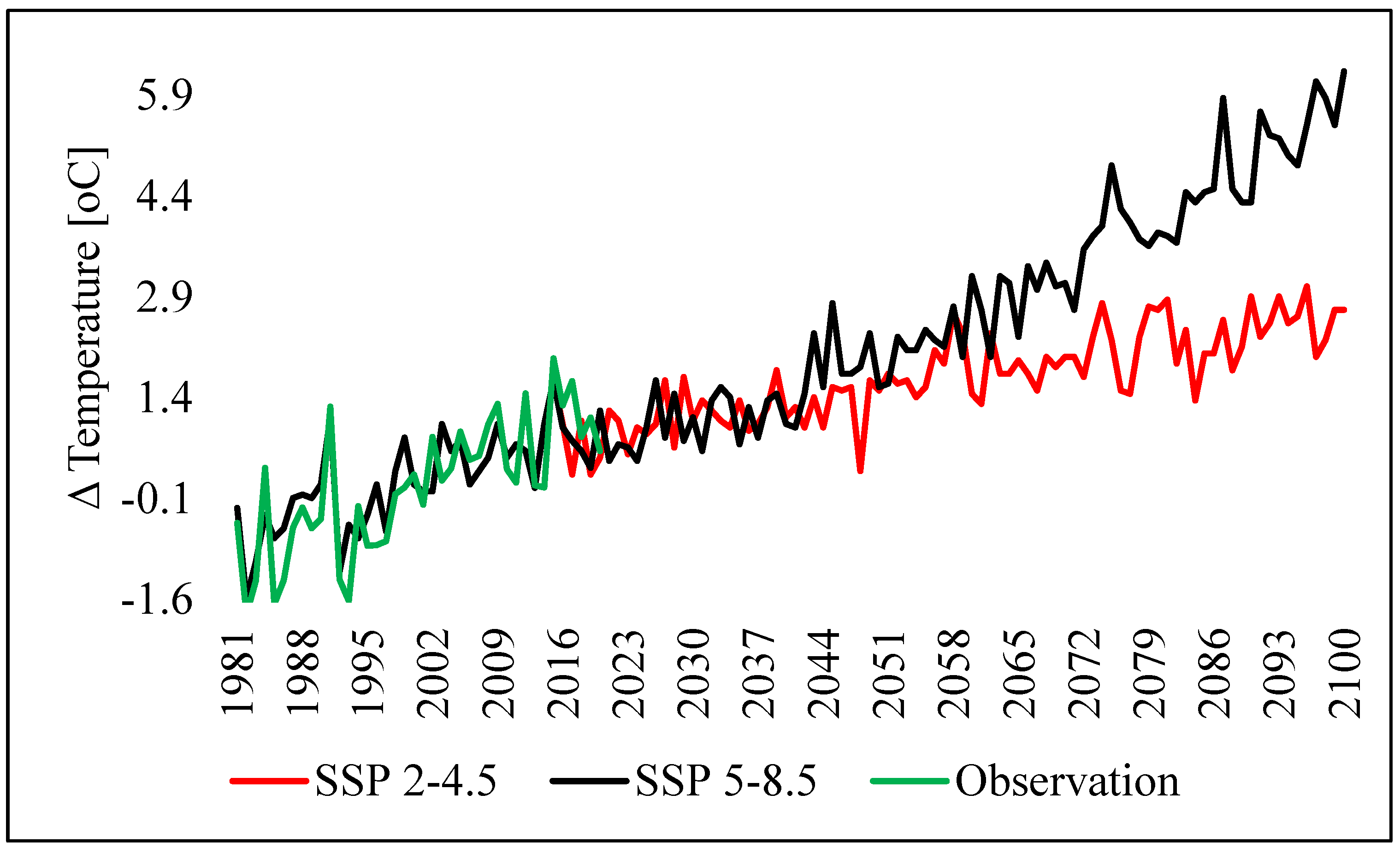
The result showed that the area averaged annual temperature anomalies have increased over the study area at an average rate of +0.7, with 2015 was one of the warmest years on record with an anomaly of +1.8 °C (Figure 4). The projected change in annual temperature showed that under SSP 2-4.5 forcing scenario, the annual average air temperature projected to be warmer, which increasing 1.7 ℃ to 1.8 ℃ during mid-century and 2.3 ℃ to 2.4 ℃ end of century. Meanwhile, for SSP 5-8.5 forcing, the projection indicated an increment of 2.2 ℃ to 2.5 ℃ under mid-century and 4.4 ℃ to 4.8 ℃ end of century (Figure 4).

3.2. Heat Wave Magnitude Index daily (HWMId)

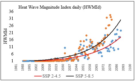
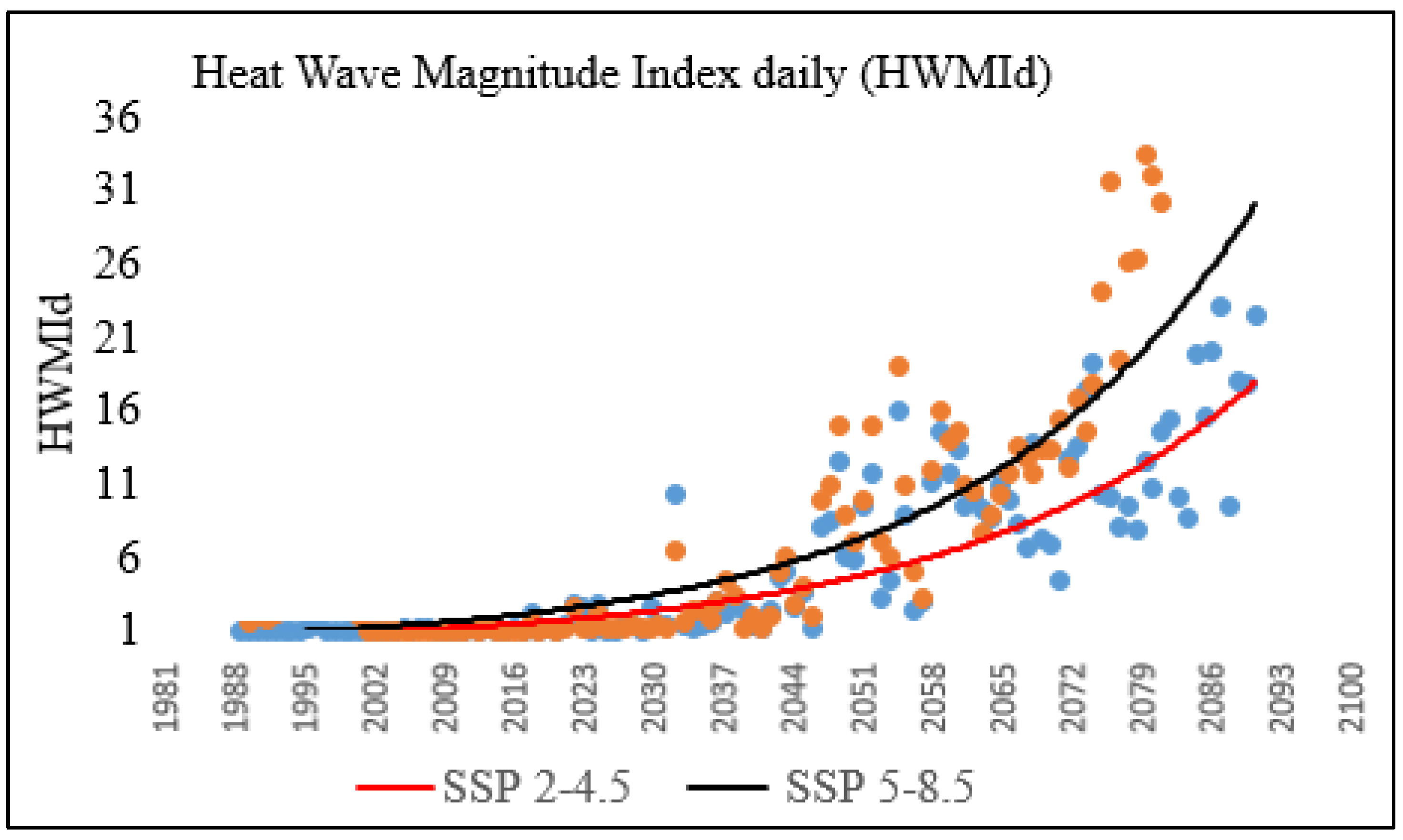
The average HWMId under SSP 2-4.5 and SSP 5-8.5 scenarios for the study area was presented in Figure 5. Each data point i.e., blue dot for SSP 2-4.5 and orange dot for SSP 5-8.5 scenarios represents an individual year, while the annual ensemble average values (smoothed) were shown by red curve for SSP 2-4.5 and black curve for SSP 5-8.5 scenarios, respectively. From the beginning of the simulations until approximately the year 2030, normal and moderate heatwave conditions prevail on average. This is expected since the criteria for identifying heatwave days were based on the recent past reference period. The models, on average suggest a transition to severe and extreme events by 2031-2051. For the following decades and towards the end of the 21^st century, thermal conditions were projected to become particularly harsh, as the so-far unobserved and thus unprecedented super-extreme and ultra-extreme events were projected to become common under the business-as usual (Figure 5).

The results, which were generally consistent with previous studies, showed that the climate change was driving an increase in heat wave across the global, relative to the long-term average. The year 2015 was the hottest on record in a long-term trend of increasing surface temperatures worldwide ( Russo et al., 2015, Hansen et al., 2016). The finding also agreed with similar work in Ethiopia that the past and future climate projections increasing under CMIP6-SSPs scenarios (Alaminie et al., 2021, Gebresellase, 2022, Balcha et al., 2022). Balcha et al., (2022) also noted that the average annual maximum temperature projected to increase 1.6 ^o C for SSP2-4.5 scenario, 2.0 ^o C for SSP5-8.5 scenario at mid-century and 2.0 ^o C for SSP2-4.5 scenario and 3.0 ^o C for SSP5-8.5 scenario at end of century.

4. Conclusions

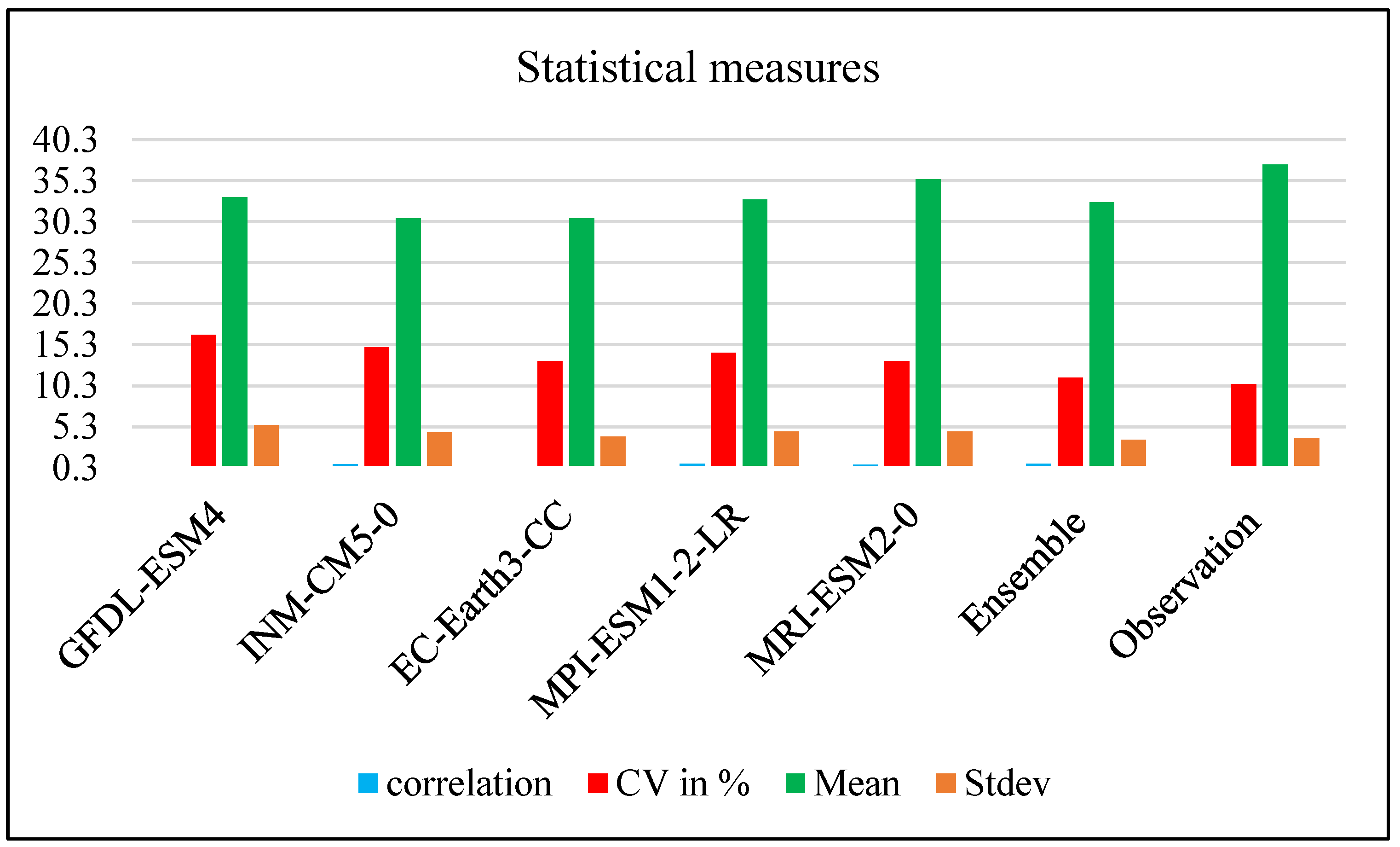
This study investigated present heat wave magnitude and projected future heat wave occurrence in Middle Awash Basin using area average observed data and five GCMs under SSP 2-4.5 and SSP 5-8.5 scenarios. Initially, AgERA5 data was downloaded and bias corrected, and filled the gap in observation. The performance of the GCMs in reproducing observed historical heat wave magnitudes was evaluated by comparing the area averaged observation data using two statistical measures, Pearson Correlation and Coefficient of Variation.

The result showed that the area aggregated heat wave increasing each year, 2015 was one of the warmest year on record with an anomaly of +1.8 °C. Severe to extreme heat wave recorded particularly during the last 10 years. The finding also clearly indicated that extreme to very extreme heat wave projected under SSP 2-4.5 forcing scenario and supper extreme heat wave projected under SSP 5-8.5 forcing scenario, respectively.

Climate change and extreme weather events pose a threat to the eradication of extreme poverty, and also challenge other underlying risk drivers such as vulnerable livelihoods, environmental degradation and gaps in early warning system. Therefore, the result of this study are essential for making wise decisions and for developing suitable strategies for climate change adaptation and mitigation that could minimize the risk of unusually extreme weather events.

Author Contributions

The author conceptualized this study, collected necessary data, analyzed, interpreted the data, and wrote the manuscript.

Funding

This research was not received any funding.

Acknowledgments

The authors thanks to EMI for freely providing observational data, and ECMWF for providing global model data.

Conflicts of Interest

The author declares no conflict of interest in publishing this m.

1.	https://cds.climate.copernicus.eu/cdsapp#!/dataset/sis-agrometeorological-indicators?tab=overview.
2.	https://cds.climate.copernicus.eu/cdsapp#!/dataset/projections-cmip6?tab=form.
3.	https://www.anaconda.com/distribution/.

References

Alaminie, A. A. Alaminie, A. A., Tilahun, S. A., Legesse, S. A., Zimale, F. A., Tarkegn, G. B., & Jury, M. R. (2021). Scenarios for the UBNB ( Abay ), Ethiopia.
Balcha, Y. A. Balcha, Y. A., Malcherek, A., & Alamirew, T. (2022). Understanding Future Climate in the Upper Awash Basin. 1-28.
CRED, C. CRED, C. for R. on the E. of D. (2015). The Human Cost of Weather related Disasters.
Hansen, J., Sato, M., Ruedy, R., Schmidt, G. A., & Lo, K. (2016). Global Temperature in 2015. Colombia University, January, 1–6. http://www.columbia.edu/~jeh1/mailings/2016/20160120_Temperature2015.pdf.
IPCC. (2022). Fact Sheets | Climate Change 2022: Impacts, Adaptation and Vulnerability. In Fact Sheet. https://www.ipcc.ch/report/ar6/wg2/about/factsheets/%0Ahttps://www.ipcc.ch/report/ar6/wg2/about/factsheets.
IPCC a. (2014). Climate Change 2014 Synthesis Report Summary Chapter for Policymakers. Ipcc, 31.
IPCC a. (2021). Climate Change 2021 - The Physical Science Basis - Summary for Policemakers. Climate Change 2021: The Physical Science Basis., 1–40. https://www.ipcc.ch/report/ar6/wg1/downloads/report/IPCC_AR6_WGI_SPM_final.pdf.
Irvin, H. P. (1970). A Report on the Statistical Properties of the Coefficient of Variation and Some Applications. All Graduate Theses and Dissertations. 6841.
Neill, B. C. O., Tebaldi, C., Vuuren, D. P. Van, Eyring, V., Friedlingstein, P., Hurtt, G., Knutti, R., Kriegler, E., Lamarque, J., Lowe, J., Meehl, G. A., & Moss, R. (2018). The Scenario Model Intercomparison Project ( ScenarioMIP ) for CMIP6. 3461–3482. [CrossRef]
Riahi, K., Vuuren, D. P. Van, Kriegler, E., & Neill, B. O. (2016). The Shared Socio - Economic Pathways ( SSPs ): An Overview. 7.
Russo, S., Dosio, A., Graversen, R. G., Sillmann, J., Carrao, H., Dunbar, M. B., Singleton, A., Montagna, P., Barbola, P., & Vogt, J. V. (2014). Magnitude of extreme heat waves in present climate and their projection in a warming world. Journal of Geophysical Research: Atmospheres, 119(22), 12–500. [CrossRef]
Russo, S., Marchese, A. F., Sillmann, J., & Immé, G. (2016). When will unusual heat waves become normal in a warming Africa? Environmental Research Letters, 11(5), 54016. [CrossRef]
Russo, S., Sillmann, J., & Fischer, E. M. (2015). Top ten European heatwaves since 1950 and their occurrence in the coming decades. Environmental Research Letters, 10(12). [CrossRef]
Sheather, S. J., & Jones, M. C. (1991). A reliable data-based bandwidth selection method for kernel density estimation. Journal of the Royal Statistical Society: Series B (Methodological), 53(3), 683–690.
Silverman, B. W. (2018). Density estimation for statistics and data analysis, Routledge.
WCDP/WMO. (1986). Guidelines on the Selection of Reference Climatological Stations (RCSs) from the Existing Climatological Station Network. 130, 16. http://books.google.de/books/about/Guidelines_on_the_Selection_of_Reference.html?id=-LjxNAAACAAJ&pgis=1.
Zollo, A. L., Rianna, G., Mercogliano, P., Tommasi, P., & Comegna, L. (2014). Validation of a simulation chain to assess climate change impact on precipitation induced landslides. In Landslide Science for a Safer Geoenvironment (pp. 287–292). Springer.

Figure 1. Location of study area.

Figure 3. Comparison of statistical measures of GCMs against observation.

Figure 4. Area average temperature time series (30-year running averages).

Figure 5. Heat Wave Magnitude Index daily (HWMId) under SSP 2-4.5 and SSP 5-8.5 scenarios.

Table 1. List of employed CMIP6 climate models in this study.

No	GCMs Name	Modeling Center	Country
1	GFDL-ESM4	NOAA-GFDL (National Oceanic and Atmospheric Admiration, Geophysical Fluid Dynamics Laboratory)	USA
2	INM-CM5-0	INM( Institute for Numerical Mathematics)	Russia
3	EC-Earth3-CC	Earth-Consortium	Sweden
4	MPI-ESM1-2-LR	Max Planck Institute for Meteorology	Germany
5	MRI-ESM2-0	Meteorological Research Institute	Japan

Table 2. Levels of daily Heat Wave Magnitude Index (HWMId).

HWMId	Heat wave category	HWMId	Heat wave category
0	No heat wave	15-30	Extreme
0-5	Normal	30-50	Very extreme
5-10	Moderate	50-80	Super extreme
10-15	Severe	>80	Ultra-extreme

Disclaimer/Publisher’s Note: The statements, opinions and data contained in all publications are solely those of the individual author(s) and contributor(s) and not of MDPI and/or the editor(s). MDPI and/or the editor(s) disclaim responsibility for any injury to people or property resulting from any ideas, methods, instructions or products referred to in the content.

© 2023 by the authors. Licensee MDPI, Basel, Switzerland. This article is an open access article distributed under the terms and conditions of the Creative Commons Attribution (CC BY) license (http://creativecommons.org/licenses/by/4.0/).

Copyright: This open access article is published under a Creative Commons CC BY 4.0 license, which permit the free download, distribution, and reuse, provided that the author and preprint are cited in any reuse.

MDPI Initiatives

Important Links

Choose an area of interest and we will send you notifications of new preprints at your preferred frequency.

Disclaimer

Heat Wave Magnitude Projection in the Middle Awash Basin Under Coupled Model Intercomparison Project the 6th Phase (CMIP6)

Abstract

1. Introduction

2. Materials and Methodology

2.1. Study Area Description

2.2. Data Sources and Types

2.2.1. Observation Dataset

2.2.2. AgERA5 Dataset

2.2.3. CMIP6 Dataset

2.2.4. Reference Datasets

2.3. Methodology

2.3.1. Heatwave Magnitude Index daily (HWMId)

2.3.2. Cumulative Density Function Estimation

2.3.3. Climate Model Performance

3. Results and Discussion

3.1. Heatwave Magnitude

3.2. Heat Wave Magnitude Index daily (HWMId)

4. Conclusions

Author Contributions

Funding

Acknowledgments

Conflicts of Interest

References

MDPI Initiatives

Important Links

Subscribe