1. Introduction
In October 2021, a renewable energy generation prediction system was introduced into the energy market [
1]. This was largely due to the increased needs of accurate prediction of the quantity of energy generation. The demand of an accurate prediction of energy generation quantity arose from two reasons, one is the change of energy demand patterns caused by COVID-19 and the other is the increase of self-generation facilities whose capacity is difficult to track. It is important to produce and trade the appropriate amount of electricity through accurate predictions of supply and demand. However, the amount of renewable energy such as solar and wind energy is not easy to accurately predict as energy generation with natural resources is greatly affected by climate factors. Therefore, for stable energy supply and demand, it is crucial to establish a model to develop and improve energy generation prediction technology.
There have been several attempts by various scholars to build an accurate model to predict solar energy generation. As a similar prior study, Jung et al. built a solar energy generation prediction model using various time series techniques such as autoregressive integrated moving average (ARIMA) and vector autoregressive model (VAR) and compared which model predicts more accurately [
2]. In addition, regression analysis is also broadly used when predicting solar energy generation [
3,
4].
In addition to traditional time series techniques, research on building a solar energy generation prediction model with machine learning and deep learning algorithm is also being actively conducted. Kim et al. applied long short-term memory (LSTM) [
5], and Lee and Lee used support vector machine (SVM) to make a solar energy generation model [
6]. Besides LSTM and SVM, several neural network (NN) algorithms such as RNN and RBFNN are used when predicting solar energy generation [
7,
8,
9,
10,
11,
12,
13,
14].
In this paper, we constructed three solar energy generation prediction models with gradient boosting machine (hereinafter referred to as GBM). The difference between three models lies on the preprocessing procedure and the range of training set. By varying the conditions of training set used in model building, the main purpose is to compare the normalized mean absolute error (hereinafter referred to as nMAE) of the three models and check which one showed the highest accuracy.
2. Academic Background
2.1. GBM(Gradient Boosting Machine)
The main idea of gradient boosting is to connect several weak learners, but to update the error by generating the next weak learner based on the error of the previous weak learner. Here, the weak learner refers to a decision tree. The algorithm is operated by reducing errors with continuous generation of a new tree, which is renewed by reflecting the errors of the previous one. The main hyperparameters initially set in the gradient boosting algorithm are as follows.
The total number of trees.
The maximum depth of each tree.
The minimum number of samples for the terminal node of each tree.
Learning rate, which implies the weight of each tree.
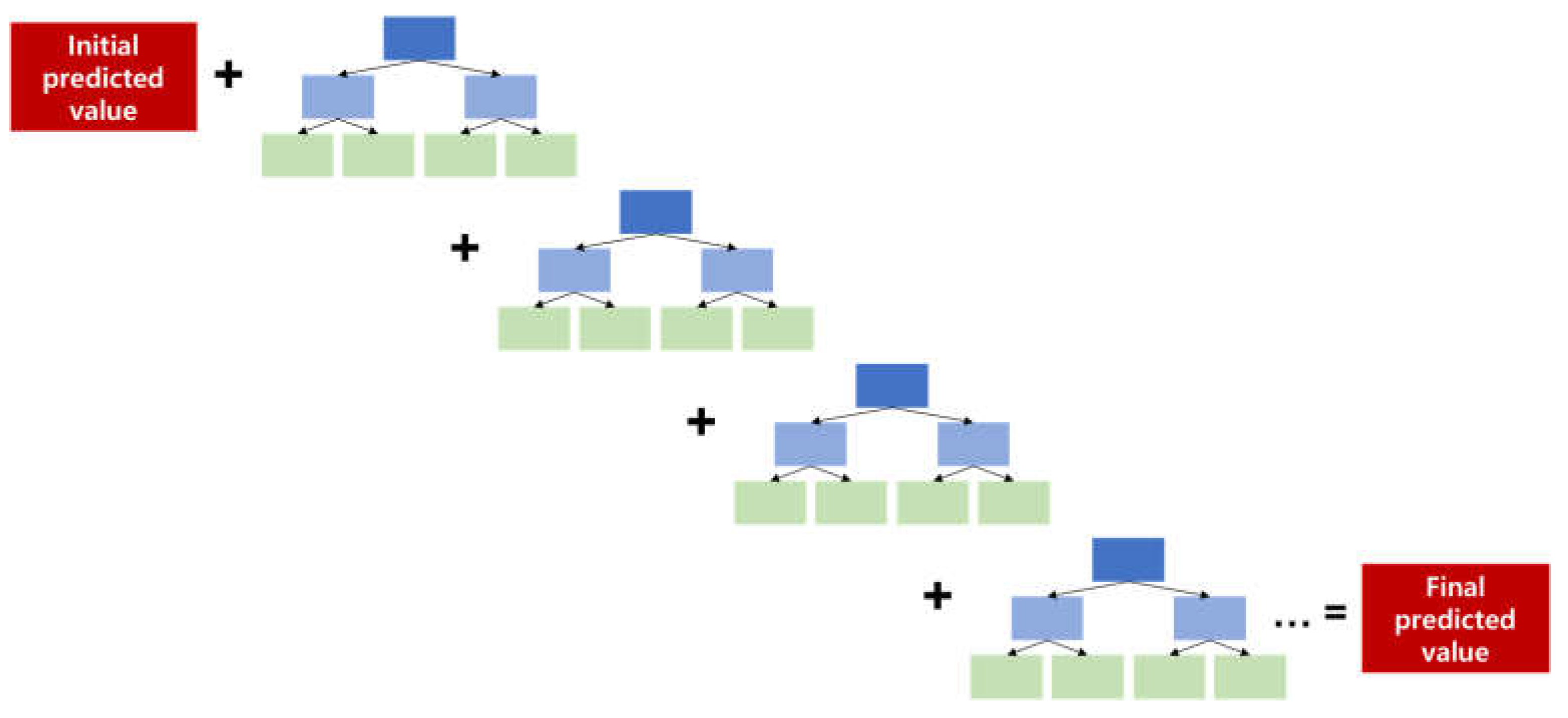
Figure 1 below is a simple schematic diagram of the gradient boosting algorithm. First, the initial predicted value is set as the average of the actual value. Second, after generating the first tree based on the error between the actual and the initial predicted value, the error with the actual value is calculated. Next, a second tree is generated based on the calculated error, and then the error with the actual value is calculated again. After repeating the above process as many as the total number of times settled in hyperparameter, the final prediction is derived by reflecting the learning rate on each tree.
Equation (1) below shows how to calculate final predicted value for each observation. As explained above, when the initial predicted value is determined as
, the error of each tree
is calculated
times, and the learning rate
is reflected to each tree to sum up the error and final predicted value
is drawn.
| where |
: |
initial predicted value |
| |
: |
final predicted value |
| |
: |
learning rate |
| |
: |
predicted error of each tree |
| |
: |
the number of trees |
3. Building Models and Evaluation
3.1. Exploratory Data Analysis and Preprocessing
To build an energy generation prediction model, data observed at 15 spots across the country were used. The data were recorded with the interval of an hour from 00:00 on 1 January 2020 to 23:00 on 31 December 2021. The given data set consists of two types. The ‘basic data set (hereinafter referred to as data set B)’ consists of 8 variables, prediction time, energy generation quantity (the target value), clear sky global horizontal irradiance (cGHI), solar zenith angle (Szen), solar azimuth angle (Sazi), extraterrestrial radiation (Extl), predicted ground temperature (Temp_nwp), and predicted global horizontal irradiance (GHI_nwp). The ‘advanced data set (hereinafter referred to as data set A)’ contains about 60 additional weather variables such as cloud cover, ground atmospheric pressure, altitude, visibility etc.
The Step 1 of preprocessing procedure below is given and Step 2 to Step 5 are the additional procedure we added to build more accurate models.
Preprocessing procedure:
Step 1: Combining all data set B observed from the 15 spots and delete the observations with missing values.
Step 2: Combining data set B and data set A. It means that about 60 weather variables that only existed in data set A were added to data set B.
Step 3: Dealing with ‘GHI_sat’ variable. As the ‘GHI_sat’ is an observed value in the past, the value is substituted with the one that was recorded 48 hours ago.
Step 4: Checking missing values once again and substitute them with the data of the same time one day before.
Step 5: For some variables, normalizing and standardizing the data to construct models.
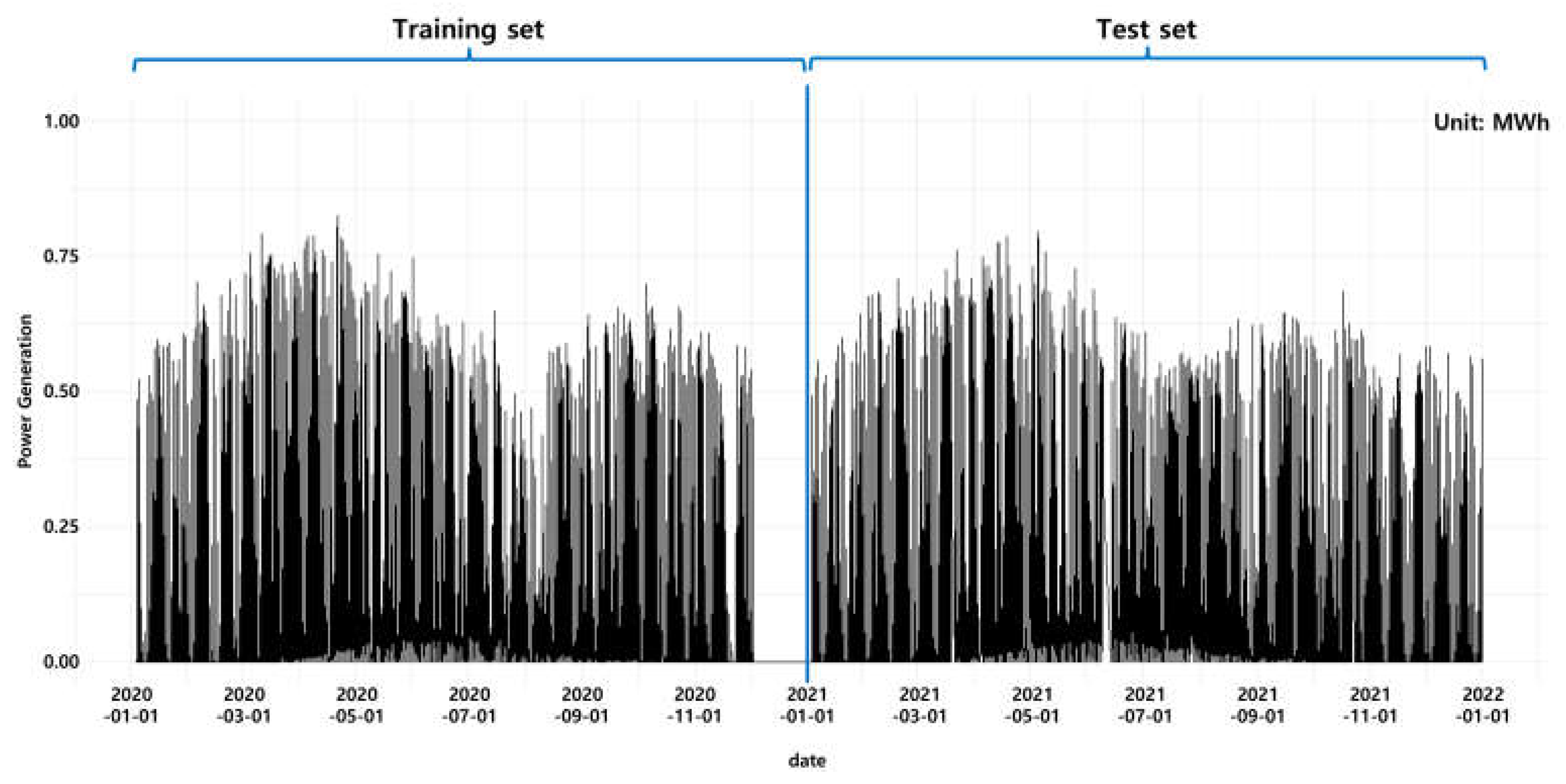
After going through the five preprocessing procedures for model construction, the data was separated into training data set and test data set. The training data set contains the data from 00:00 on 1 January 2020 to 23:00 on 31 December 2020, and the test data set contains the data from 00:00 on 1 January 2021 to 23:00 on 31 December 2021.
Figure 2 below shows the separation of target variable (energy generation quantity) from one of the 15 points.
3.2. Experiment
Table 1 below shows the various combinations of preprocessing procedure and the range of training data set applied to each model we made. In terms of preprocessing procedure, Model 2 and Model 3 went through more exquisite steps compared to Model 1. Also, the range of training data set used in model construction differs from the model. When building Model 1 and Model 2, the whole training data set was used while Model 3 was constructed with only upper 10% of energy generation capacity. By varying the properties of training data set in model building, we tried to compare which one showed the highest accuracy.
Unlike Model 1 and Model 2, data with an energy generation capacity of upper 10% were used among the training data set for Model 3. The reason why only upper 10% of energy generation capacity data was used for constructing Model 3 is the fact that the accuracy of energy generation prediction is calculated only with the data of upper 10% energy generation capacity [
16]. Therefore, we expected more accurate model construction would be possible if this criterion is applied to both model construction and accuracy calculation.
When constructing models, grid search was used for hyperparameter selection. The selected values are as follows. The same hyperparameter values was applied to all three models so that it would be able to guarantee an objectivity of evaluating the performance of the models.
The total number of threes: 500
The maximum depth of each tree: 10
The minimum number of samples for the terminal node of each tree: 20
Learning rate: 0.05
3.3. Evaluating Accuracy of Energy Generation Prediction Model
In this study, nMAE was used as a measure to evaluate the accuracy of the energy generation prediction model, which is officially used in the energy generation prediction system. MAE refers to the average of absolute errors between the actual value and the predicted value, and nMAE is an index that normalizes the MAE. In other words, since the difference between the actual and the predicted value is an evaluation index of accuracy in nMAE, the smaller the value, the more precisely the model is considered to have predicted the actual value.
Table 2 below shows the nMAE of three models (Model 1, Model 2, and Model 3) applied to the test data set from 00:00 on 1 January 2021 to 23:00 on 31 December 2021 for the 15 spots. In average, Model 2 has shown an nMAE of 8.41%, an improvement of 12.77% over nMAE of 9.64% in Model 1. In addition, the nMAE of Model 3 which was built with training data set of energy generation capacity of upper 10% was 8.08%, showing 16.14% better performance than Model 1. Moreover, it is remarkable that Model 3 showed an improvement compared to the Model 2, showing 3.87% higher accuracy. It is proved that model construction using training data set only with an energy generation capacity of upper 10% is more effective than using whole training data set.
With respect to each spot, all 15 spots showed an improvement in accuracy as the model develops from Model 1 to Model 3. Regardless of the types of models, spot 1 showed the highest accuracy with the nMAE of 7.69% for Model 1, 7.04% for Model 2, 6.70% for Model 3 respectively. In contrast, spot 3 showed the lowest accuracy with the nMAE of 11.48% for Model 1, 10.39% for Model 2, 9.90% for Model 3 respectively. As the model developed from Model 1 to Model 2, spot 14 showed the biggest improvement with the nMAE decrease of 15.81%. From Model 2 to Model 3, spot 12 improved the most with the nMAE decrease of 7.31%
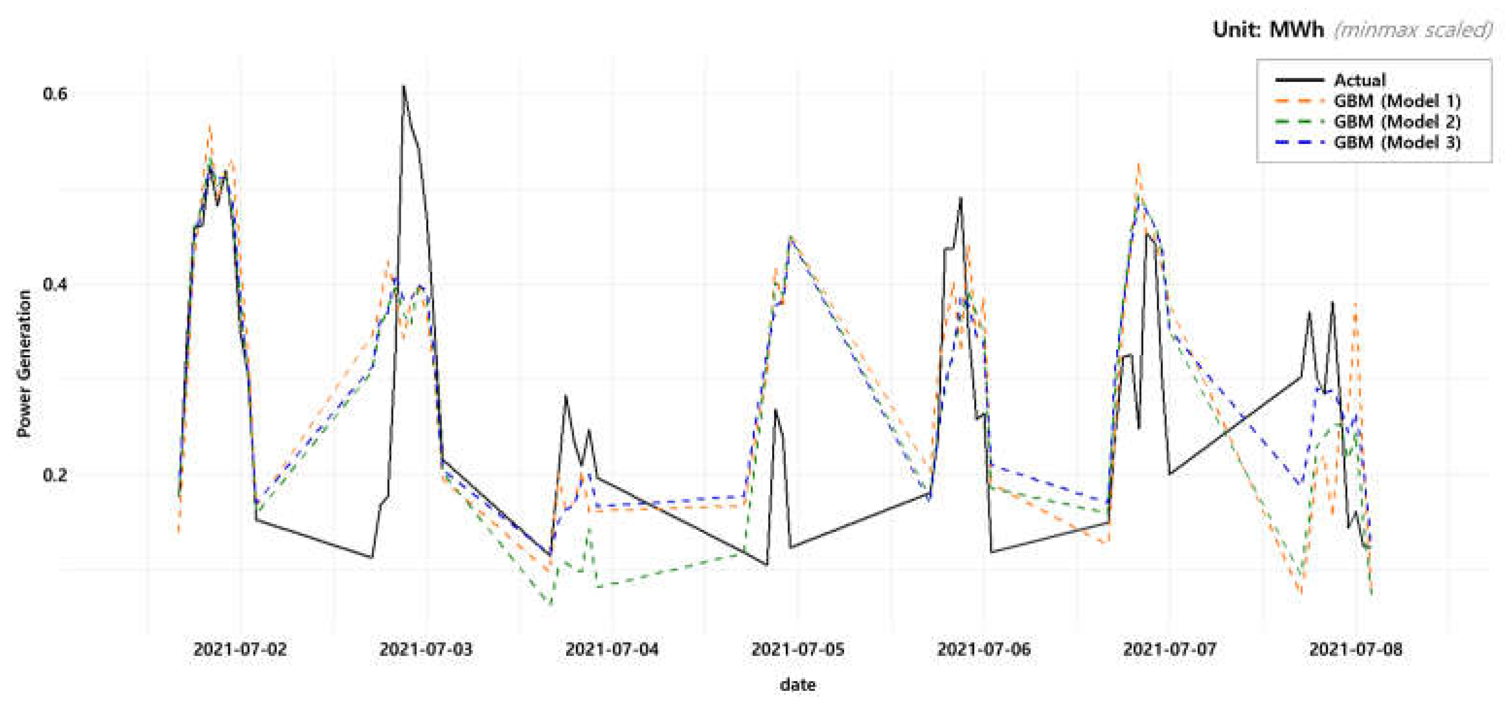
For the visual comparison of the three models,
Figure 3 below graphically shows the actual value of the energy generation (black solid line) and the values predicted with the three models (orange, green, and blue dotted line respectively) for some periods of time in test data set, which is from 00:00 on 1 July 2021 to 23:00 on 7 July 2021, for spot 0. Although the three models commonly showed a tendency to overestimate or underestimate in some certain periods of time, in general, the result showed that Model 3 derives the predicted value with the smallest error compared to the actual value.
4. Discussion
Traditionally, time series analysis has been widely used for the prediction of solar energy generation. Using the same data, one of time series analysis methods, autoregressive integrated moving average (hereinafter referred to as ARIMA) was conducted and the accuracy was compared with Model 1, Model 2, and Model 3.
4.1. ARIMA
The ARIMA model uses past observations, errors, and a difference procedure to explain current values. It includes both autoregressive (AR) model and the moving average (MA) model. A time series observation
follows the
process, where
is the parameter of AR model,
is a differential parameter, and
equals to the parameter of MA model respectively. When the mean value of
equals to
, the equation of ARIMA model is as follows. In this case,
and
are the polynomials for AR and MA model respectively,
indicates back shift operator.
| where |
|
| |
|
| |
|
| |
|
More precise explanation of each parameter is as follows.
p: The parameter for AR model. The observation value of time points affect the time point value.
d: The parameter for differencing. The observation value of time point is deducted from time point value to make the data stationary.
q: The parameter for MA model. The error of the continuous observation value affect the time point value.
After testing whether the data satisfies stationarity, parameter
are inferred by calculating the corrected Akaike’s information criterion (hereinafter referred to as AICc) of potential model. The residual analysis method, which tests the independence of the residuals by calculating the ACF and PACF of the residuals, is mainly used as a statistical diagnosis method to determine the appropriateness of the inferred model. Finally, we predict future time prediction values using the constructed model as a prediction model. In this study, we used AICc to test appropriateness when inferring the parameter
. Compared to Akaike’s information criterion (AIC), AICc is an index where a penalty is added with the number of parameters.
Table 3 below shows the 15 time series models for each spot with training data set. Like GBM, the training data set contains the data from 00:00 on 1 January 2020 to 23:00 on 31 December 2020, and the test data set contains the data from 00:00 on 1 January 2021 to 23:00 on 31 December 2021.
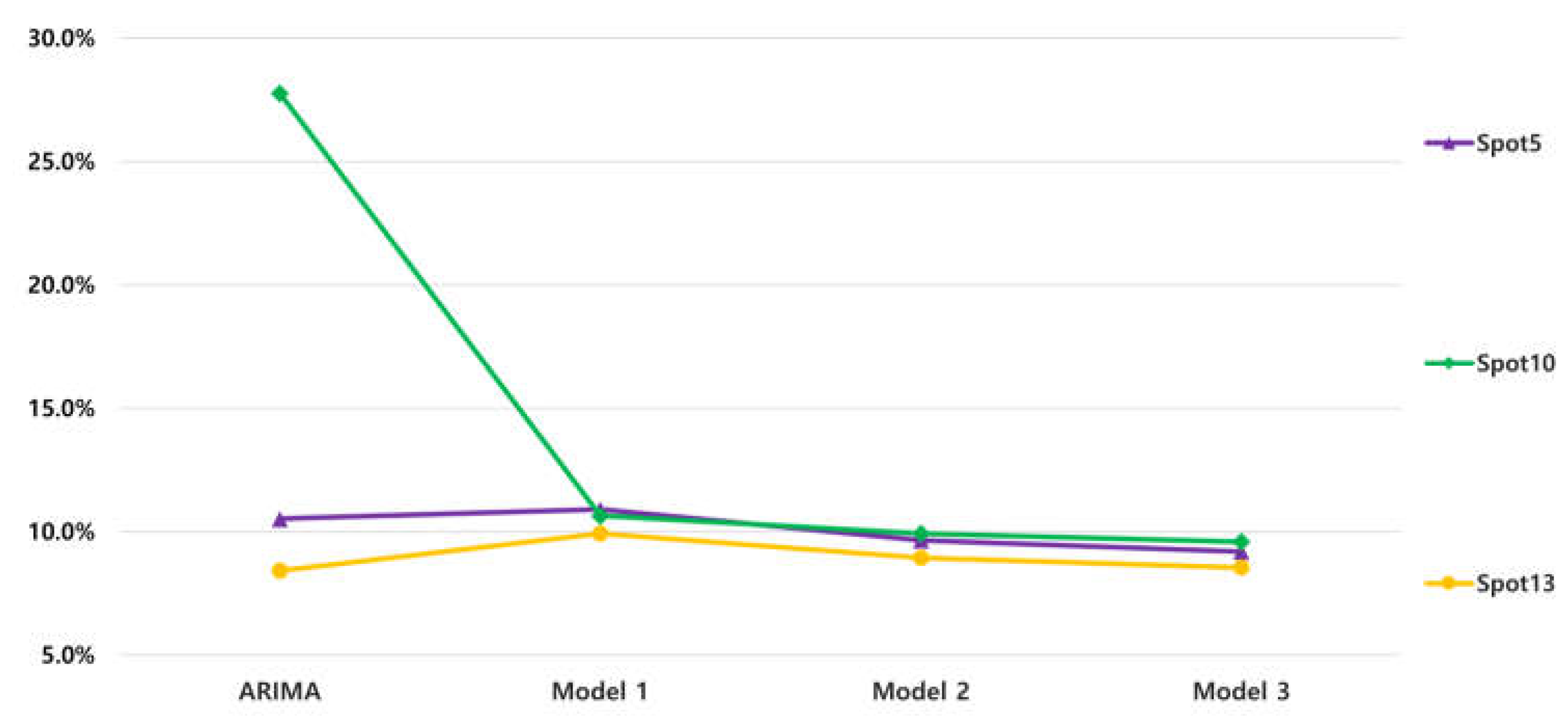
Table 4 below shows the nMAE of ARIMA of the model evaluation period, which is the period of test data set, containing the data from 00:00 on 1 January 2021 to 23:00 on 31 December 2021. Spot 13 showed the highest accuracy with the nMAE of 8.42%, while spot 10 showed the lowest accuracy with the nMAE of 27.76%.
5. Conclusion
In this study, using GBM, three regression models that predict solar energy generation were built and an experiment was conducted to compare prediction accuracy with nMAE. The difference between three models lies on the preprocessing method and the range of training data set. By differing the preprocessing procedure and the range of training data set, the intention was to compare which combination of data engineering method makes the most accurate result.
Experiment has shown that Model 2, with some additional preprocessing procedure compared to Model 1, has a better prediction performance. In addition, considering the fact that nMAE in the renewable energy generation prediction system is calculated only with the data with upper 10% of the energy generation capacity, a Model 3 was built in the same way but only data with upper 10% of the energy generation capacity were used as training data set. As a result, Model 3 even showed a higher performance compared to Model 2, as well as Model 1. The experiment showed that nMAE of Model 1, Model 2, and Model 3 was 9.64%, 8.41%, and 8.08% respectively.
Compared to Model 1, Model 2 went through additional preprocessing procedures so that it can predict solar energy generation more accurately. These additional preprocessing procedures include combining extra information, adjusting timeline of certain weather variable, normalizing and standardizing the data. This difference makes Model 2 to be more adequate for solar energy prediction, as the nMAE got better by 12.77%. Moreover, in contrast with Model 1 and Model 2, Model 3 was constructed with upper 10% of the energy generation capacity. By handling the range of training data set to match it with the range of accuracy calculation, it was able to derive the achievement with 16.14% of nMAE reduction compared to Model 1, 3.87% of nMAE reduction compared to Model 2 respectively.
For further analysis, a time series analysis has been conducted for the comparison with three GBM models.
Table 5 below shows the nMAE of ARIMA and three GBM models. Overall, compared to ARIMA, three models with GBM showed higher accuracy. Among the three models built with GBM, as the model develops from Model 1 to Model 3, the nMAE showed a progressive improvement with its decrease.
Figure 4 shows a graph of nMAE for each model of three remarkable spots. About spot 10, compared to the ARIMA, three models with GBM showed a dramatical reduction of nMAE. From ARIMA to Model 1, the nMAE decreased by 61.66%. With respect to spot 5 and spot 13, it is phenomenal that ARIMA showed higher accuracy than GBM models. Especially in spot 13, the nMAE of ARIMA recorded 8.42%, which is the smallest nMAE among the four models.
In the future, to build a model with a higher accuracy, we would like to build models with weather variables that have a great influence on energy generation prediction. In this study, we used all the variables from the given data. However, if some weather variables that have a large impact on energy generation prediction are selected using the concept of variable importance and then the model is built with only those variables, it will not only improve the model performance but also shorten the time required to build the model. Several studies have already proved that solar irradiance and atmospheric temperature has a great influence on solar energy generation [
17,
18].
In addition, rather than building prediction models for 15 spots respectively, clustering the spots into some number of groups regarding their geographical or climate feature would be a meaningful trial to expect more accurate models.
Author Contributions
Conceptualization, Yoo-Jung Kim, Na-Hyeong Kim and So-Yeon Park; Data curation, Jin-Young Kim, Chang-Ki Kim, Myeong-Chan Oh and Hyun-Goo Kim; Formal analysis, Yoo-Jung Kim, Na-Hyeong Kim, So-Yeon Park and Yung-Seop Lee; Funding acquisition, Jin-Young Kim, Chang-Ki Kim, Myeong-Chan Oh, Hyun-Goo Kim and Yung-Seop Lee; Investigation, Jin-Young Kim, Chang-Ki Kim, Myeong-Chan Oh, Hyun-Goo Kim and Yung-Seop Lee; Methodology, Yoo-Jung Kim, Na-Hyeong Kim and So-Yeon Park; Project administration, Jin-Young Kim, Chang-Ki Kim, Myeong-Chan Oh and Hyun-Goo Kim; Resources, Jin-Young Kim, Chang-Ki Kim, Myeong-Chan Oh and Hyun-Goo Kim; Software, Yoo-Jung Kim, Na-Hyeong Kim and So-Yeon Park; Supervision, So-Yeon Park and Yung-Seop Lee; Validation, Yung-Seop Lee; Visualization, Yoo-Jung Kim and Na-Hyeong Kim; Writing – original draft, Yoo-Jung Kim; Writing – review & editing, Jin-Young Kim, Chang-Ki Kim, Myeong-Chan Oh, Hyun-Goo Kim and Yung-Seop Lee. All authors will be informed about each step of manuscript processing including submission, revision, revision reminder, etc. via emails from our system or assigned Assistant Editor.
Funding
This was an award-winning work by participating in the “KIER Solar Prediction Academic Competition” which was jointly hosted by Korea Institute of Energy Research (KIET) and The Korean Solar Energy Society (KSES). This is supported by the National Research Foundation of Korea (NFR) grant funded by the Korea government (No. NRF-2021R1A2C1007095).
Data Availability Statement
Not applicable.
Conflicts of Interest
The authors declare no conflict of interest.
References
- Hwang, J.-Y. ; Korea Electric Power Corporation Home Page. Available online: https://home.kepco.co.kr/kepco/front/html/WZ/2022_01_02/sub13.html (accessed on 19 April 2023).
- Jung, A.-H.; Lee, D.-H.; Kim, J.-Y.; Kim, C.-K.; Kim, H.-G.; Lee, Y.-S. Regional Photovoltaic Power Forecasting Using Vector Autoregression Model in South Korea. Energies 2022, 15, 7853. [Google Scholar] [CrossRef]
- Zhang, P.; Takano, H.; Murata, J. Daily Solar Radiation Prediction Based on Wavelet Analysis. In Proceedings of the SICE Annual Conference (IEEE), Tokyo, Japan, 13-18 September 2011. [Google Scholar]
- Oudjana, S.H.; Hellal, A.; Mahamed, I.H. Short Term Photovoltaic Power Generation Forecasting Using Neural Network. In Proceedings of the 11th International Conference on Environment and Electrical Engineering (IEEE), Venice, Italy, 18-25 May 2012. [Google Scholar]
- Kim, Y.-S.; Lee, S.-H.; Kim, H.-W. Prediction Method of Photovoltaic Power Generation Based on LSTM Using Weather Information. The Journal of Korean Institute of Communications and Information Sciences 2019, 44, 2231–2238. [Google Scholar] [CrossRef]
- Lee, S.-M.; Lee, W.-J. Development of a System for Predicting Photovoltaic Power Generation and Detecting Defects Using Machine Learning. KIPS Transactions on Computer and Communication Systems 2016, 5, 353–360. [Google Scholar] [CrossRef]
- Yona, A.; Senjyu, T.; Funabashi, T. Application of Recurrent Neural Network to Short Term-ahead Generating Power Forecasting for Photovoltaic System. In Proceedings of the 2007 IEEE Power Engineering Society General Meeting (IEEE), Tampa, Florida, USA, 24-28 June 2007. [Google Scholar]
- Yona, A.; Senjyu, T.; Funabshi, T.; Sekine, H. Application of Neural Network to 24-hours-ahead Generating Power Forecasting for PV System. In Proceedings of the 2008 IEEE Power and Energy Society General Meeting - Conversion and Delivery of Electrical Energy in the 21st Century, Pittsburgh, Pennsylvania, USA, 20-24 July 2008. [Google Scholar]
- Capizzi, G.; Napoli, C.; Bonanno, F. Innovative Second-generation Wavelets Construction with Recurrent Neural Networks for Solar Radiation Forecasting. IEEE Transactions on Neural Networks and Learning Systems 2012, 23, 1805–1815. [Google Scholar] [CrossRef] [PubMed]
- Cao, S.; Weng, W.; Chen, J.; Liu, W.; Yu, G.; Cao, J. Forecast of Solar Irradiance Using Chaos Optimization Neural Networks. In Proceedings of the 2009 Asia-Pacific Power and Energy Engineering Conference (IEEE), Wuhan, China, 28-30 March 2009. [Google Scholar]
- Mellit, A.; Pavan, A.M. A 24-hour Forecast of Solar Irradiance Using Artificial Neural Network: Application for Performance Prediction of a Grid-connected PV Plant at Trieste, Italy. Solar Energy 2010, 84, 807–821. [Google Scholar] [CrossRef]
- Wang, F.; Mi, Z.; Su, S.; Zhao, H. Short-term Solar Irradiance Forecasting Model Based on Artificial Neural Network Using Statistical Feature Parameters. Energies 2012, 5, 1355–1370. [Google Scholar] [CrossRef]
- Hocaoğlu, F.O.; Gerek, Ö.N.; Kurban, M. Hourly Solar Radiation Forecasting Using Optimal Coefficient 2-D Linear Filters and Feed-forward Neural Networks. Solar Energy 2008, 82, 714–726. [Google Scholar] [CrossRef]
- Yun, Z.; Quan, Z.; Caixin, S.; Shaolan, L.; Yuming, L.; Yang, S. RBF Neural Network and ANFIS-based Short-term Load Forecasting Approach in Real-time Price Environment. IEEE Transactions on Neural Networks and Learning Systems 2008, 23, 853–858. [Google Scholar] [CrossRef]
- Ke, G.; Meng, Q.; Finley, T.; Wang, T.; Chen, W.; Ma, W.; Ye, Q. Light GBM: A Highly Efficient Gradient Boosting Decision Tree. In Proceedings of the Advanced in Neural Information Proceeding System 30 (NIPS), Red Hook, New York, USA, 4-9 December 2017. [Google Scholar]
- Korea Power Exchange Home Page. Available online: https://der.kmos.kr/intro/fr_intro_view10.do (accessed on 19 April 2023).
- Huang, Y.; Lu, J.; Liu, C.; Xu, X.; Wang, W.; Zhou, X. Comparative Study of Power Forecasting Methods for PV Stations. In Proceedings of the International Conference on Power System Technology (IEEE), Zhejiang, Hangzhou, China, 24-28 October 2010. [Google Scholar]
- Chen, C.; Duan, S.; Cai, T.; Liu, B. Online 24-h Solar Power Forecasting Based on Weather Type Classification Using Artificial Neural Network. Solar Energy 2011, 85, 2856–2870. [Google Scholar] [CrossRef]
|
Disclaimer/Publisher’s Note: The statements, opinions and data contained in all publications are solely those of the individual author(s) and contributor(s) and not of MDPI and/or the editor(s). MDPI and/or the editor(s) disclaim responsibility for any injury to people or property resulting from any ideas, methods, instructions or products referred to in the content. |
© 2023 by the authors. Licensee MDPI, Basel, Switzerland. This article is an open access article distributed under the terms and conditions of the Creative Commons Attribution (CC BY) license (http://creativecommons.org/licenses/by/4.0/).


