Geological Mapping of Grib Kimberlite Pipe Using 3D Magnetization Vector Inversion From Airborne Data

Preprint

Case Report

Geological Mapping of Grib Kimberlite Pipe Using 3D Magnetization Vector Inversion From Airborne Data

Altmetrics

Downloads

122

Views

Comments

Vladislav Kaminski^*,Valeriya Nabieva,Alexander Frolov,Inna Shalovenkova,

Alexander Davydenko

Vladislav Kaminski^*,Valeriya Nabieva,Alexander Frolov,Inna Shalovenkova,

Alexander Davydenko

This version is not peer-reviewed

Submitted:

09 June 2023

Posted:

09 June 2023

You are already at the latest version

Alerts

Abstract

This study is describing airborne geophysical survey, carried out in Northeastern Russia (Archangelsk region) in order to aimed at geological mapping of Grib kimberlite pipe, which is known to have strong presence of remanent magnetization. Airborne data were inverted using two techniques, the magnetization vector inversion (MVI) and a QDIK inversion, a proprietary algorithm developed at the Irkutsk State University (ISTU), which allows extracting four parameters from airborne magnetic data (magnetic susceptibility, inclination, declination and Koeniksberger ratio). The inversion results were further analyzed and verified against the known geology of the Grib kimberlite. The study allowed to better map geology of Grib kimberlite using only uninvasive (remote sensing) technology

Keywords:

Subject: Environmental and Earth Sciences - Geophysics and Geology

1. Introduction

Grib kimberlite pipe is located in the Archangelsk diamondiferous province (north of European Russia). It was discovered in 1996 and is now one of major diamond producing mines in Russia [1]. It has estimated reserves of 98.5 million carats of diamonds and an annual production capacity of 3.62 million carats. Its surface area is measured more than 16 hectares and is traced by drilling operations to the depth of 1024 m. Since its discovery, the pipe has been a subject to multiple remote sensing and geophysical surveys, photogrammetry as well as extensive drilling operations, which allowed constructing an accurate geological model. All remote sensing and geophysical data sets collected since 1996 were in some way subject to cultural and/or industrial disturbance [2]. The study of the pipe itself is further complicated by the overlaying 60-80 m thick Cretaceous sediments, which make its mapping impossible using satellite remote sensing and photogrammetry techniques and challenging even with usage of airborne magnetometry.

Generally, kimberlitic pipes, which are the main sources of diamonds consist of three facies: root (deeper) facies, diatreme facies, and crater (upper) facies [3]. In many cases, the pipes are eroded to some extent, and usually the diatreme facies, composed by hypabyssal kimberlite with typical magmatic structure and composition, emerges at the surface level. However, in some areas, kimberlite with lesser degree of erosion may expose bowl-shaped crater zone at the surface, formed by a variety of eruptive and resedimentation processes. The kimberlitic material of the crater facies is often diluted with sedimentary material, making it difficult to identify by direct observations, remote sensing and geophysical methods.

1.1. Geology

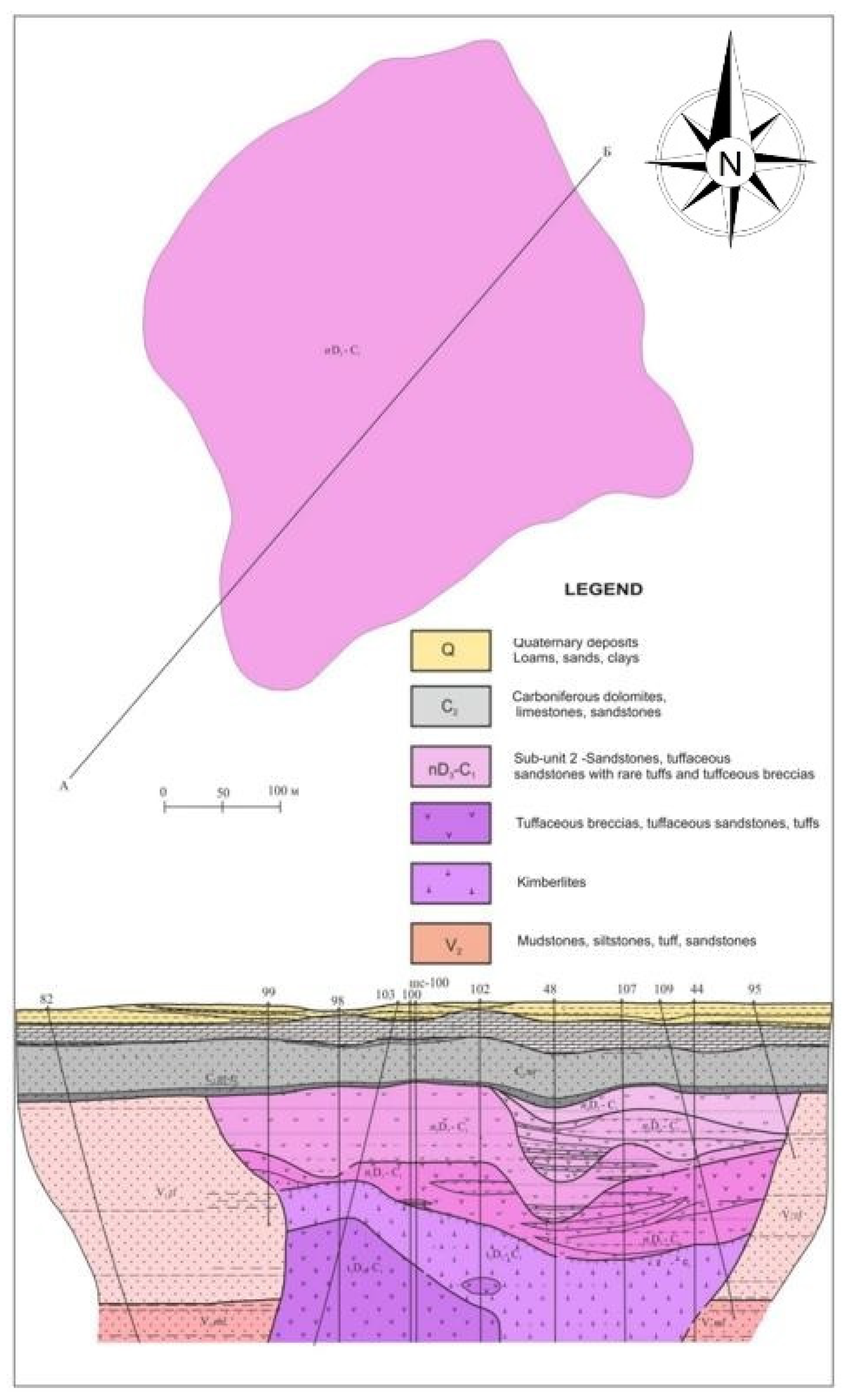
Grib pipe is located in central part of Zimniy bereg (Winter shore) diamondiferous province within Chernoozersky kimberlite field. It was formed during D₂-C₁ magmatism, cutting through Rifean and Vendian sedimentary strata and is overlain by terrigenous-carbonate formation of middle Cretaceous age, which, in turn, is overlain by loose quaternary sediments (Figure 1).

Rifean sysem is represented by interbedded silts and clays with thin lenses of variegated sandstones. Its estimated thickness is 50 – 70 m.

The upper Vendian system is composed of four suites: Ust-Pinezhskaya (V₂up); Erginskaya (V₂er) Melskaya (V₂ml) and Zolotnickaya (V₂zl). V₂up is characterized by predominance of silts over sandstones with presence of three tuffaceous horizons. Estimated thickness of V₂up pack is 560 m. V₂er has thickness of 64 to 87 m while V₂ml has thickness of 165 to 180 m. Both are composed of interbedded silts and sandstones. Perhaps the thickest pack of sediments is V₂zl reaches up to 400 m in thickness and is composed of red-coloured fine-grained sandstones with interbeds of silts.

Middle Cretaceous and Quaternary rocks are directly overlaying the kimberlite pipe with Cretaceous system reaching 52 to 82 m and comprised of uniform quartz sandstones slightly mixed with gravel material at the base of the pack.

Quaternary system is composed of sands, sandy loams and clays and reaches from 0.4 to about 20 m in thickness. There are unstratified dolomites and dolomitic limestones present directly below quaternary pack varying in thickness from 10 to 30 m.

The kimberlitic rocks of Grib pipe can be conditionally stratified into crater and hypabyssal facies. Crater facies is the shallowest part of the kimberlite with depths interval from 52 to 209 m (averaging 100 m in thickness). It is composed of various rocks including sandstones mixed with igneous material, tuffaceous sandstones, tuffs and sedimentary breccias.

Hypabissal facies can be followed to depths exceeding 1000 m below surface and is composed of two types of material. The upper part of hypabyssal facies is composed of kimberlitic tuff breccias, the other type is pure kimberlite. Thin carboniferous veins are widely present. The contact of kimberlite with host rocks are sharp with abrupt and clear transitions [1].

1.2. Magnetic properties

This section is mainly based on research of paleomagnetic properties of the rocks composing the Grib pipe, as well as the host rocks present within the survey area carried out by VNIGRI Russian Research Institute of Oil and Mineral exploration [4].

The magnetic properties of rock types from area under study have a very wide range. (Table A1) contains scalar characteristics of J_n (magnitude of natural remanent magnetization measured in A/m); K_m (magnetic susceptibility in SI units); Q (Koeniksberger ratio); Inclination (I_o); Declination (D_o); statistical parameter describing likelihood that the values lie outside of 95% confidence range (α95), sample masses and direction of natural remanent magnetization of kimberlites and kimberlitic tuff breccias.

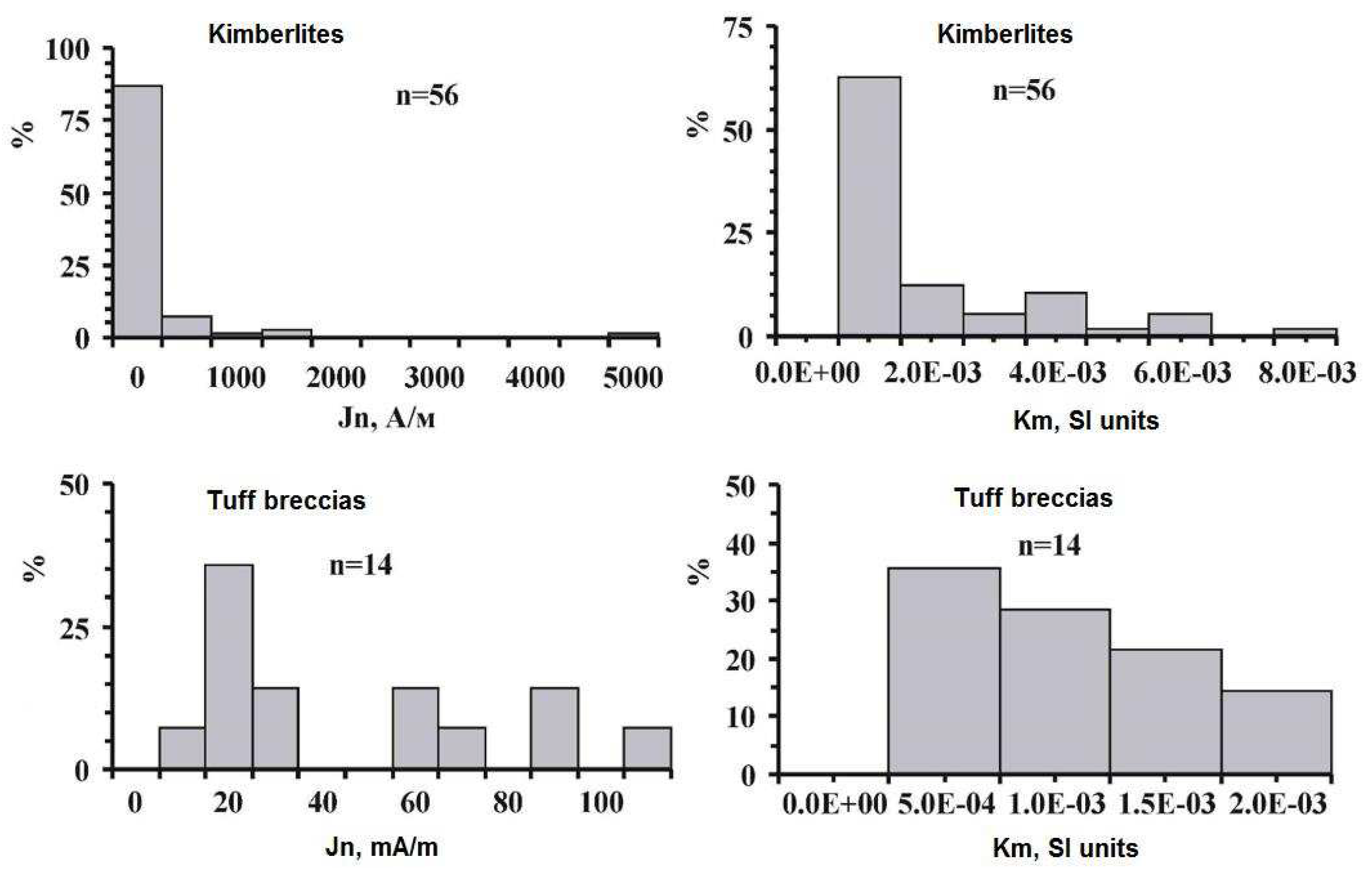
The histograms of J_n and K_m distribution are shown in Figure 2. Table 1 contains mean values and ranges of natural remanent magnetization and magnetic susceptibilities of kimberlite rock types from Grib pipe, Table 2 contains magnetic properties of host rocks from area under study.

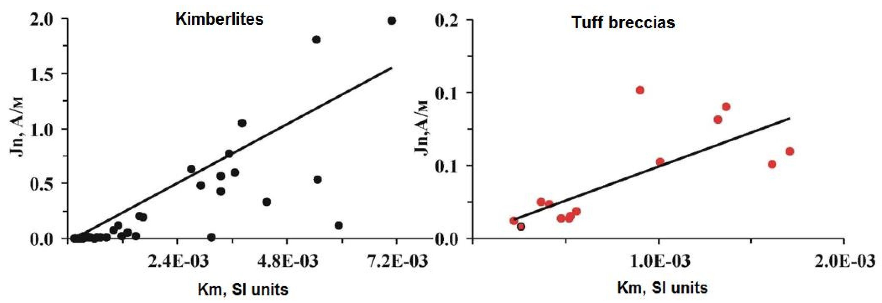
The relationships between scalar values of Jn with Km are shown in Figure 3. They form elongated groups with visible linear trend, which reflects concentration of magnetic minerals in the rock types. The latter may be attributed to potential preservation of primary paleomagnetic information. Some data from kimberlites and tuff breccias overlap.

The solid lines in Figure 3 represent averaged values forming linear trends.

Evaluation of induced magnetization (Ji) can be done without accounting for demagnetization coefficient due to body shape, as the values of magnetic susceptibility are low (Km <<0.1 SI units). Induced magnetization can be derived for each rock type using the mean values of Km from Table A1 and parameters of current magnetic field (HT) in the area of study (D = 17.9°; I = 77.3°; HT = 43.6 А/м at 65.5°N/41.4°E), Ji = Km*HT. The values of Ji are also provided in Table A1 on last lines of every rock type section and comprises 22% of the corresponding Jn values for kimberlites and 87% for kimberlitic tuff breccias and 24% for all other rock types.

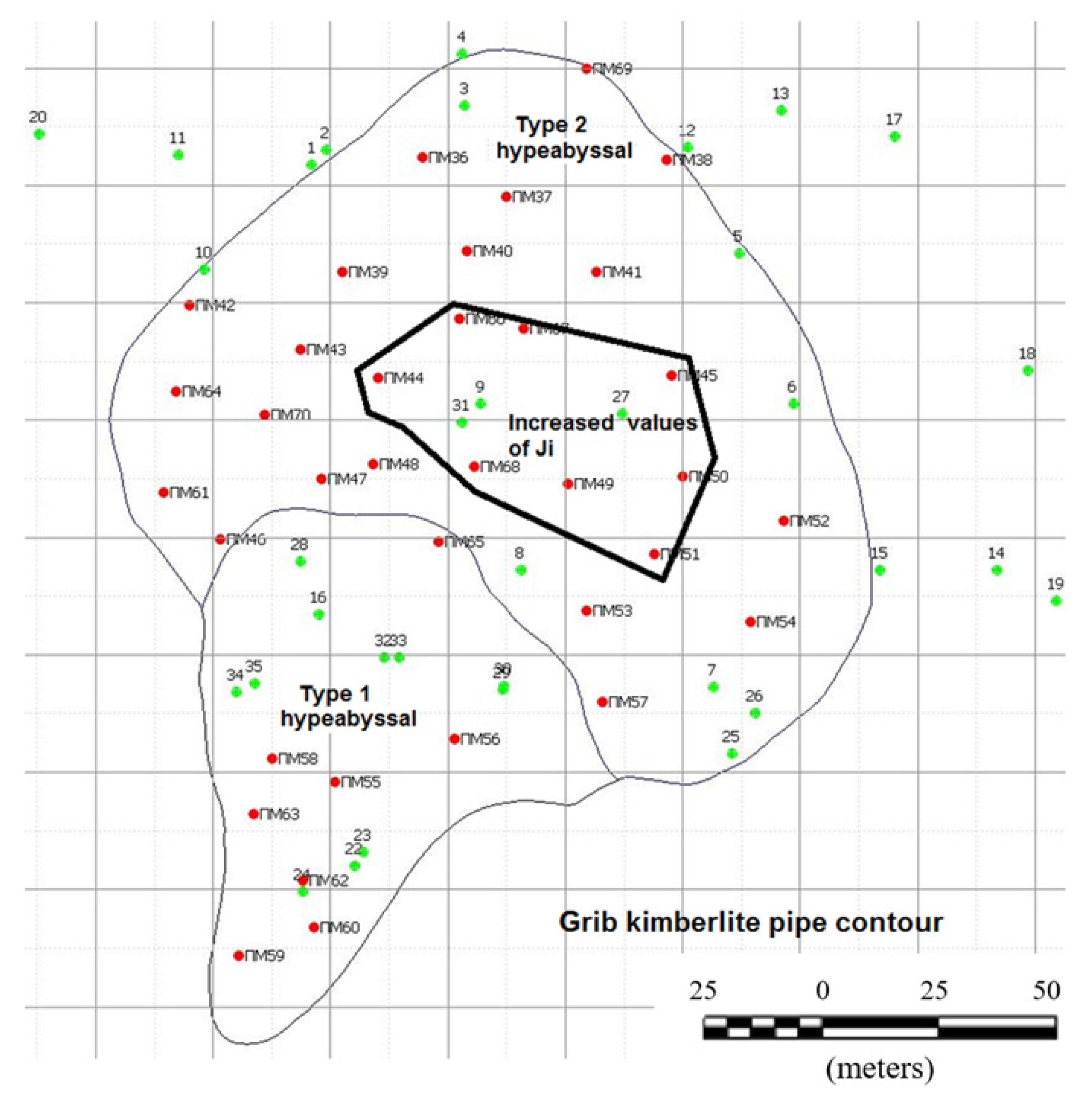
Considering wide spread of sample collection locations, Ji does not have significant effect on the area in general, however there is a narrow localization of significantly increased Ji values, following trend of samples 44, 45, 49, 50, 51. 66, 67 and 68 (Figure 4), which generally corresponds to central occurrence of type 2 (consolidated kimberlite) hypabyssal facies of Grib pipe.

Summarizing the materials presented in this section (more comprehensively studied in [4]) the following generalized statements can be made:

Sampled rocks have the following average values: J_n = 2.32Е-01 А/m, K_m = 1.29E-03 SI units. а. J_i=43.6∙1.29E-03=5.61E-02 А/m.
The highest average values recorded in kimberlites are as following: J_n = 2.80E-01 А/m, K_m= 1.41E-03 SI units, J_i = 43.6∙1.41E-03 = 6.13E-02 А/m.
Consolidated kimberlites form anomalous group of samples with high anisotropy of magnetic susceptibility (P = 1.58). These samples are characterized by high values of J_n, reaching 5 A/m. On the map of Grib pipe these samples fall within a compact area elongated in NW-SE direction.
The distribution of J_n/K_m is best described by linear relationships, which, in turn, reflects concentration of magnetic minerals in sampled rock types.
The predominant magnetic minerals responsible for J_n are iron hydroxides (magnetite, titanomagnetite and hematite).
The directions of full natural remanent magnetization have a wide range. Both direct and reversed polarity is observed.
The average direction of induced magnetization of sampled rock types has been evaluated using anisotropy of magnetic susceptibility (D=27°, I=77°), which is consistent with direction of current magnetic field in the area under study, J_i = 43.6∙1.29E-03 = 5.61E-02 А/m

2. Materials and Methods

We made a comprehensive study of an airborne data set, which was collected in 1985, some 11 years prior to kimberlite pipe discovery. The airborne magnetic data set was aquired using a fixed-wing Antonov-2 aircraft with average terrain clearance of 120 m. There was no obvious response from the pipe in the 1995 airborne data, therefore the data were first subject to trend removal, then subject to two types of 3D geophysical inversions:

Magnetization vector inversion [5]
QDIK inversion for susceptibility and remanent magnetization [6]

Both resulting data sets were compared to known geology as well as to each other in order to establish correlation with kimberlite facies uncovered by drilling, as well as to suggest an improved routine for advanced interpretation of airborne magnetic data for kimberlite exploration in cases when remanent magnetization is present.

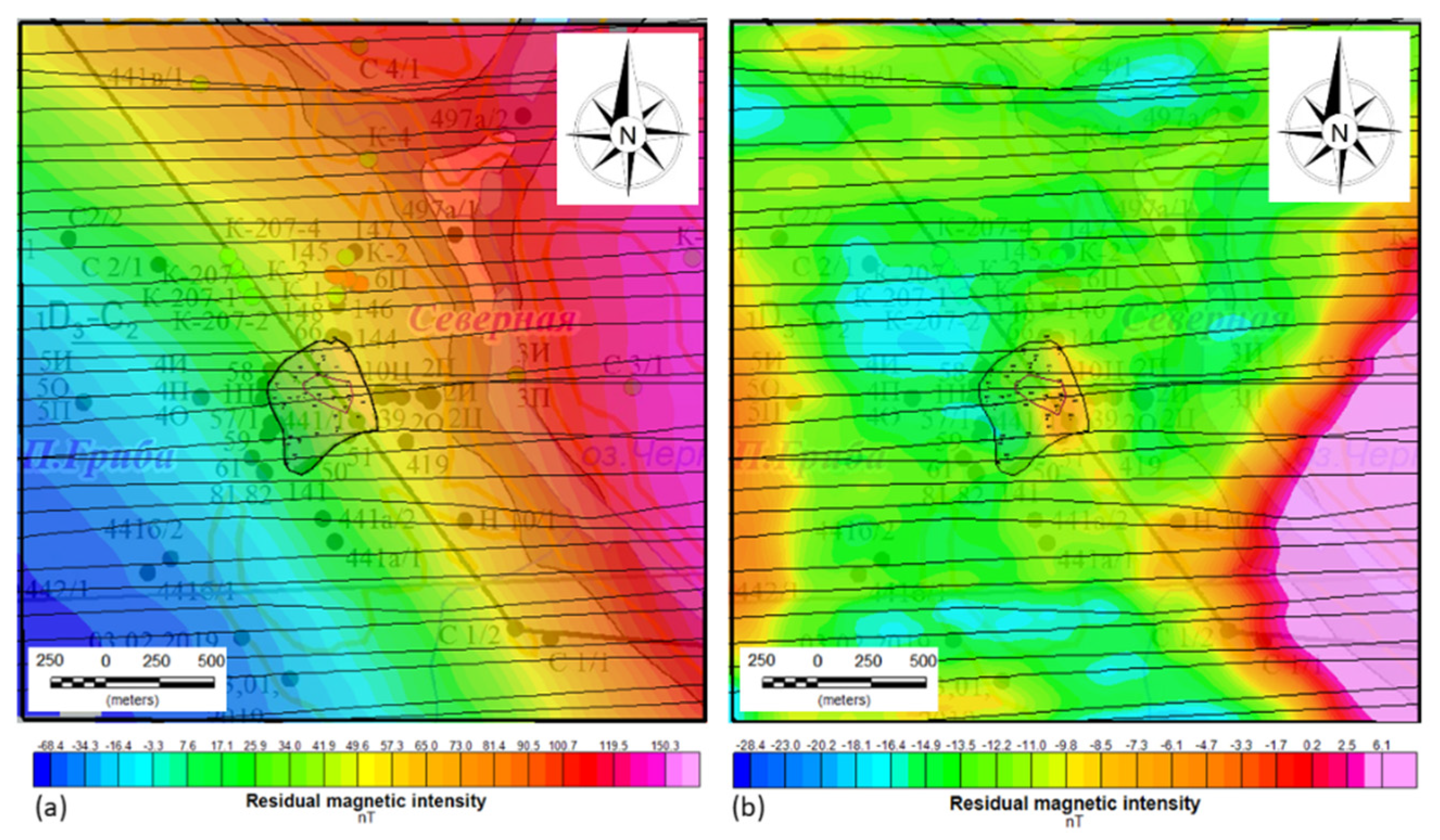
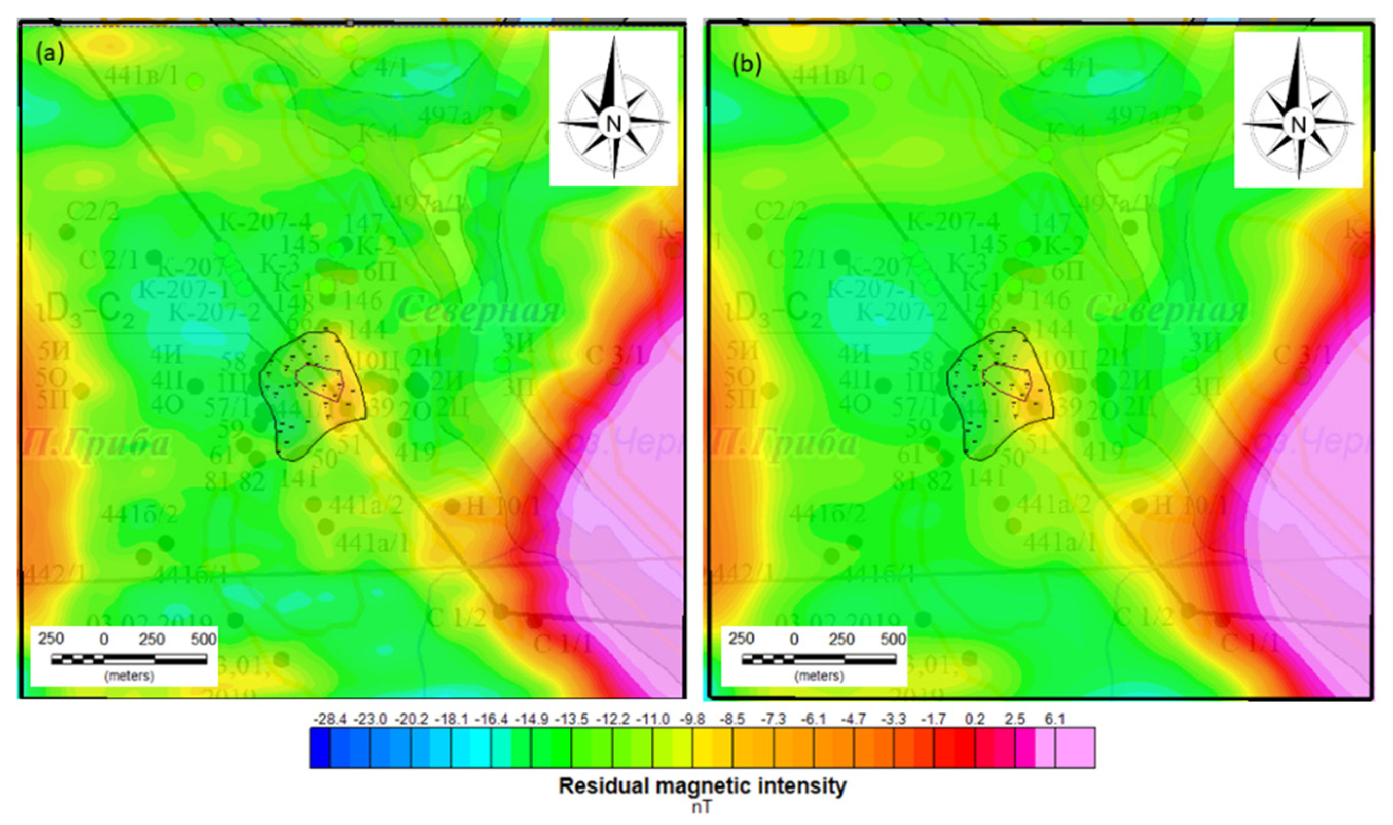
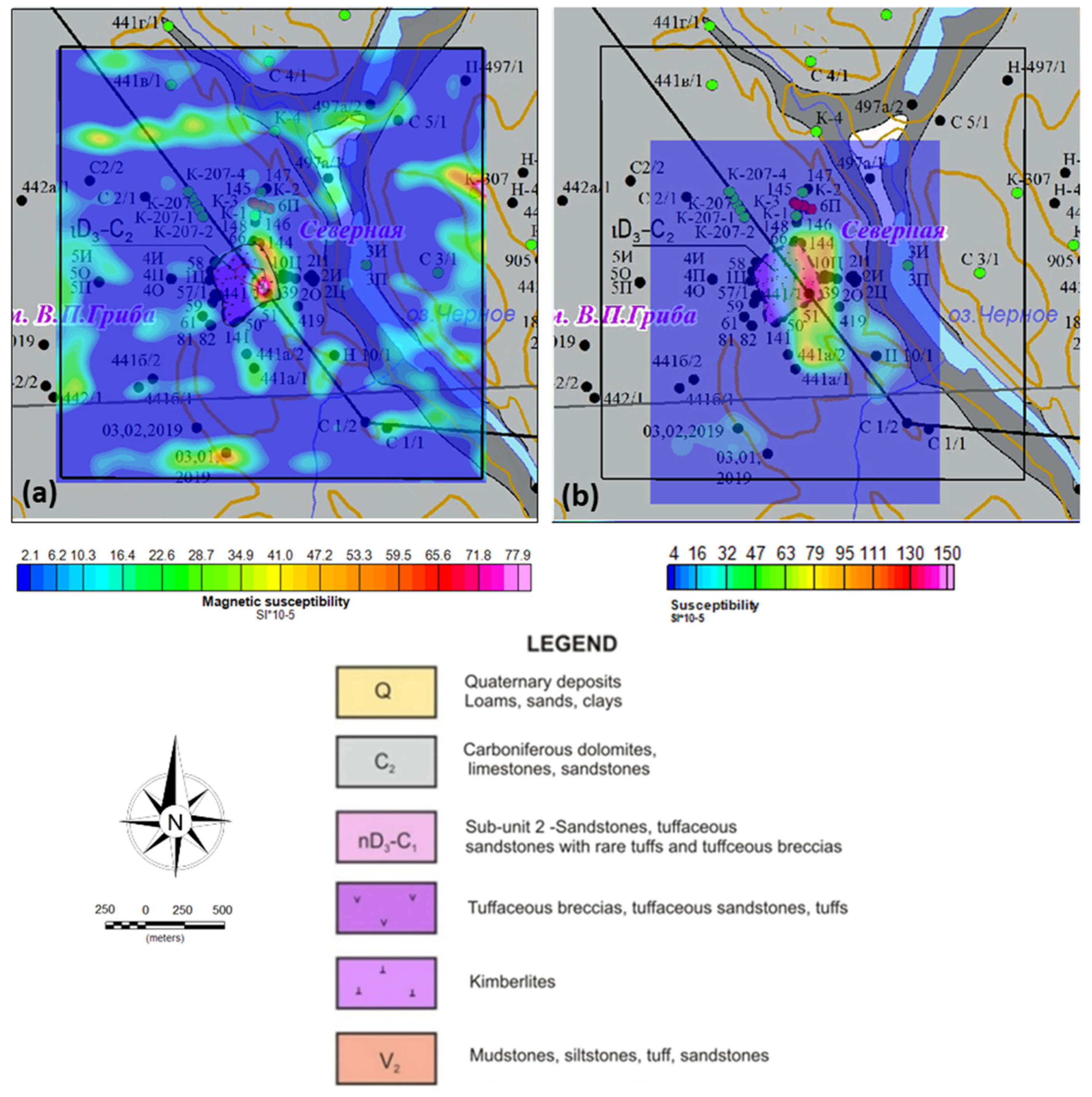
The total magnetic intensity data collected over Grib kimberlite pipe in 1985 are shown over bedrock geology in Figure 5а. The flight lines are trending EW and are rendered in black colour. As it can be seen from the figure, there is no obvious reflection of the pipe in the RMF data, therefore the data were subject to trend removal Figure 5b ,which resulted in some improvement in mapping the kimberlite, however with only fractional reflection of the target.

Methods of 3D magnetic data inversions described in this section include full magnetization vector inversions: MVI [5] and QDIK [6], which both allow to recover magnitude and direction of full magnetization vector J_t = J_i + J_n.

3. Results

3.1. MVI inversion

The abbreviation stands for Magnetization Vector Inversion [5]. This is a voxel (3D) inversion carried out on a regular rectangular mesh, which allows to recover both remanent and inductive magnetization by means of solving inverse problem for strength and direction of full natural magnetization from magnetic intensity data and without prior knowledge of the direction or strength of remanent magnetization. In majority of magnetic inversion algorithms it is assumed that the magnetic field is entirely a result of magnetic induction. In many field data sets however there are strong and obvious effects of remanent magnetization, including cases, when total magnetic intensity yields negative values.

Magnetic Induction B(r_j) is a vector field, which can be described in a form of equation (1) in magnetostatics [7]

B (r_{j}) = \nabla \int_{V} M (r) \cdot \nabla \frac{1}{|r - r_{j}|} d r^{3}

(1)

where r_j is the observation point; V is the volume containing magnetization vector M(r). In case of MVI inversion we invert B(r_j) for M(r) using Tikhonov minimum gradient regularizer (2):

M i n ϕ (m) = ϕ_{D} (m) + λ ϕ_{M} (m) ϕ_{D} (m) = \sum_{j}^{M} {|\frac{G_{j} m - B_{j}}{e_{j}}|}^{2} ϕ_{M} (m) = \sum_{Y}^{3} {|w_{Y} \partial_{Y} m|}^{2} + {|w_{0} m|}^{2} λ ∶ ϕ_{D} (m) = X_{T}^{2}

(2)

where 𝜙(m) is the total objective function, composed of data objective 𝜙D(m) and model objective function 𝜙M(m). The two parts of the total objective function are scaled using the trade-off parameter λ, which is chosen based on convergence of the routine in chi-squared sense χ². The data objective function includes the forward modelling operator G_jm, which is at each iteration step is compared with observed data B in order to fit within the assigned error e_j. The model objective function contains gradient of the model Δ_γm and the altitude of the model with weighting terms w_γ and w₀. In this routine additional constraints such as upper and lower bounds can be placed on m, which can be derived from a-priori information.

The TMI data collected over Grib pipe was subject to MVI inversion. The data set was optimized to accommodate one sample per mesh cell. A regular mesh measuring 208 x 210 x 153 cells in its core area was used for the MVI inversion with smallest cell measuring 15 x 15 x 10 m in X Y and Z directions accordingly. Padding of 665 m (6 cells starting from 32m m with expansion coefficient of 1.5) was allowed in every direction. Convergence to target misfit was achieved in 16 iterations).

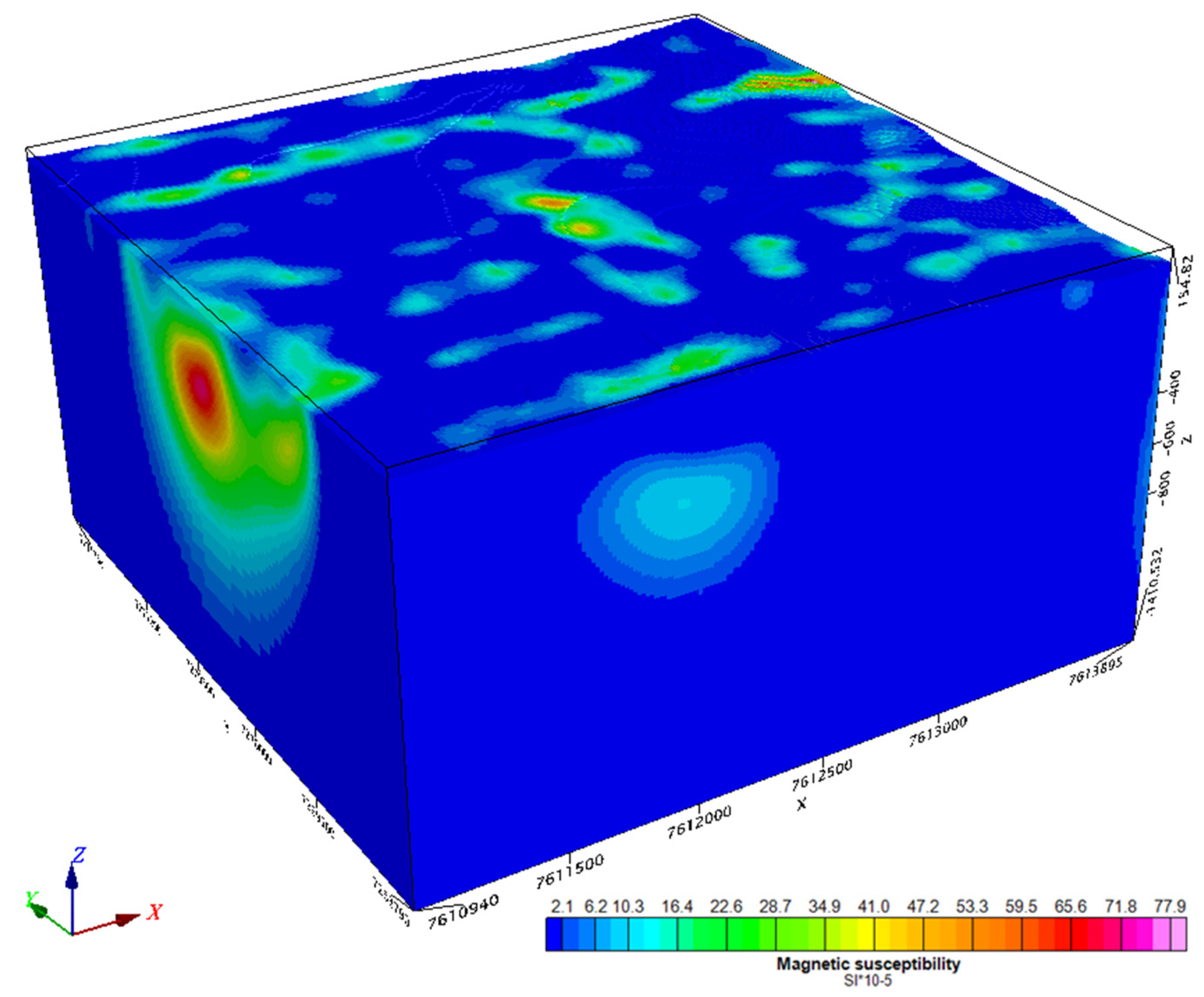
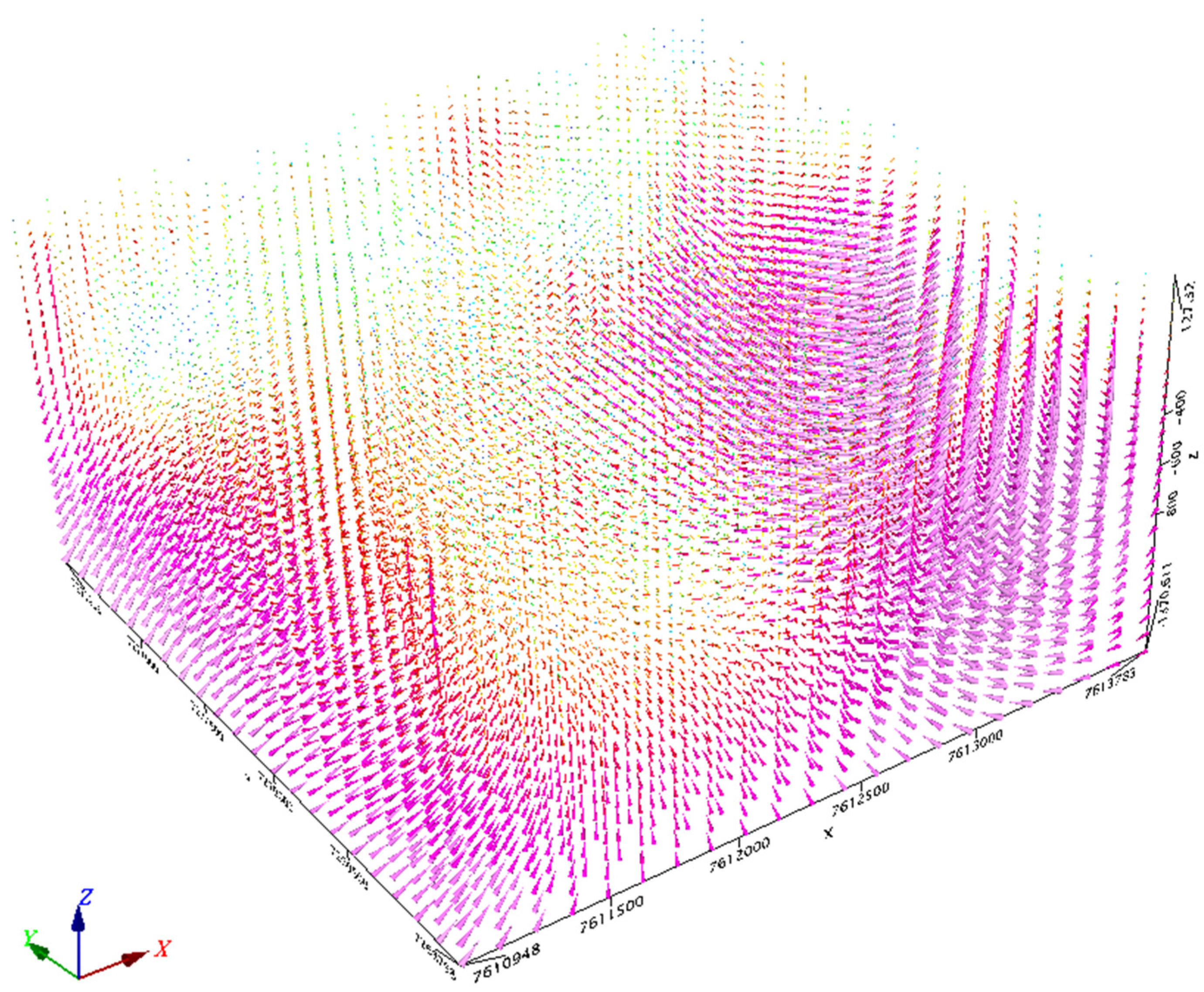
As a result, several voxel models were calculated including amplitude of magnetization vector. Corrected magnetic susceptibility values were calculated from magnetization amplitudes by using a multiplication factor of 43.6 (derived from the petrophysical studies). The susceptibility voxel model derived from MVI inversion is shown in Figure 6. Magnetization vector voxel model is shown in Figure 7. The data fit of MVI inversion is shown in Figure 8.

3.2. QDIK inversion

This is an example of so-called “cascade” inversion used on potential field data. The methodology described in this section is applied to magnetic data and describes recovery of both inductive and remanent components of magnetization vector from magnetic survey data by means of inversion using adaptive meshes [5,8,9]. This is a multiparametric inversion capable of recovering magnetic susceptibilities alongside (K) with Koeniksberger ratio (Q) and remanent Inclination (I) and Declination (D).

The possibility of global minimization of the residual field at a consecutive allocation of local objects, which provides a monotonous reduction of dispersion of the residual field is shown. For the inversion of the field in the local area, the algorithm of robust regression by the method of elastic network with the attraction of prior information on the physical properties of geological objects is used. Results of the inversion of the magnetic field allow defining magnetic susceptibility, and vector of residual magnetization of local objects, and density for the gravitational field.

The described algorithm uses different types of regularization of inverse problem, which allows accurate recovery of total magnetization vector unique for each mesh element. Regularization algorithms vary in boundary conditions and weighting functions incorporated in model objective function [9].

In order to separate inductive component of magnetization vector from remanent it is necessary to know the distribution of magnetic susceptibility over the area of modelling, therefore it is important to use a-priori information, which may be defined in form of other inversion results, range of predicted magnetic properties and possible shapes of the magnetized targets.

The following section describes the algorithm of the QDIK-inversion in greater details

Input data

Magnetic field data, corner coordinates, geometric and physical parameters of inversion models:

-

Anomalous magnetic $∆ T$ );

-

Digital elevation model and sensor height;

-

Normal magnetic field parameters ( $T_{0}$ – magnitude of normal magnetic field vector; $D_{0}$ – declination; $I_{0}$ – inclination);

-

A-priori petrophysical information as ranges of possible physical property values:

◦

Magnetic susceptibility ( $χ_{m i n}$ , $χ_{m a x}$ );

◦

Remanent magnetization vector parameters and their discretization: ( $∆ *$ ):

▪

Koeniksberger ratio ( $Q_{m i n}$ , $Q_{m a x}$ , $∆ Q$ );

▪

Declination ( ${D_{r}}_{m i n}$ , ${D_{r}}_{m a x}$ , $∆ D$ );

▪

Inclination ( ${I_{r}}_{m i n}$ , ${I_{r}}_{m a x}$ , $∆ I$ );

-

Discretization of media:

◦

Mesh geometry: regular discretization of the media volume under study and padding distance to compensate for out of the mesh sources of magnetic fields;

◦

Dimensions of the rectangular mesh elements.
Algorithms and parameters used to select magnetic anomaly contours and corresponding local areas of the mesh:

-

Median Absolute Deviation (MAD) function used to evaluate field anomaly in sliding window mode; standard deviation function and other statistical tools;

-

Rectangular sliding window range of sizes along corresponding coordinate axes: ${L_{x}}_{m i n}$ , ${L_{x}}_{m a x}$ ; ${L_{y}}_{m i n}$ , ${L_{y}}_{m a x}$ ;

-

Measure of field anomalous properties set as threshold to determine presence of local: $ε_{m i n}$ ;

-

The parameters allowing to evaluate sizes of mesh model for selected local anomaly and the respective area of the field for local inversion.

Generalized inversion workflow

А: Detailing looping of inversion models

Definition of geometric parameters and petrophysical constraints for the inversion model.

Definition of statistical functions and parameters for local target selection

QDIK-inversion of the magnetic field of j-th mesh model

{∆ T}_{m o d} = ∆ T;

{∆ T}_{j} = {∆ T}_{m o d}

;

{n o r m}_{{d T}_{j}} = {‖{∆ T}_{m o d}‖}_{L_{2}}

B: local field anomalies inversion loop

{∆ T}_{j}

Local anomaly contour selection subroutine $C_{L}$ , alongside with corresponding area of fragmented mesh model $V_{L}$ and inverted ${∆ T}_{L}$ area;
Formation of $p$ elements of possible remanent magnetization parameters multitude $Q D I = {Q, D_{r}, I_{r}}$ , acquired from ranged sequences based on parameter ranges: ( $Q_{m i n}$ , $Q_{m a x}$ , $∆ Q$ ); ( ${D_{r}}_{m i n}$ , ${D_{r}}_{m a x}$ , $∆ D$ ); ( ${I_{r}}_{m i n}$ , ${I_{r}}_{m a x}$ , $∆ I$ );

C: Vector scanning loop:

k = 1, \dots, p

QDIK-inversion of magnetic field

{∆ T}_{L}

based on ELNET algorithm [6,10] with definition of

(Q_{k}, {D_{r}}_{k}, {I_{r}}_{k})

parameter selection, responsible for minimization of model objective function

{∆ T}_{m o d}_{L}

with data misfit

{∆ T}_{L}

Here

{∆ T m o d}_{L} = {δ T}_{m o d}_{L} + b_{L}

, where

{δ T}_{m o d}_{L}

- is anomalous effect;

b_{L}

- background value for the local inversion area.

C: End loop

3.: Decision on local object selection as a result of changing norm of initial field

{‖{∆ T}_{j} - {δ T}_{m o d} (Q_{k}, {D_{r}}_{k}, {I_{r}}_{k})‖}_{L_{2}} < {n o r m}_{{d T}_{j}}

;

δ T m o d

– anomalous effect from a local object, calculated for the entire range of field definition.

then

{∆ T}_{j} = {∆ T}_{j} - {δ T}_{m o d} (Q_{k}, {D_{r}}_{k}, {I_{r}}_{k})

;

{n o r m}_{{d T}_{j}} = {‖{∆ T}_{j}‖}_{L_{2}}

;

Blocking of mesh elements for selected local object;

Unblocking of previously blocked elements of local areas.

else

blocking of local area elements to prevent infinite looping.

B: End loop: absence of new selected anomalous areas or free mesh elements for local object selection.

Analysis of local magnetic object selection results and possible correction of selected object multitude by means of inversion. The total number of selected objects is

N_{o b j}

D: Selection and correction of

N_{o b j}

parameter loop

Selection of k-th object from

N_{o b j}

responsible for maximum correlation of its anomalous effect with residua field

{∆ T}_{j} = {∆ T}_{j} - \sum_{i \neq k}^{N_{o b j}} {δ T}_{m o d}_{i}

;

E: Layer extension loop for k-th object to ensure its shape (9 iterations by default)

Forming of

p_{k}

elements of possible parameter value multitude for remanent magnetization

{Q D I}_{k} = {Q, D_{r}, I_{r}}

, derived from ranked rows, based on corrections achieved in the D-loop for the following ranges: (

Q_{a}

Q_{b}

{∆ Q}_{a b}

); (

{D_{r}}_{a}

{D_{r}}_{b}

{∆ D}_{a b}

); (

{I_{r}}_{a}

{I_{r}}_{b}

{∆ I}_{a b}

F: Vector scanning loop:

k = 1, \dots, p_{k}

QDIK-inversion of

{∆ T}_{L}

field based on the ELNET algorithm with determination of

(Q_{k}, {D_{r}}_{k}, {I_{r}}_{k})

prameters, responsible for minimization of model objective function

{∆ T}_{m o d}_{L}

and data misfit in local area

{∆ T}_{L}

Here

{∆ T}_{m o d}_{L} = {δ T}_{m o d}_{L} + b_{L}

, where

{δ T}_{m o d}_{L}

- anomalous effect;

b_{L}

- background value of the local inversion area.

F: End loop

E: End loop with premature termination in case of data misfit increase.

A decision is made to update local target parameters, based on perturbations to the observed fields

{‖{∆ T}_{j} - {δ T}_{m o d} (Q_{k}, {D_{r}}_{k}, {I_{r}}_{k})‖}_{L_{2}} < {n o r m}_{{d T}_{j}}

;

{δ T}_{m o d}

– anomalous effect of the local object, calculated for the entire area of magnetic field definition.

Then

{∆ T}_{j} = {∆ T}_{j} - {δ T}_{m o d} (Q_{k}, {D_{r}}_{k}, {I_{r}}_{k})

;

{n o r m}_{{d T}_{j}} = {‖{∆ T}_{j}‖}_{L_{2}}

;

Blocking of mesh elements of the accepted local object.

else

exclusion of k-th object from the list of selected objects and unblocking of corresponding mesh elements of the model.

D: End loop: in absence of new selected anomalous areas or unblocked free cells for new local target selection.

А: End loop: decision of the user to end loop manually and/or to advance to a new model included within the are covered by the observed data.

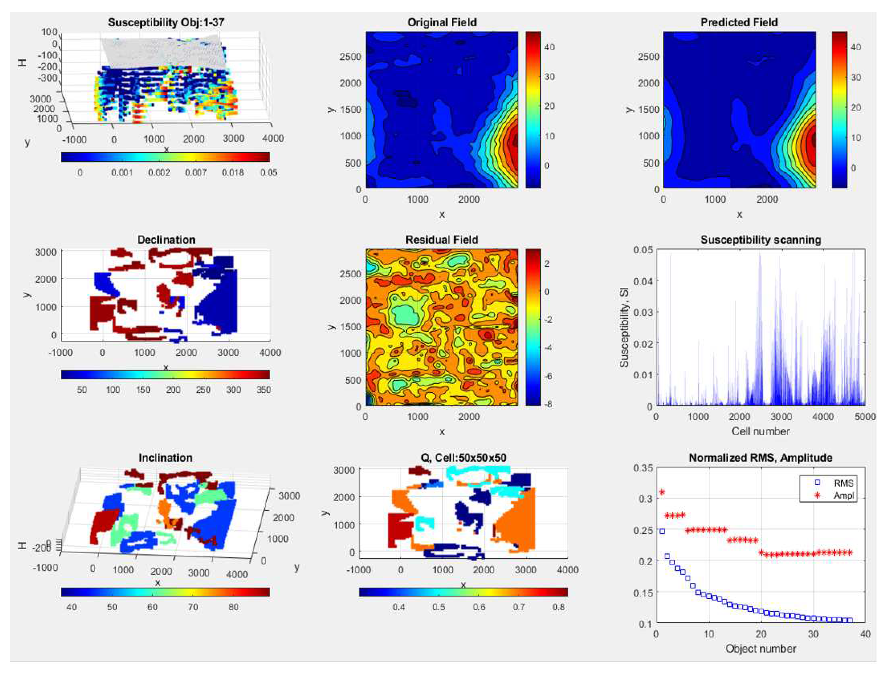
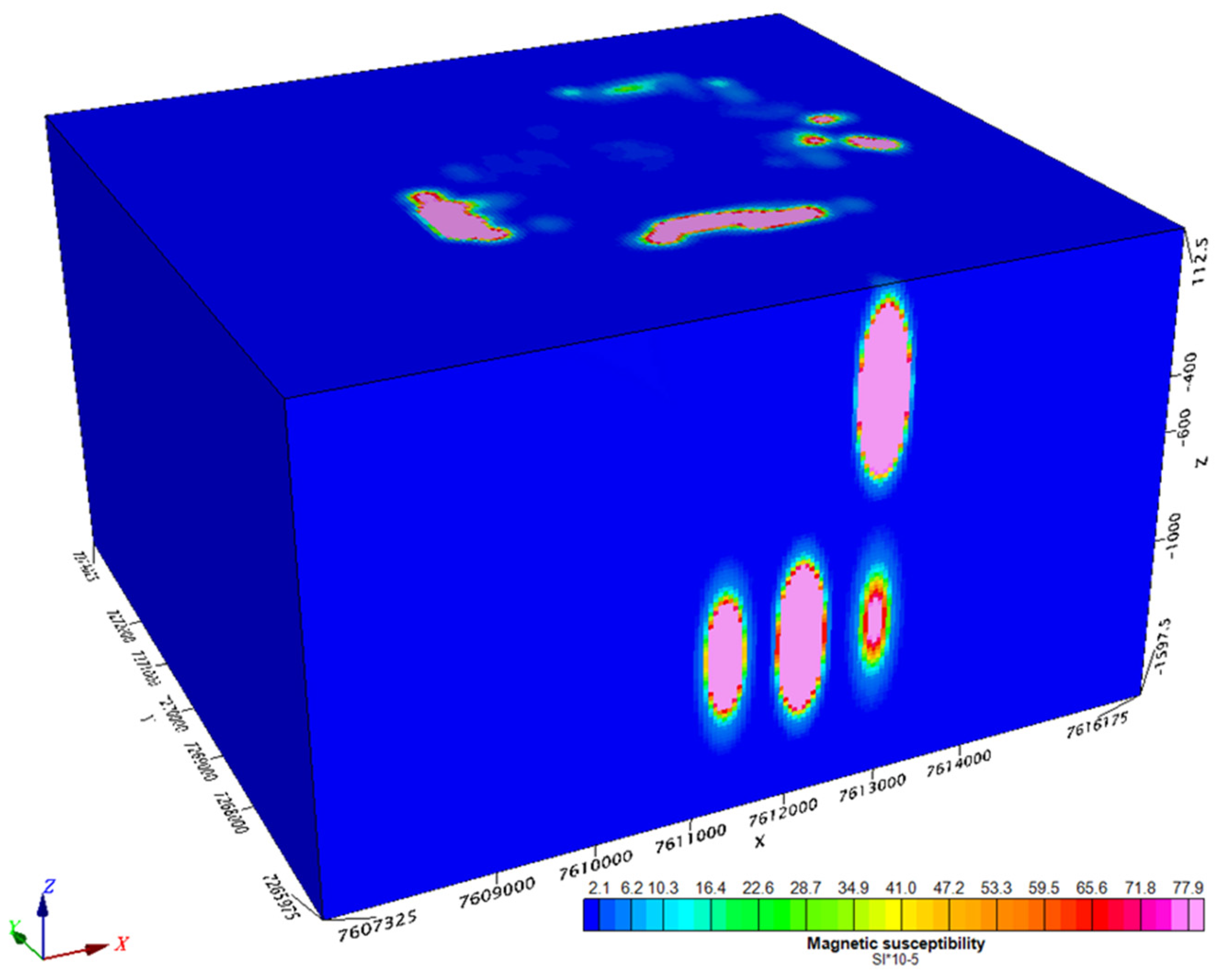
This algorithm was applied to the airborne magnetic data measured over Grib pipe. The starting mesh elements were set to 400 m in every direction and refined three times to 25 m. Figure 9 shows resulting model with all non-zero elements as well as data fit. A voxel model of magnetic susceptibility values was constructed from the QDIK inversion results (Figure 10).

4. Discussion

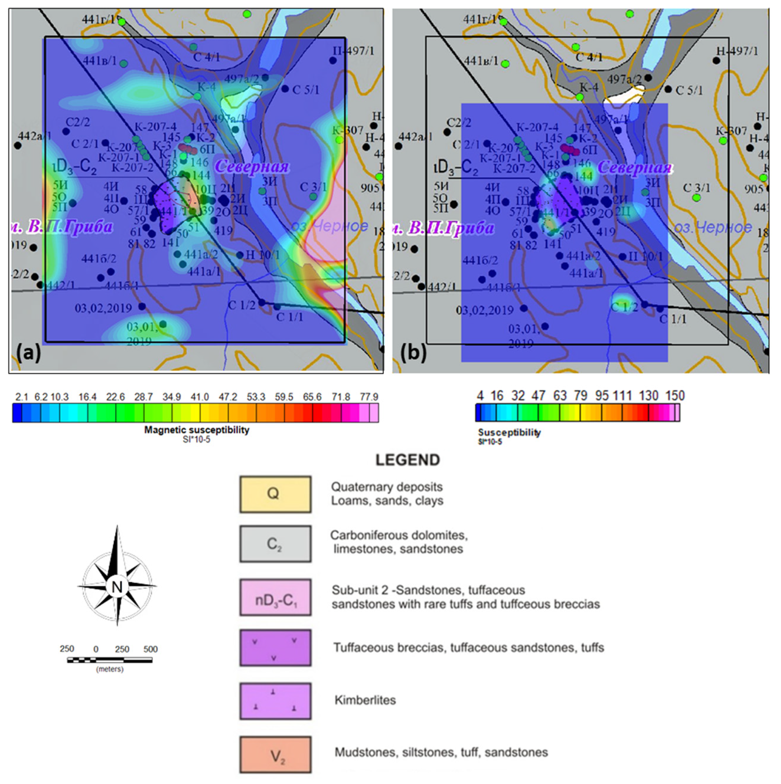
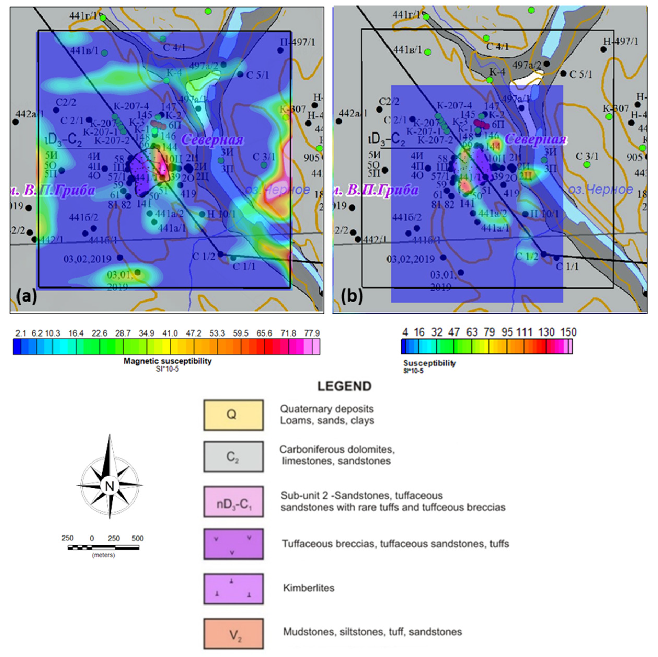
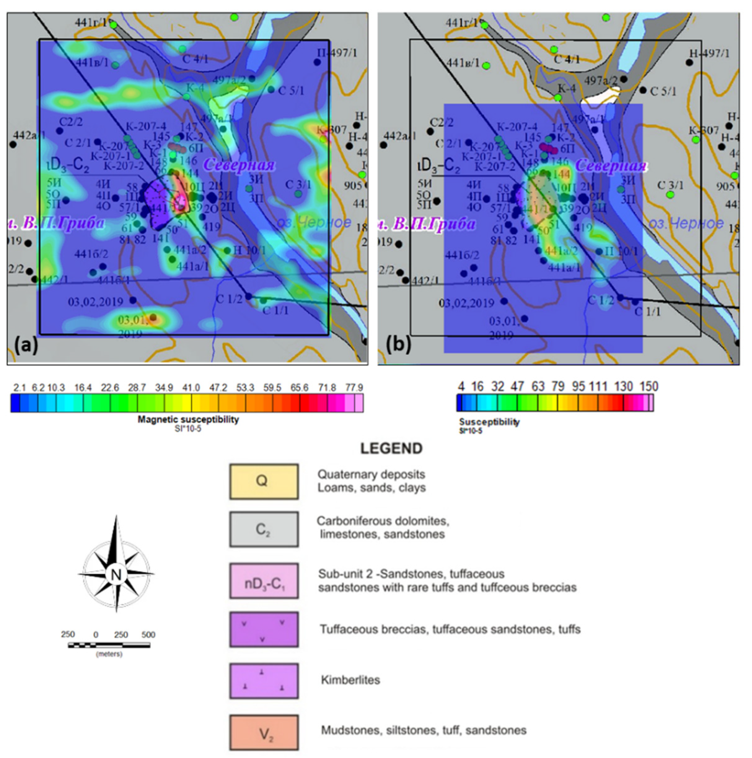
The results of two 3D inversion attempts are presented in a side by side comparison with known bedrock geology. Figure 11, Figure 12, Figure 13 and Figure 14 show plan view slices at different absolute elevations.

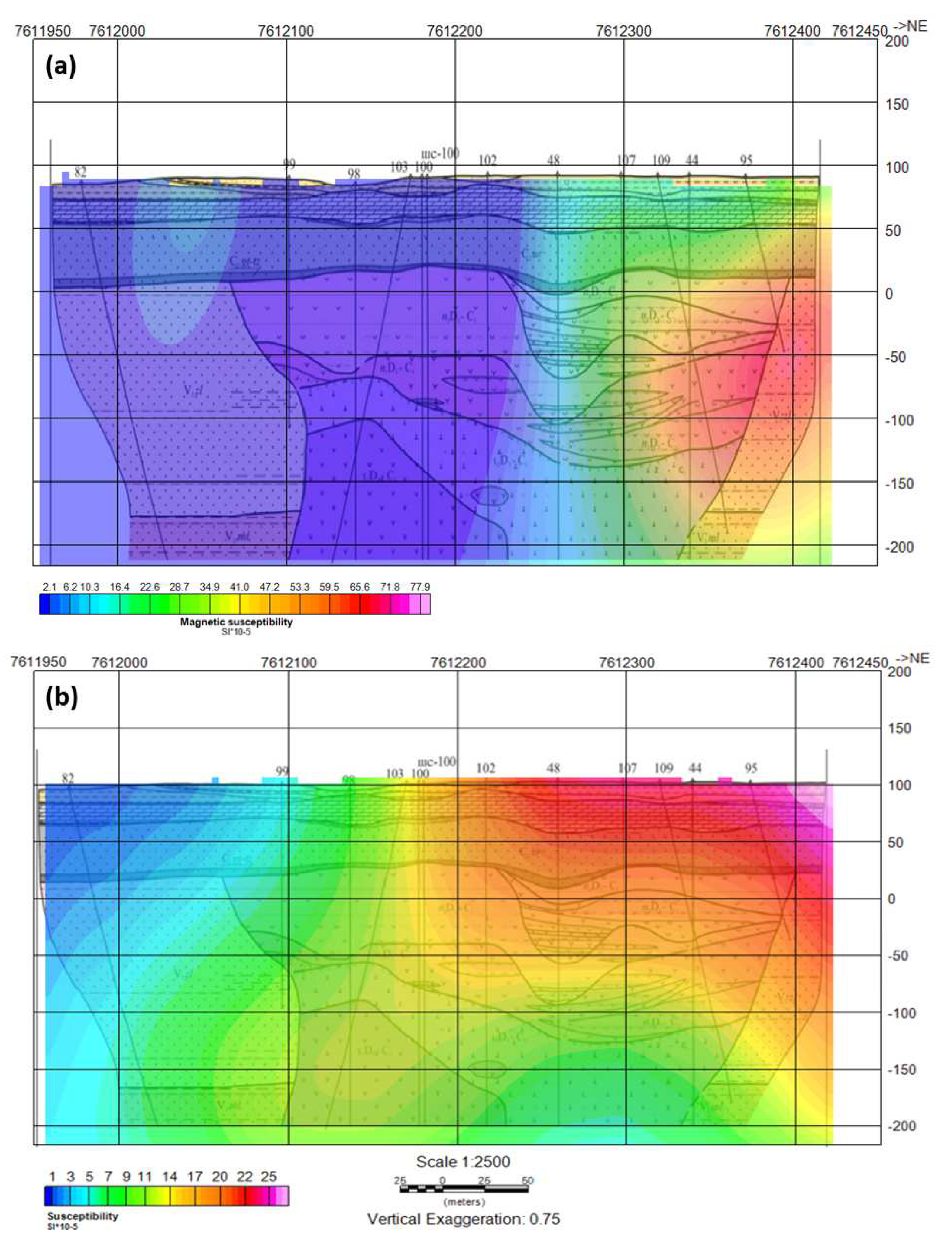
It becomes evident that both MVI and QDIK inversions show anomalous susceptibilities corresponding to pipe contours. The results are further examined in a cross-section. Figure 15 shows the AB geological cross-section over the Grib pipe. Figure 16 show sampled voxel models imposed over this cross-section (a): MVI inversion results and (b) QDIK inversion results.

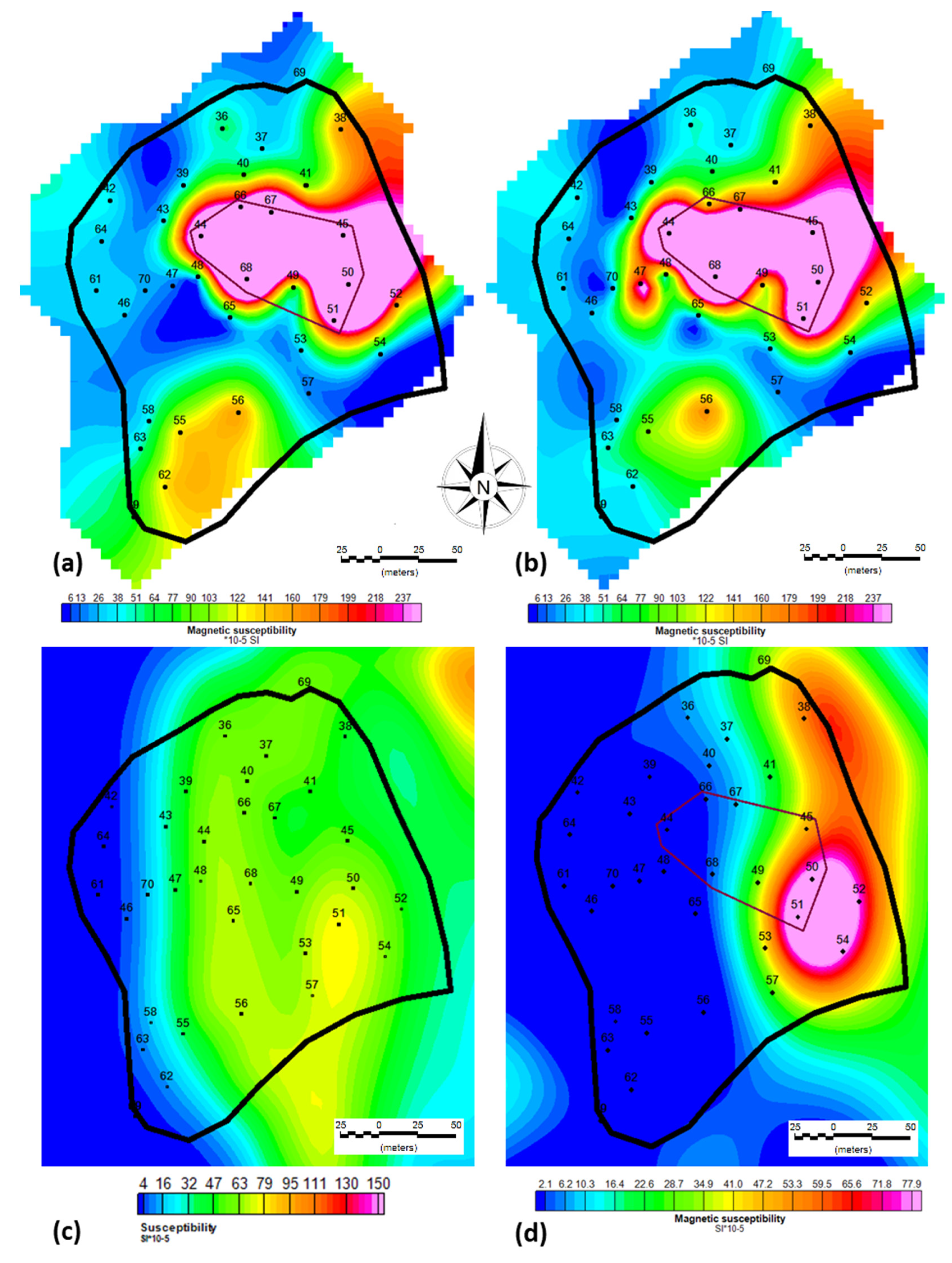
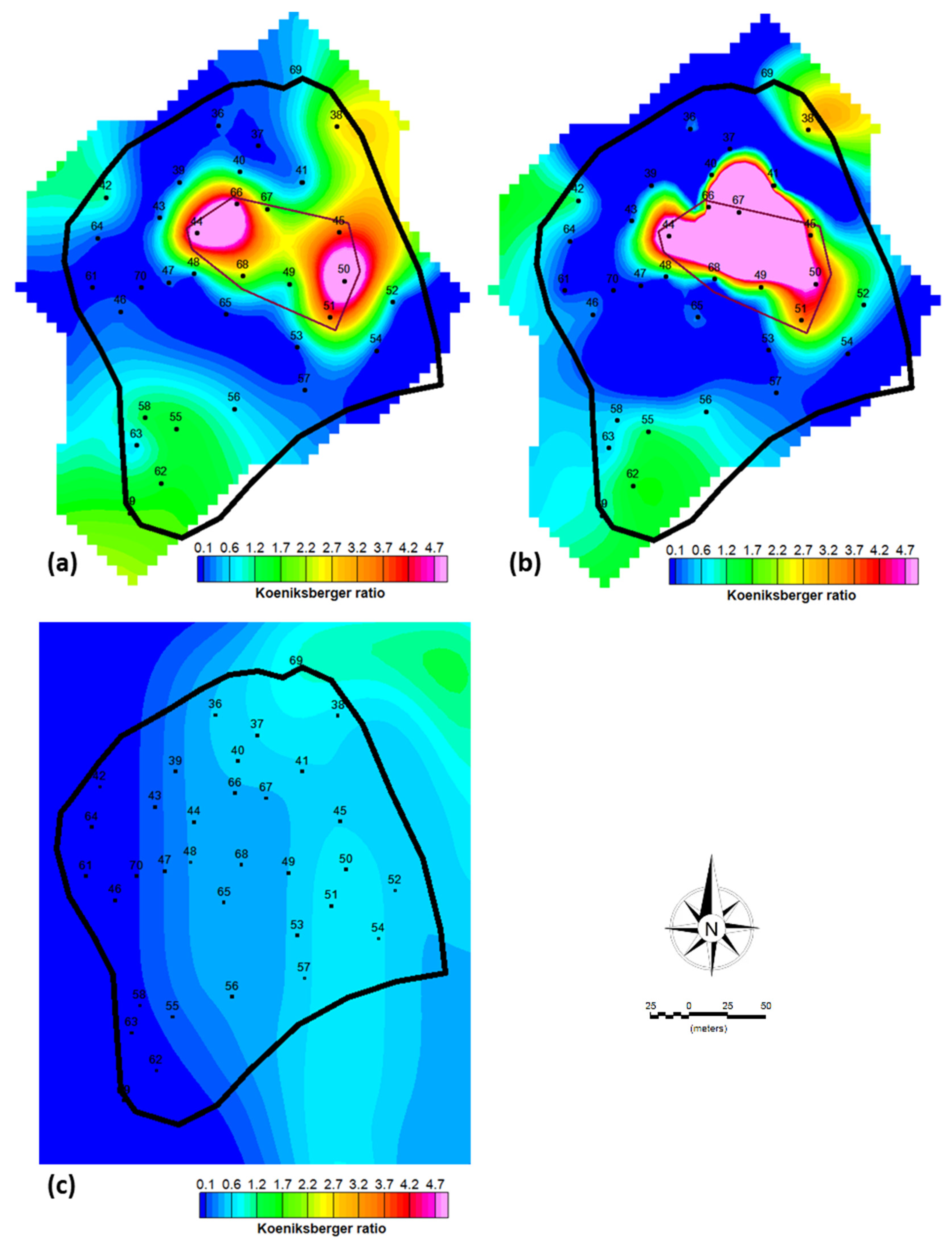
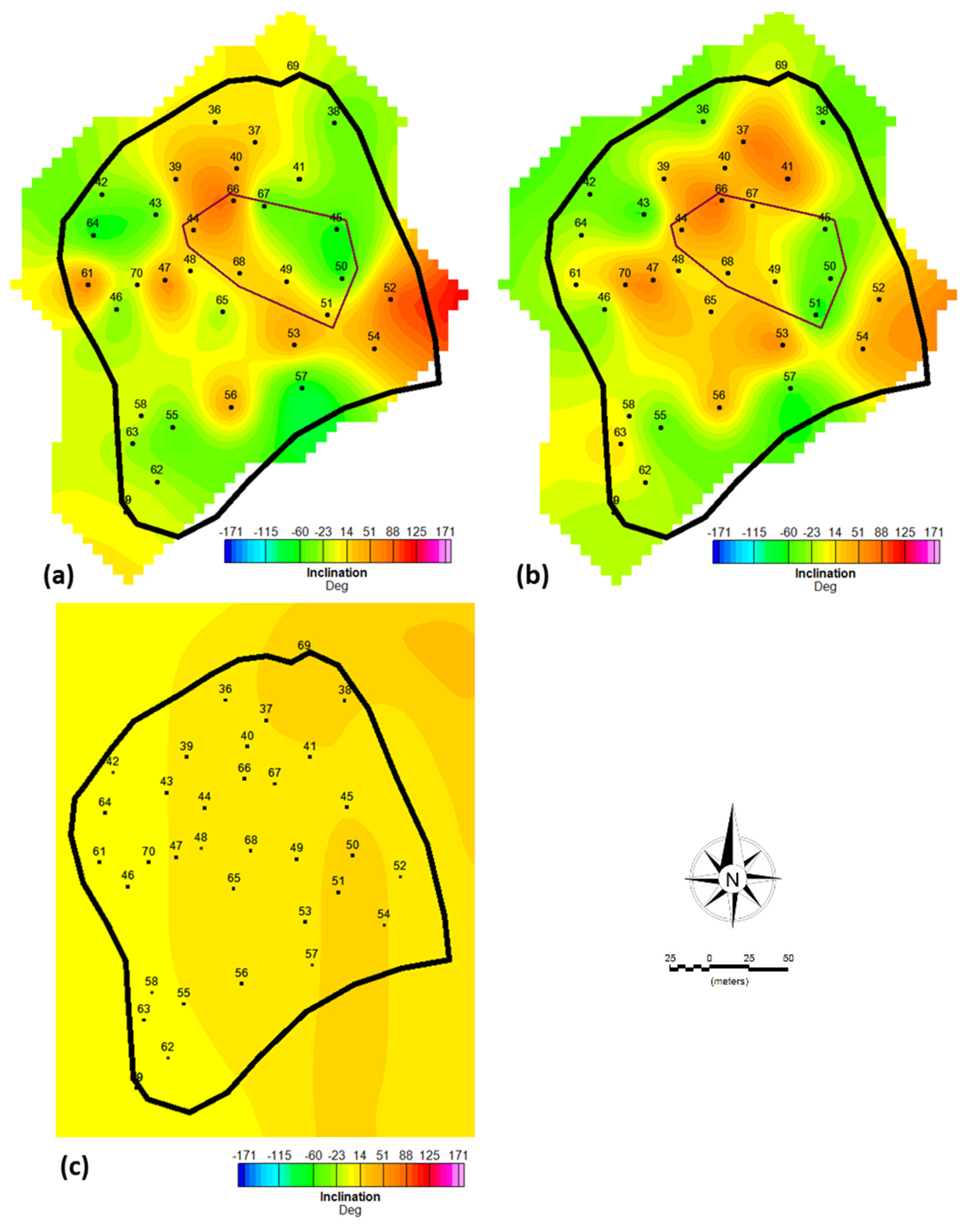
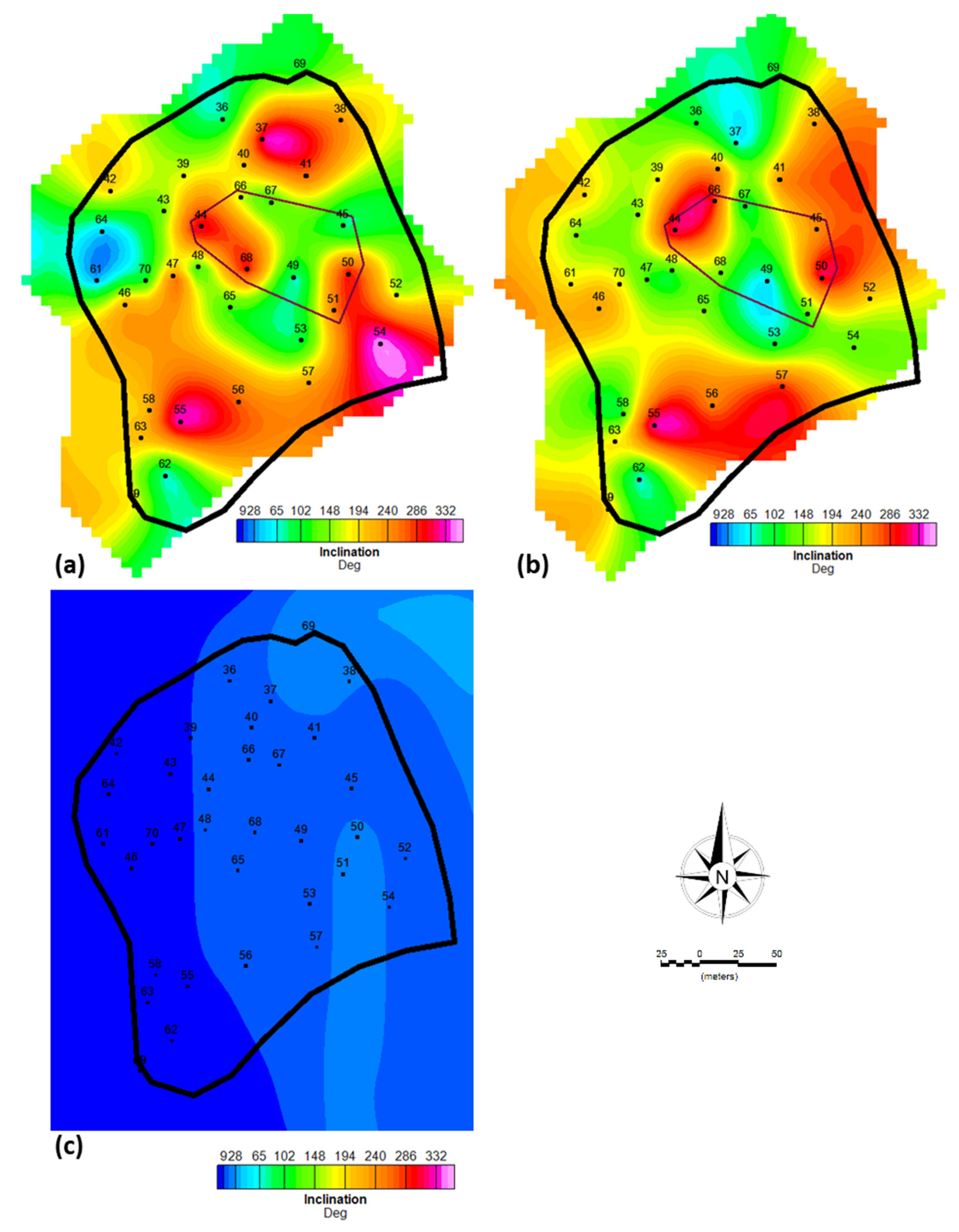
Finally, the result of the inversions were compared with the direct core petrophysical measurements. Figure 17, Figure 18, Figure 19 and Figure 20 show comparison of susceptibilities Koeniksberger ratios and values of remanent Inclination (I_r) and Declination (D_r). Voxel models presented in these figures were sliced at absolute elevation of 6 m, which corresponds to approximately 100 m depth (the upper part of the kimberlite pipe).

5. Conclusions

In current research we have demonstrated two different approaches to recover three-dimensional distribution of magnetic properties. It is evident that the MVI inversion yields smooth, yet confident recovery of the consolidated kimberlite units at depths starting at 100 m from surface (Figure 16), which is consistent with petrophysical studies. Furthermore, MVI approach allows noninvasive corrected magnetic susceptibility recovery from airborne data, which is at the same time somewhat consistent with susceptibilities uncovered by detailed sample petrophysical studies.

The QDIK inversion is quite complicated in terms of practical application however it provides interpretable results, including corrected susceptibility, Koeniksberger ratio and remanent magnetization vector parameters, all recovered non-invasively through analysis of remotely measured (airborne) data.

Comparing the two approaches, it can be concluded that MVI algorithm is more suitable for large-scale data sets and should be adapted as standard workflow in cases when remanent magnetization effects can not be neglected, while the QDIK algorithm is preferred on target-scale inverse modelling of non-invasive (airborne) data sets.

This study provides workflow for interpretation of both large and local airborne magnetic data sets, which is seen as a powerful tool in geological mapping, kimberlite exploration and the only algorithm existing to date to increase geophysical recovery of otherwise blind targets. It can be further combined with other remote sensing data sets to provide more effective target recovery.

Appendix A

Table A1. Scalar characteristics (J_n, K_m, mass) and direction of J_n for kimberlites and kimberlitic tuff breccias.

#	Sample	J_n A/m	K_m, SI units	Q	D°	I°	A₉₅	Mass (g)
1	2	3	4	5	6	7	8	9
Kimberlites
1	36-1	4.50E-03	5.98E-04	0.17	89	10.4	3.6	17.4
2	36-2	7.73E -03	4.83E-04	0.37	102.8	-32.4	0	16.4
3	37-1	1.65E-03	3.41E-04	0.11	334.1	17.4	4.3	16.7
4	37-2	1.09E-03	3.26E-04	0.08	57	69.3	0.2	16.7
5	38-1	1.91E-01	1.66E-03	2.64	237.1	-40.8	0.1	18.4
6	38-3	1.98E-01	1.58E-03	2.87	230.8	-42.5	0.2	18.8
7	39-1	2.07E-03	3.24E-04	0.15	173.5	31.8	1	16.5
8	39-2	2.03E-03	3.35E-04	0.14	174.5	29.9	0.4	15.8
9	40-1	1.43E-02	7.19E-04	0.46	207.2	37.3	4.8	17.8
10	40-2	6.07E-03	6.44E-04	0.22	241.5	19.4	0.2	18.1
11	41-1	1.41E-02	8.62E-04	0.38	265.5	-8.9	0.1	17.9
12	41-2	2.58E-02	1.19E-03	0.50	241.5	71.3	0	16.6
13	42-1	1.95E-02	4.19E-04	1.07	199	-32.6	1.7	17.2
14	42-2	2.09E-02	4.14E-04	1.16	199.8	-37.7	1.3	15.3
15	43-1	2.25E-03	3.05E-04	0.17	140.6	-48.2	3.1	16.8
16	43-2	3.32E-04	2.93E-04	0.03	144.3	-68.4	2.1	16.5
17	44-1	1.05E+00	3.82E-03	6.30	334.6	49.2	0.9	17.1
18	44-3	1.81E+00	5.45E-03	7.62	338.7	48.1	0.6	17.6
19	45-1	5.69E-01	3.37E-03	3.88	67	-63.7	0.5	18.1
20	45-2	4.24E-01	3.36E-03	2.90	239.8	-39.6	2.2	17.1
21	46-1	2.96E-03	2.76E-04	0.25	230.4	-38.6	1.4	16.5
22	46-2	4.58E-03	2.83E-04	0.37	235.3	-30.9	0.6	16.1
23	47-2	2.90E-03	2.38E-04	0.28	280.6	73.7	1.7	14.7
24	47-3	1.47E-02	3.15E-03	0.11	117.1	66.5	0.3	11.3
25	48-1	3.44E-03	2.74E-04	0.29	106.3	-6.8	1	15.9
26	48-2	2.30E-03	2.84E-04	0.19	113.9	4.6	0.2	15.9
27	49-1	1.49E-02	4.00E-04	0.85	58.5	12.3	0.8	16.7
28	49-2	7.95E-02	1.01E-03	1.80	47	11.7	3.3	17.7
29	50-1	1.98E+00	7.09E-03	6.40	307.6	-59.6	0.4	18.0
30	50-2	7.70E-01	3.54E-03	4.99	319.2	-44.4	2.2	17.4
31	51-1	4.86E-01	2.92E-03	3.81	259.3	14.2	3.8	15.8
32	51-2	6.03E-01	3.66E-03	3.78	123.6	-69	0.6	18.5
33	52-1	2.19E-02	1.49E-03	0.34	157.5	86	0.7	13.6
34	52-2	5.27E-02	1.31E-03	0.92	194.6	34.6	4.6	12.3
35	53-1	8.01E-04	2.97E-04	0.06	91.9	40.5	11	14.9
36	53-2	5.54E-04	2.93E-04	0.04	86.9	61.4	5.5	15.4
37	54-1	3.76E-04	2.63E-04	0.03	356.4	39.9	6.9	14.9
38	54-2	1.93E-04	2.56E-04	0.02	129.8	38.5	8	14.5
39	57-1	1.41E-03	1.56E-04	0.21	226.1	-81.9	6.8	12.7
40	57-2	1.41E-03	1.73E-04	0.19	289.6	-59.5	0	13.6
41	61-1	7.12E-04	3.07E-04	0.05	32.6	64.9	8.2	17.0
42	61-2	4.02E-04	2.87E-04	0.03	187.6	3.4	1.3	16.7
43	64-1	1.60E-03	2.77E-04	0.13	35.7	-70.1	1	15.2
44	64-2	1.33E-03	2.66E-04	0.11	144.2	-15.2	1.1	15.1
45	65-2	6.24E-04	2.73E-04	0.05	115.5	-20.9	11.7	15.1
46	65-3	4.29E-03	2.67E-04	0.37	147.3	17.4	4.9	15.0
47	66-1	6.32E-01	2.70E-03	5.37	161.6	74.9	0.7	16.9
48	66-2	1.17E-01	1.11E-03	2.41	297	80	4.6	16.0
49	67-1	3.35E-01	4.36E-03	1.76	113.5	-51.9	0.6	15.4
50	67-2	5.47E+00	2.47E-03	50.78	74	6.4	0.2	13.7
51	68-1	5.40E-01	5.46E-03	2.27	302.4	22.2	0.8	15.7
52	68-2	1.19E-01	5.95E-03	0.46	145.6	16.3	0.2	15.7
53	69-1	7.87E-03	3.14E-04	0.57	114.4	-0.5	0	12.4
54	69-3	1.67E-02	3.61E-04	1.06	110.7	-4.3	1.1	12.6
55	70-1	9.89E-05	2.36E-04	0.01	109.1	-3.5	3.2	14.2
56	70-2	9.24E-05	2.58E-04	0.01	181.8	55.4	2.8	15.3
57	Mean	2.80E-01	1.41E-03	Ji=43.6*1.41E-03=6.13E-02 А/м
Kimberlitic tuff breccias
58	55-2	8.11E-02	1.32E-03	1.41	329.5	-44.1	2.8	15.3
59	55-4	5.26E-02	1.01E-03	1.20	321.1	-41.3	0.3	14.2
60	56-1	5.07E-02	1.61E-03	0.72	269.1	42.5	0.2	13.5
61	56-2	5.96E-02	1.71E-03	0.80	253.1	34.3	4.2	11.8
62	58-1	2.30E-02	4.16E-04	1.27	215.4	-9.9	0.1	12.1
63	58-2	8.00E-03	2.60E-04	0.71	110.8	-7.1	3.6	11.2
64	59-1	1.88E-02	5.58E-04	0.77	142.2	-35.2	0.5	16.5
65	59-2	1.52E-02	5.26E-04	0.66	191.1	-43.1	0.5	16.0
66	60-1	1.02E-01	9.01E-04	2.60	228.6	27	5.2	13.9
67	60-2	1.24E-02	2.23E-04	1.27	221.1	5.4	0.1	12.6
68	62-1	9.00E-02	1.36E-03	1.51	58.2	-19.1	1.8	12.5
69	62-2	2.50E-02	3.68E-04	1.56	54.2	-11.8	2.5	14.7
70	63-1	1.36E-02	4.75E-04	0.66	215.1	-26.9	4.5	14.0
71	63-2	1.36E-02	5.19E-04	0.60	197.3	11.9	4.1	14.2
72	Mean	4.04E-02	8.04E-04	Ji=43.6*8.04E-04=3.51E-02 А/м
73	Mean (all rock types)	2.32E-01	1.29E-03	Ji=43.6*1.29E-03=5.61E-02 А/м

References

Pendelyak, R.N.; Verichev, E.M.; Golovin, N.N. Grib deposit: Geological structure and diamond content. Minig Journal 2014, 16–21. [Google Scholar]
Arnautov, A.I.; Iskhakov, M.S. Engineering and environmental problems in the development of the V.P. Grib diamond deposit. Notes of the Mining Institute 2003, 153, 117–119. (In Russian) [Google Scholar]
Kjarsgaard, B.A. Kimberlite pipe models: Significance for exploration; In: B. Milkereit (Ed.), Proceedings of Exploration 07: Fifth Decennial nternational Conference on Mineral Exploration, 2007, np. 667-677.
Dmitrieva, T.N. Petrophysical and paleomagnetic research of rocks composing the Grib kimberlite pipe. Technical report 2021, 58. [Google Scholar]
Ellis, R.G.; Wet, B.; Macleod, I.N. Inversion of Magnetic Data from Remanent and Induced Sources. ASEG Extended Abstracts 2012, 1, 1–4. [Google Scholar] [CrossRef]
Davydenko A.Y. Inversion of magnetic field based on elastic meshes аnd vector scanning for evaluation of magnetic susceptibility and remanent mаgnetization of 3D objects. Рproceedings of meeting: Theory and practice of geological interpretation of geophysical fields, 47-th session of International seminar, Voronezh, 2020; pp. 105–110. (In Russian).
Telford, W.M.; Geldart, L.P.; Sheriff, R.E.; et al. Applied geophysics, 2nd ed.; Cambridge university press, 1990; p. 622. ISBN 0-521-32693-1. [Google Scholar]
Clark, D.A. Methods for determining remanent and total magnetizations of magnetic sources – a review. Journal of applied geophysics 2014, 45, 271–304. [Google Scholar]
Li, Y.; Shearer, S.E.; Haney M., M.; Dannemiller, N. Comprehensive approach to 3D inversion of magnetic data affected by remanent magnetization. Journal of geophysics 2010, 75, L1–L11. [Google Scholar] [CrossRef]
Zou, H.; Hastie, T. Regularization and Variable Selection via the Elastic Net. Journal of the Royal Statistical Society B 2005, 67, 301–320. [Google Scholar] [CrossRef]

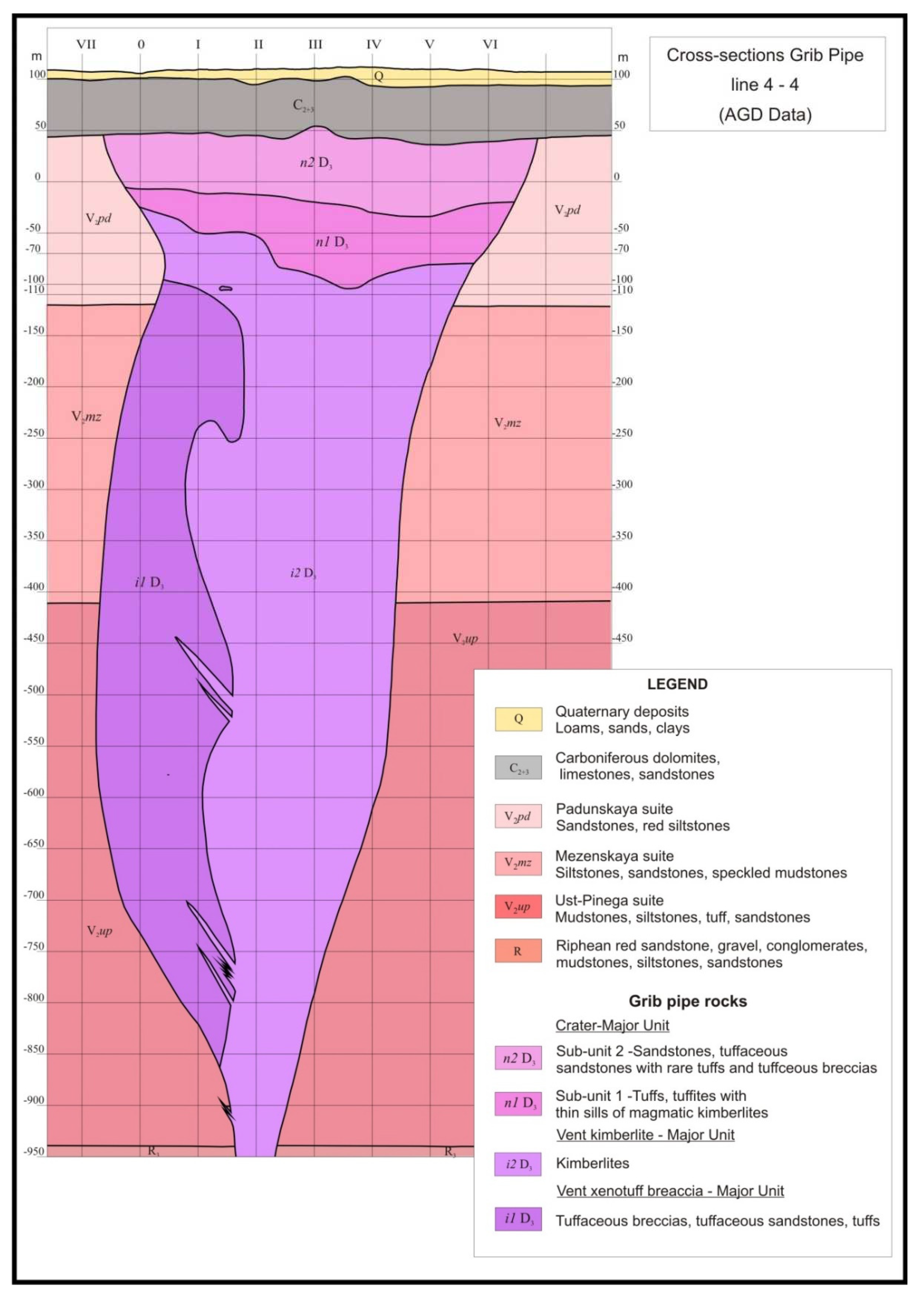
Figure 1. The cross-section of Grib kimberlite pipe [1].

Figure 2. Distribution histograms of Jn and Km of Grib pipe kimberlite rocks.

Figure 3. Relationships between Jn and Km of Grib pipe kimberlite rocks.

Figure 4. Sample collection map. Red markings indicate most recent sampling used for petrophysical studies.

Figure 5. (a) Residual Magnetic Field plotted over bedrock geology of Grib pipe. Flight lines (E-W) are shown in black. (b) Residual Magnetic Field plotted over bedrock geology of Grib pipe after trend removal.

Figure 6. Magnetic susceptibility derived from the MVI inversion.

Figure 7. Magnetization vector voxel model, derived from the MVI inversion.

Figure 8. Data fit for the MVI inversion. (a) Observed TMI. (b) Predicted TMI.

Figure 9. Data fit and results for QDIK inversion (50 m mesh).

Figure 10. Calculated magnetic susceptibility voxel model derived from QDIK inversion.

Figure 11. Slices of magnetic susceptibilities at -200 m abs. elevation derived from (a): MVI inversion. (b) QDIK inversion. (c): conventional scalar inversion.

Figure 12. Slices of magnetic susceptibilities at -100 m abs. elevation derived from (a): MVI inversion. (b) QDIK inversion. (c): conventional scalar inversion.

Figure 13. Slices of magnetic susceptibilities at 0 m abs. elevation derived from (a): MVI inversion. (b) QDIK inversion. (c): conventional scalar inversion.

Figure 14. Slices of magnetic susceptibilities at 50 m abs. elevation derived from (a): MVI inversion. (b) QDIK inversion. (c): conventional scalar inversion.

Figure 15. Geological cross-section AB over Grib pipe.

Figure 16. (a) Results of MVI inversion sampled over the AB cross-section. (b). Results of QDIK inversion sampled over the AB cross-section.

Figure 17. Magnetic susceptibility derived from (a): Sample collection 1. (b): Sample collection 2. (c) QDIK inversion (6m abs. elevation). (d): MVI inversion (6m abs. elevation).

Figure 18. Koeniksberger ratio derived from (a): Sample collection 1. (b): Sample collection 2. (c) QDIK inversion (6m abs. elevation).

Figure 19. Remanent Inclination (Ir) derived from (a): Sample collection 1. (b): Sample collection 2. (c) QDIK inversion (6m abs. elevation).

Figure 20. Remanent declination (Dr) derived from (a): Sample collection 1. (b): Sample collection 2. (c) QDIK inversion (6m abs. elevation).

Table 1. Mean values of rock type scalars (Jn, Km).

#	Rock types	Number of samples	Range of Jn, A/m		Mean values Jn, A/m	Range of Km, SI units		Average values of Km, SI units
1	Kimberlites	56	min	max	1.29E-04	min	max	1.41E-03
1	Kimberlites	56	9.24E-05	5.47E+00	(2.80E-01)	1.56E-04	7.09E -03	(7.18E-04)
2	Kimberlitic tuff breccias	14	min	max	2.94E-02	min	max	6.59E-04
2	Kimberlitic tuff breccias	14	8.00E-03	1.02E-01	(4.04E-02)	1.23E-04	1.71E-03	(8.04E-04)
3	All rock types	70	min	max	1.52 E-02	min	max	7.05E -04
3	All rock types	70	9.24E-05	5.47E+00	(2.32E-01)	1.56E-04	7.09E -03	(1.29E-03)

Table 2. Magnetic properties of host rocks around Grib kimberlite pipe.

Age	Rock type	Magnetic susceptibility (x10^-5 SI units)	Magnetic susceptibility (x10^-5 SI units averaged)	Remanent magnetization (x10^-3 A/m)
V₂zl (Zolotnickaya suite)	Sandstones	0-36	28.65	0-185
	Coarse-grained sandstones	0-11	8.75	1-58
	Iron sandstones	5-1182	940.63	4-413
	Silts	1-80	63.66	1-29
	Argillites	10-100	79.58	5.6-60
V₂ml (Melskaya suite)	Sandstones	1-36	28.65	0.6-11.7
	Silts	1-28	22.28	0.3-11
	Iron sandstones	21-26	20.69	11
V₂er (Erginskaya suite)	Sandstones	2-31	24.67	0.6-6.9
	Silts	10-28	22.28	0.7-11
	Argillites	14-39	31.04	5.5-6.9
V₂up (Ust-pinejskaya suite)	Sandstones	3-226	179.85	0.5

Disclaimer/Publisher’s Note: The statements, opinions and data contained in all publications are solely those of the individual author(s) and contributor(s) and not of MDPI and/or the editor(s). MDPI and/or the editor(s) disclaim responsibility for any injury to people or property resulting from any ideas, methods, instructions or products referred to in the content.

© 2023 by the authors. Licensee MDPI, Basel, Switzerland. This article is an open access article distributed under the terms and conditions of the Creative Commons Attribution (CC BY) license (http://creativecommons.org/licenses/by/4.0/).

Copyright: This open access article is published under a Creative Commons CC BY 4.0 license, which permit the free download, distribution, and reuse, provided that the author and preprint are cited in any reuse.

MDPI Initiatives

Important Links

Choose an area of interest and we will send you notifications of new preprints at your preferred frequency.

Disclaimer

Geological Mapping of Grib Kimberlite Pipe Using 3D Magnetization Vector Inversion From Airborne Data

Abstract

1. Introduction

1.1. Geology

1.2. Magnetic properties

2. Materials and Methods

3. Results

3.1. MVI inversion

3.2. QDIK inversion

4. Discussion

5. Conclusions

Appendix A

References

MDPI Initiatives

Important Links

Subscribe