Preprint

Article

Low-Cost Denoising and Deblurring Using a Novel Nonlinear Diffusion Technique

Altmetrics

Downloads

113

Views

Comments

This version is not peer-reviewed

Submitted:

09 June 2023

Posted:

12 June 2023

You are already at the latest version

Alerts

Abstract

An algorithm for the treatment of images affected by both blurring and salt&pepper noise is proposed with a cost only proportional to the number of pixels. The methodology uses a discretization scheme for the Laplace operator multiplied by a suitable nonlinear term depending on the gradient. Even if this approach resembles a diffusion type algorithm, only one step of the procedure is applied, leading to significant time savings. The procedure is successfully tested on some standard black&white natural images.

Keywords:

Subject: Computer Science and Mathematics - Computer Vision and Graphics

1. Introduction

An image, both in the acquisition and transmission phase, can be affected by various types of noise. In the field of image processing, noise refers to (random) variations in the signal that affect information extraction. We consider here some classical examples of image noise. Blurring is quite typical and happens, for example, when the recording is out of focus. Salt&pepper noise contaminates instead an image randomly, by converting some pixel values into white or black dots. The causes generating these type of disturbances can be rather different and are well known to those working in the field of two- or three-dimensional images. Restoration is therefore necessary in the most desperate cases and the current literature is able to propose numerous remedies.

The variety of image noise reduction methods that have been developed include, among others: filter methods, wavelet methods, diffusion methods, total variation methods, sparse representation methods, Markov random field models, and, especially in recent years, Artificial Intelligence (AI) methods. To get a quick overview of the field, we refer the interested reader to the following (non-exhaustive) selection of articles and reference books: [1,2,3,4,5,6,7,8,9,10,11,12,13,14,15,16,17,18,19,20,21].

Filter-based methods, like Gaussian or median filters, are simple and computationally efficient techniques for reducing noise. These filters help smooth out random variations in pixel values caused by noise, resulting in a cleaner image. In addition, advanced noise reduction algorithms, such as wavelet or total variation denoising, can be used to effectively reduce disturbances while preserving image detail. Unfortunately, basic filters can result in a loss of detail, while advanced denoising algorithms are more computationally demanding. Moreover, strict tuning of parameters is often required for optimal performance.

To deal with blurring, different techniques can be employed based on the specific blur characteristics. Some algorithms, such as Wiener’s or blind deconvolution, aim to reverse the blurring effect and can potentially recover sharp detail in the image. Though some recent algorithms can be used without prior knowledge, deconvolution methods can be sensitive to noise and can amplify it in the process. Furthermore, accurate parameter estimation can be challenging in real-world scenarios.

AI-based deblurring and denoising techniques have shown promise in image processing. These techniques use deep learning models, such as Convolutional Neural Networks (CNNs), to learn the mapping between blurry/noisy images and their corresponding clean versions. AI-powered deblurring and denoising techniques have demonstrated significant improvements over traditional methods. They can handle complex noise patterns and capture intricate image detail. However, these techniques require large amounts of training data, computational resources, and careful model selection and parameter tuning in order to achieve optimal results.

Overall, the selection of appropriate approaches to denoising and deblurring depends on several factors, such as the specific characteristics of the image, the level of noise or blurring, and the desired outcome. This often involves a trade-off between noise reduction and preservation of the details. To conclude, while image denoising is an established and extensively studied problem, it remains a challenging and open task. The main reason for this is that, mathematically speaking, image denoising is an ill-posed inverse problem with a non-unique solution.

Among the various mathematical approaches, variational and Partial Differential Equations (PDEs) based methods have played a crucial role in the progress of image processing, specifically in the areas of denoising and deblurring. Starting from the pioneering works of Mumford-Shah [22] and Perona-Malik [1], image denoising using nonlinear or anisotropic diffusion, closely connected with variational methods, is a commonly used technique (see, e.g., [14,20] and the references therein). In addition, for salt&pepper noise, median filtering, first proposed by Tukey [23], is still widely regarded as an effective processing technique. The value at each pixel is substituted by the median of the values at the surrounding points. This leads to the unfortunate result of adding blur, thereby weakening the image features. Techniques such as neighborhood or Gaussian filtering also have similar drawbacks. If such blur was already present in the original image the outcome can be disastrous. On the other hand, the treatment of blurring can turn out to be quite expensive.

In this paper we take into consideration a recent methodology based on a diffusion PDE as introduced in [24,25], which allows us to preserve the fundamental shapes of the image during the denoising phase. The technique has been successfully applied in the field of edge-detection and partially used to treat some images affected by blur. Here we extend our experimental analysis to images that are both blurred and contaminated by salt&pepper noise, confirming that the approach can give good results at a rather low cost. The technique is partially included among those that are classified as "nonlinear diffusion", where a certain number of steps are applied to the figure with the aim of homogenizing the areas of slight variation and instead emphasizing the contours. In our case the PDE under consideration is:

\frac{\partial u}{\partial t} = \sqrt{\frac{{∥ \nabla u ∥}^{2}}{1 + {∥ \nabla u ∥}^{2}}} Δ u,

(1)

where ∇ denotes the gradient and

Δ

is the Laplace operator. The function u is built on the values of the image under consideration via the classical equispaced grid. The equation is defined on a rectangle where Neumann conditions are imposed on the boundaries. Thus, the nonlinear diffusion coefficient depends locally on the magnitude of the gradient. Equation (1) differs substantially from those generally considered in the scientific literature. Moreover, as explained in [24], the differential operator is approximated by means of a high-order finite difference scheme. The residuals are calculated on a staggered grid and subsequently interpolated on the standard grid. In order not to burden the discussion here, the details of the construction are given in Section 2.

To clarify the reasons for our approach, we show in Section 3 some results in one dimension (1D), where the function u is only affected by salt&pepper noise. In Section 4, we generalize these results to two-dimensional (2D) images that are simultaneously disturbed by blur and noise. As the reader will see, by only a couple of steps of the algorithm, we will be able to reconstruct the corrupted images quite faithfully. The cost of this restoration will be of the same order as the number of pixels that make up the figure. This ensures a substantial cost reduction compared to other algorithms already in use.

2. Construction of the Algorithm

We describe here the procedure for calculating the discrete derivatives in order to build the discretization of the nonlinear differential operator in (1). We have a first grid made up of points

(x_{i}, y_{j})

, where the pixel values

u_{i, j}

of the figure to be treated are stored. The points are equally spaced and in the two directions their distance is equal to h, that is

x_{i + 1} = x_{i} + h, y_{j + 1} = y_{j} + h, i, j = 0, 1, \dots N,

(2)

where N denotes the number of pixels along a given direction. Without this constituting a restriction, we will take

h = 1

in our 2D calculations. Moreover, for simplicity, we omit to specify the range of variability of the indices.

An intermediate grid

(x_{i + 1 / 2}, y_{j + 1 / 2})

built on half-fractional indices (otherwise called "staggered grid") is also taken into consideration, where

\begin{matrix} x_{i + 1 / 2} = x_{i} + \frac{h}{2}, y_{j + 1 / 2} = y_{j} + \frac{h}{2} . \end{matrix}

(3)

In order to enforce Neumann conditions, a couple of extra (fictitious) layers outside the grid boundary are introduced.

From the original values

u_{i, j}

, we define new values at the shifted nodes according to:

\begin{matrix} u_{i + 3 / 2, j + 1} = \frac{1}{2} (u_{i + 1, j + 1} + u_{i + 2, j + 1}), \end{matrix}

(4)

\begin{matrix} u_{i + 1, j + 3 / 2} = \frac{1}{2} (u_{i + 1, j + 1} + u_{i + 1, j + 2}), \end{matrix}

(5)

so that we can build the following discrete partial derivatives:

\begin{matrix} d_{i + 3 / 2, j + 3 / 2}^{x} = \frac{1}{h} (u_{i + 2, j + 3 / 2} - u_{i + 1, j + 3 / 2}), \end{matrix}

(6)

\begin{matrix} d_{i + 3 / 2, j + 3 / 2}^{y} = \frac{1}{h} (u_{i + 3 / 2, j + 2} - u_{i + 3 / 2, j + 1}) . \end{matrix}

(7)

As a consequence, the Laplace operator at the staggered grid points takes the expression:

\begin{matrix} l_{i + 3 / 2, j + 3 / 2} & = & \frac{1}{2 h} (d_{i + 5 / 2, j + 3 / 2}^{x} - d_{i + 1 / 2, j + 3 / 2}^{x} + d_{i + 3 / 2, j + 5 / 2}^{y} - d_{i + 3 / 2, j + 1 / 2}^{y}) \\ \approx & (Δ u) (x_{i + 3 / 2, j + 3 / 2}) . \end{matrix}

(8)

Successively, we write:

\begin{matrix} R_{i + 3 / 2, j + 3 / 2} = {(\frac{{(D_{i + 3 / 2, j + 3 / 2})}^{2}}{1 + {(D_{i + 3 / 2, j + 3 / 2})}^{2}})}^{1 / 2} l_{i + 3 / 2, j + 3 / 2}, \end{matrix}

(9)

where

\begin{matrix} D_{i + 3 / 2, j + 3 / 2} = {({(d_{i + 3 / 2, j + 3 / 2}^{x})}^{2} + {(d_{i + 3 / 2, j + 3 / 2}^{y})}^{2})}^{1 / 2} . \end{matrix}

(10)

The final step is to interpolate the values (9) from the staggered to the integer grid. To this end, we apply the following formula:

\begin{matrix} R_{i, j} & \approx & \frac{1}{256} (R_{i - 3 / 2, j - 3 / 2} - 9 R_{i - 3 / 2, j - 1 / 2} - 9 R_{i - 3 / 2, j + 1 / 2} + R_{i - 3 / 2, j + 3 / 2} - 9 R_{i - 1 / 2, j - 3 / 2} \\ + 81 R_{i - 1 / 2, j - 1 / 2} + 81 R_{i - 1 / 2, j + 1 / 2} - 9 R_{i - 1 / 2, j + 3 / 2} - 9 R_{i - 1 / 2, j + 3 / 2} - 9 R_{i + 1 / 2, j - 3 / 2} \\ + 81 R_{i + 1 / 2, j - 1 / 2} + 81 R_{i + 1 / 2, j + 1 / 2} - 9 R_{i + 1 / 2, j + 3 / 2} + R_{i + 3 / 2, j - 3 / 2} - 9 R_{i + 3 / 2, j - 1 / 2} \\ - 9 R_{i + 3 / 2, j + 1 / 2} + R_{i + 3 / 2, j + 3 / 2}) . \end{matrix}

(11)

All the above operations are quite accurate, since it turns out that the formulas are exact up to polynomials of degree three.

A time-discretization algorithm for (1) is obtained through the following step:

u_{i, j} \leftarrow u_{i, j} + γ R_{i, j},

(12)

where

γ \in R

is a suitable parameter that can be either taken positive or negative. A complete approximation in time would require several steps of (12). However, in all the applications that will be considered it is sufficient to make a single iteration to get more than satisfactory results. In this case the choice of

γ

is crucial.

To conclude, the proposed algorithm can be summarized by the following passages:

Algorithm 1

Consider the original image given by the values $u_{i, j}$ at the points $(x_{i}, y_{j})$ ;
Build the centered discretization (9) of the nonlinear space operator in (1) at the staggered grid points;
By polynomial interpolation, pass from the staggered to the classical grid, evaluating the quantities $R_{i, j}$ in (11);
Update the image using (12);
Reiterate if necessary.

Further clarifications and suggestions regarding the algorithm are provided in [24]. Here we only observe that a single iteration of the algorithm is already capable of enhancing object contour lines or sharpening blurred images. As a result, this procedure can effectively be applied in edge detection or denoising techniques, either independently or in combination with established methods. Although possible, it is not recommended to apply the method for multiple iterations, as there is a risk of worsening the result instead of improving it, introducing unwanted oscillations along the edges.

In this paper we use the algorithm for image denoising and deblurring, but the versatility of proposed method extends beyond these domains, making it valuable for image enhancement, object segmentation, and data analysis. With its ability to deliver accurate and high-quality results, this algorithm may constitute a powerful tool in the field of computer vision and image processing.

3. Treatment of Salt&Pepper in 1D

For simplicity, we start by first showing our denoising algorithm in a one-dimensional case. The operator to be discretized assumes the following form:

\sqrt{\frac{{(\partial u / \partial x)}^{2}}{1 + {(\partial u / \partial x)}^{2}}} \frac{\partial^{2} u}{\partial x^{2}},

(13)

and it is applied to u defined on a finite interval. This is the one-dimensional version of the operator in (1) as also made explicit in [24]. The problem is supplied with boundary constraints of Neumann type at the extremes of the interval. Now N is the number of pixels

x_{i + 1} = x_{i} + h

i = 1, 2, \dots, N

, and the image is represented by the values

u_{i}

belonging to a palette with tones of grey from black (level 0) to white (level 1). In particular, in our example, we will recover such values from the function

u (x) = \frac{1}{2} (1 + sin (7 π x))

x \in [0, 1]

. We take

N = 100

and

h = 1 / N

We modify the function at randomly chosen points setting the values to 0 or 1 (salt&pepper noise). In the left plots of Figure 1 and Figure 2, the new function is visible where the change was made in 10 or 50 points, respectively. The discrete version of the operator (1) is applied to the vector

u_{i}

, so obtaining a new vector

R_{i}

. This means that we first have to compute the derivatives in the staggered grid and then re-interpolate everything to the standard grid. The results after this procedure are illustrated in the central plots of Figure 1 and Figure 2. It is evident that, in the presence of the discontinuities of u, the operator presents pronounced peaks. These are a symptom of the presence of salt&pepper grains in the original function. At this point we can introduce a cutoff parameter

τ > 0

and modify the values that are above the threshold. This is done by replacing the corresponding value of u with the median of the values surrounding it. The calculation is as follows:

u_{i}^{*} = \frac{1}{2} (u_{i - 1} + u_{i + 1}) only if | R_{i} | \geq τ .

(14)

No correction is made at the other points. The denoised signals

u_{i}^{*}

is shown in the last plots of Figure 1 and Figure 2, and corresponds to the choice

τ = \frac{1}{2} (| R_{i - 1} | + | R_{i + 1} |)

Figure 1. The original function modified at 10 points (left), the corresponding plot of the vector

R_{i}

(centre), the function after correction (right).

Figure 1. The original function modified at 10 points (left), the corresponding plot of the vector

R_{i}

(centre), the function after correction (right).

Figure 2. The original function modified at 50 points (left), the corresponding plot of the vector

R_{i}

(centre), the function after correction (right). Here some values have not been replaced since the corresponding points of noise were consecutive, producing an ambiguous behavior of the values

R_{i}

Figure 2. The original function modified at 50 points (left), the corresponding plot of the vector

R_{i}

(centre), the function after correction (right). Here some values have not been replaced since the corresponding points of noise were consecutive, producing an ambiguous behavior of the values

R_{i}

The reconstruction is not always perfect. It certainly depends on the choice of the parameter

τ

, but also on the fact that when there are two consecutive grains of the type salt&salt, salt&pepper or pepper&pepper, the vector

R_{i}

does not provide reliable indications. However, the advantage is applying the correction using the median only at the points where there are evident discontinuities. The commonly used technique of making corrections at all points indiscriminately, manages to almost eliminate noise, but unfortunately adds blur. In Section 4 we will be working on images that are already affected by blurring and it is not our intention to add more.

4. Treatment of Blurred and Noised Pictures

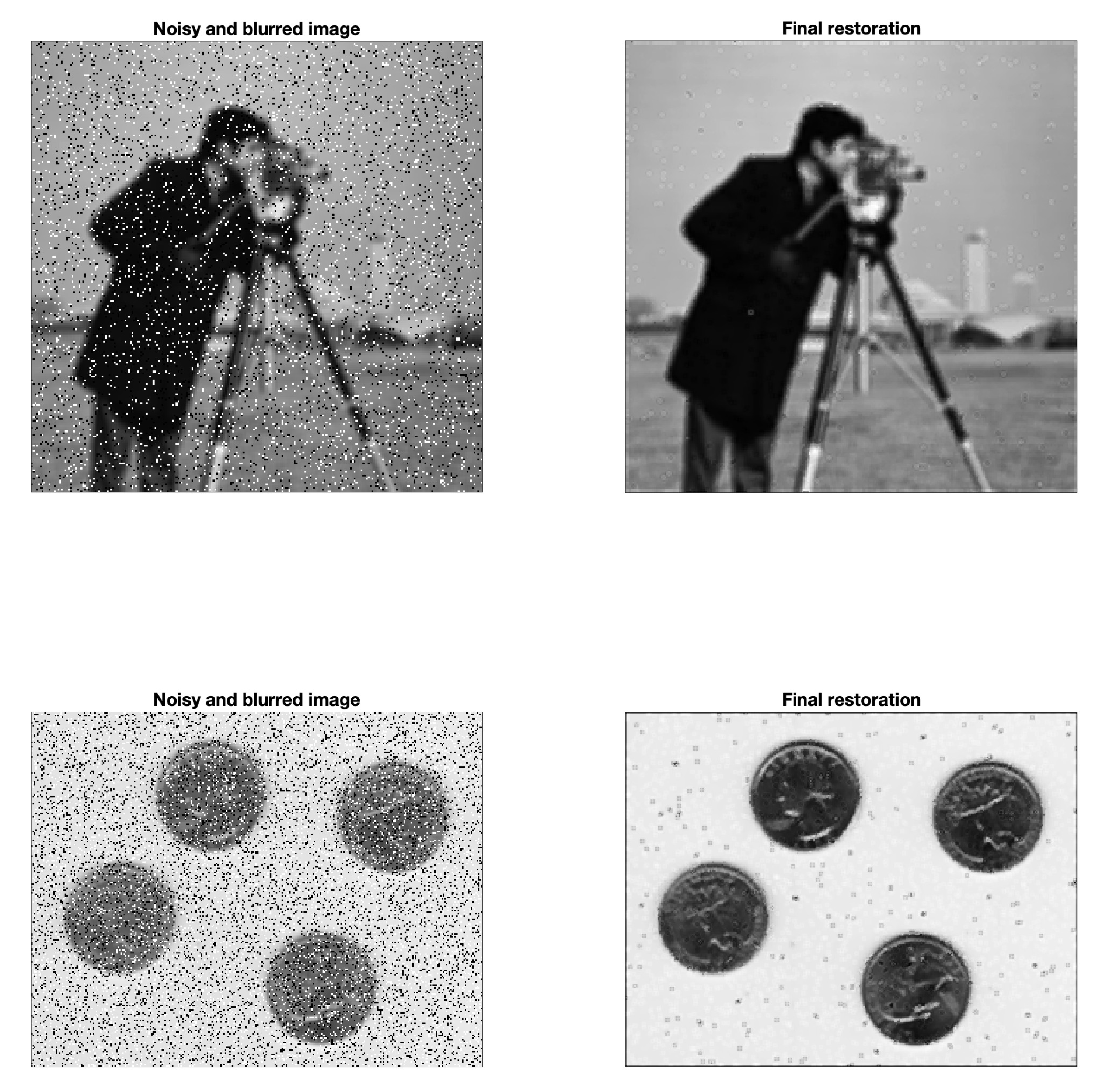
In the following tests, the images are first blurred and then salt&pepper noise is added. Blurring is medium sharp and consists of replacing each pixel with the arithmetic mean of the original neighboring pixel values belonging to a square of size

2 β + 1

β \geq 1

, centered at each point. Moreover, let d denote the noise density, that is the contamination percentage for the salt&pepper noise added to a given image. To be specific a d noise density affects approximately

d %

of the total pixels of the image.

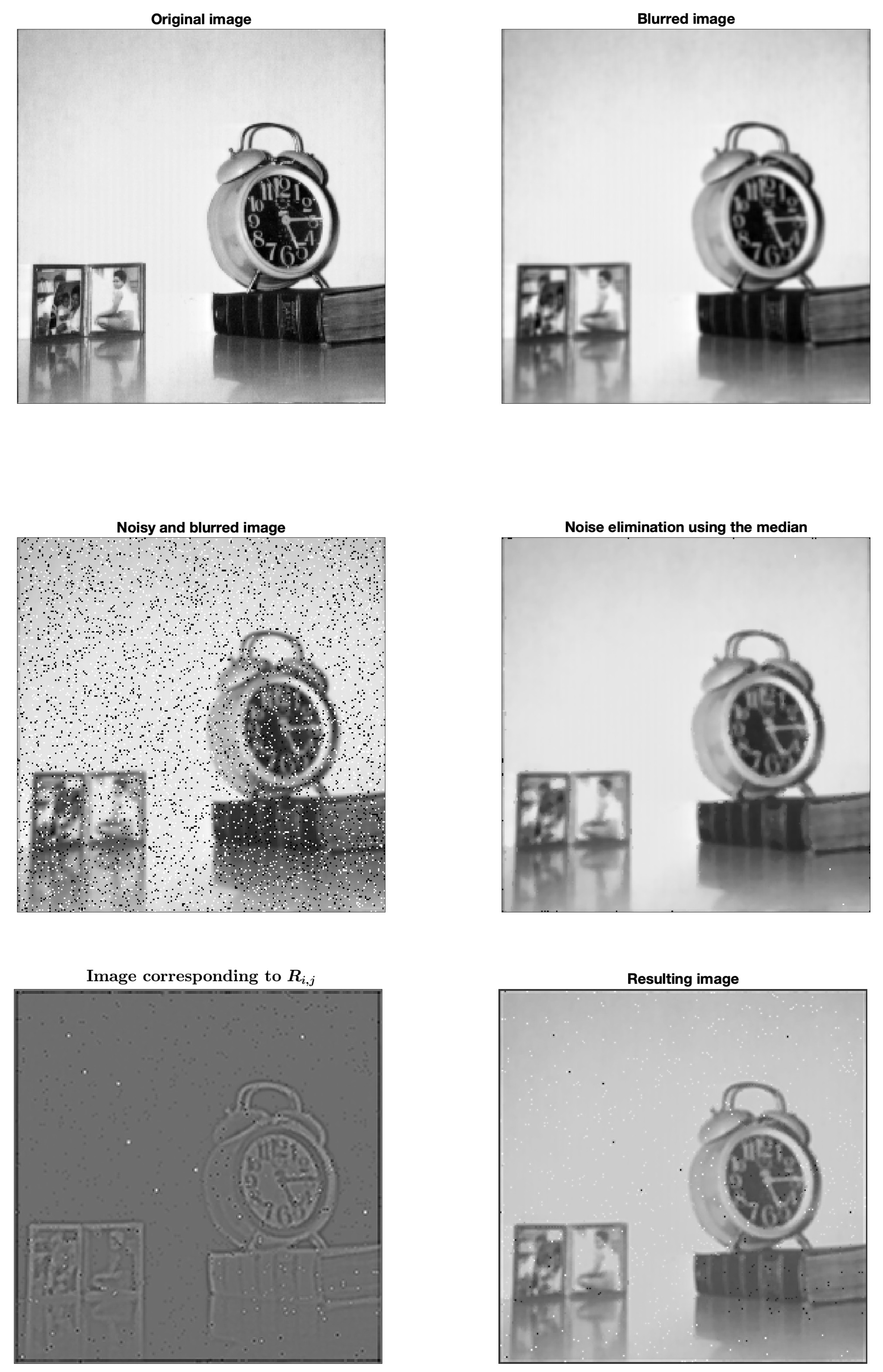
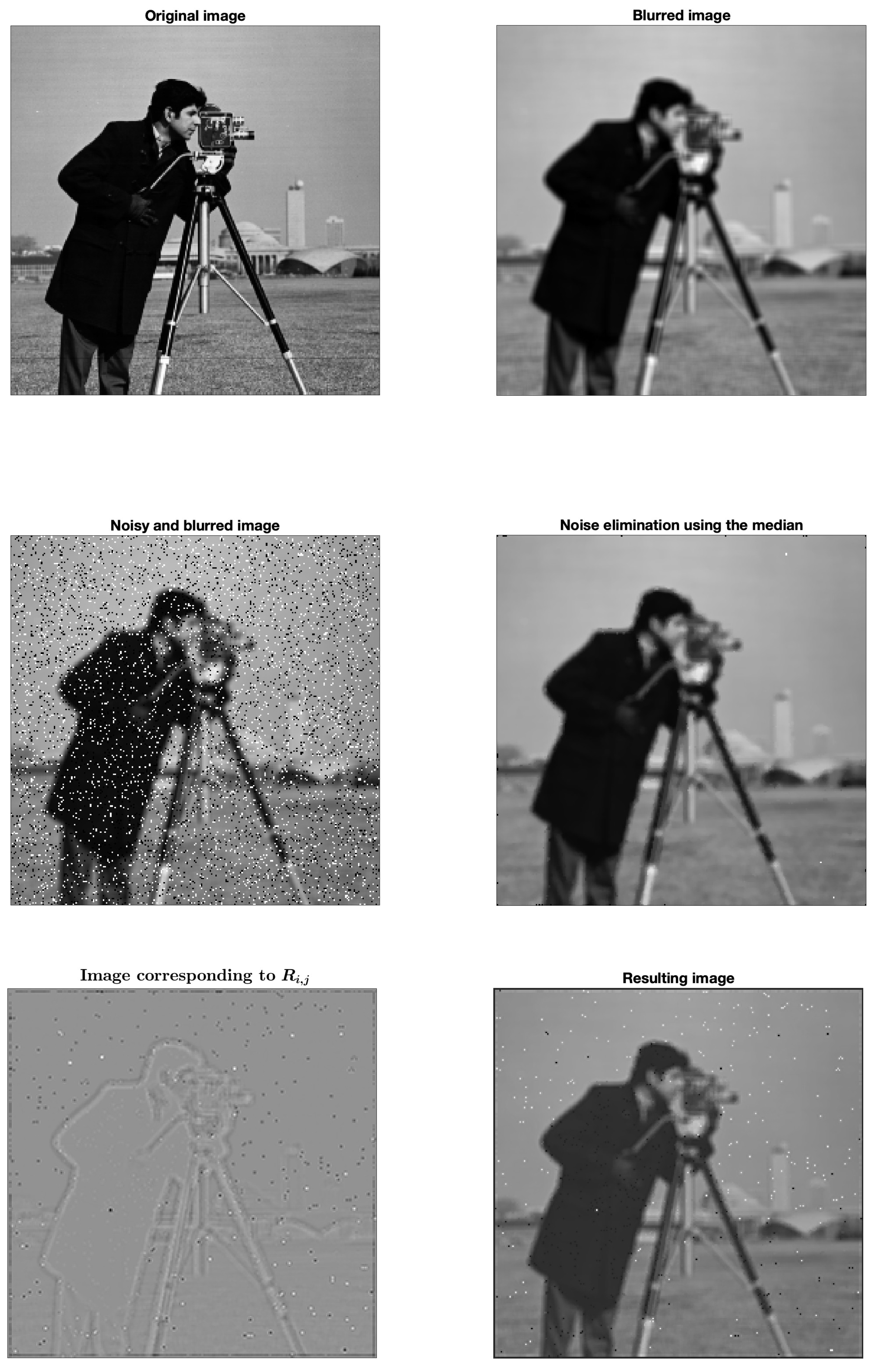
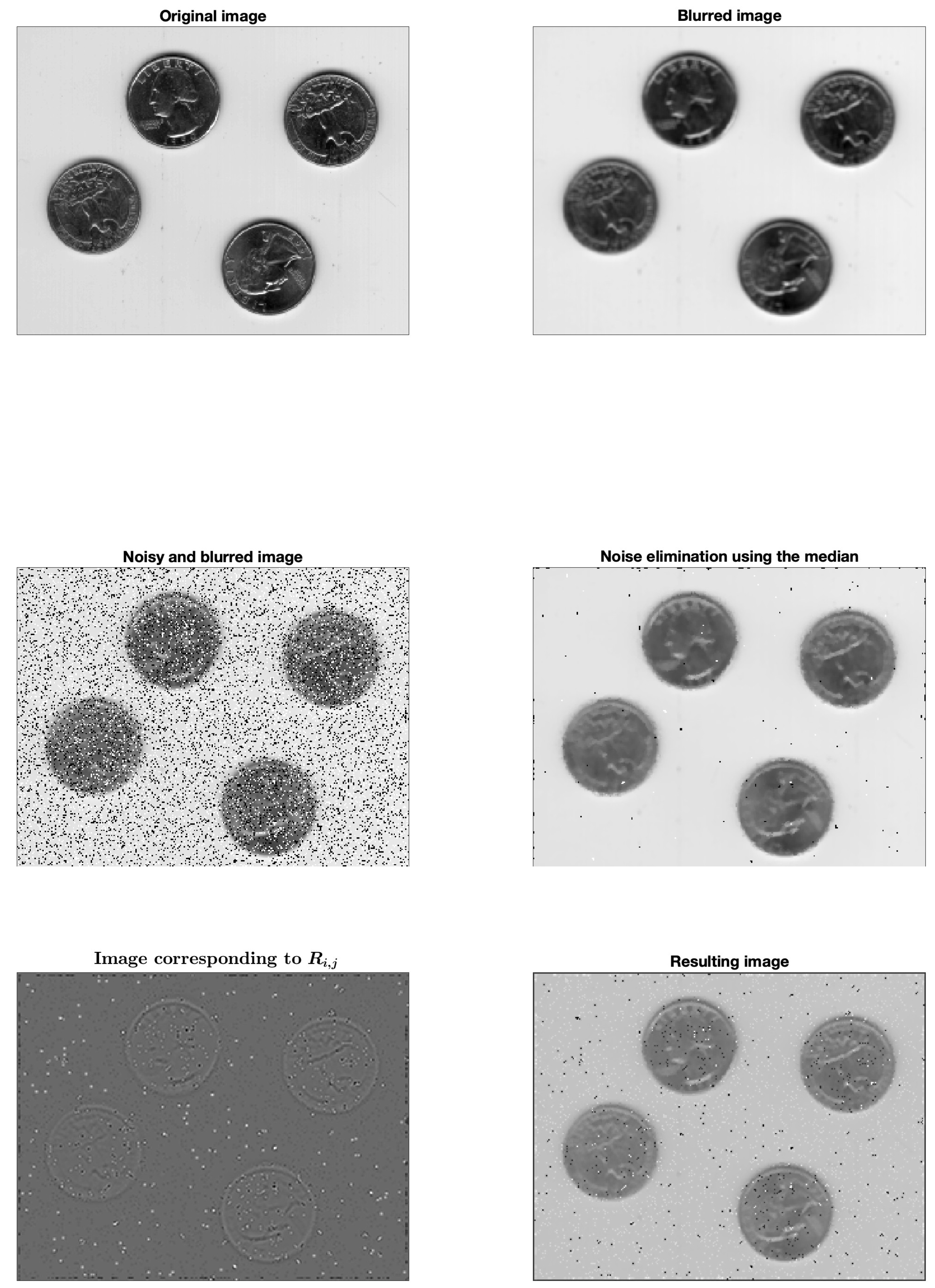
In Figure 3, Figure 4 and Figure 5, the first picture on the top left shows the original image while the top right shows the artificially blurred image. Salt&pepper noise is successively added with different percentage. This brings us to the images in the middle left, where different values of

β

and d were used for each picture. In the middle right we can see this last image treated by applying the median to all points without distinction. That is, each output pixel contains the median value computed from the values belonging to the

3 \times 3

square centered at the corresponding pixel of the input image. The amount of salt&pepper is drastically reduced, but this does not eliminate the blurring which is instead accentuated. Therefore, we will not follow this approach. We apply instead the procedure explained in the previous section for the one-dimensional case. In all the examples that follow we used a grid size

h = 1

. Given the original image defined by the values

u_{i, j}

at the points

(x_{i}, y_{j})

, we compute

R_{i, j}

by applying the nonlinear operator in (9) and the successive interpolation formula (11). The operation amplifies the grains of salt&pepper which can subsequently be filtered by substituting them with the median related to the surrounding

3 \times 3

square. We take, for example, the threshold (see (14) in the 1D case):

τ = \frac{1}{4} (| R_{i - 1, j} | + | R_{i + 1, j} | + | R_{i, j - 1} | + | R_{i, j + 1} |) .

(15)

As specified in Section 3, the correction is only applied at some points, so to produce a reduced increase of blurring. In this way, we get a new cleaner image (not shown) to which we apply the nonlinear operator again to remove the blurring [24,25]. In the lower left pictures we report the new

R_{i, j}

. The edges appear sharpened. The result after one step of the algorithm (12) is finally shown in the lower right corner. In these experiments we choose

γ = - 0.5

. This means that equation (1) is approached with a single explicit backward step. So we are going back in time, and this, thanks to the typology of the operator, allows us to emphasize the contours

The following Algorithm 2 provides a summary of the proposed procedure.

Algorithm 2

Consider the given image determined by the values $u_{i, j}$ at the points $(x_{i}, y_{j})$ ;
Build the discretization (9) of the nonlinear space operator in (1) at the staggered grid points;
By polynomial interpolation, evaluate the quantities $R_{i, j}$ in (11) passing from the staggered to the standard grid;
Remove salt&pepper noise by applying the median filter only where $| R_{i, j} | \geq τ$ , with $τ$ defined in (15);
Apply Algorithm 1 to focus the so obtained image.

The output image of Algorithm 2 is not quite sharp yet, so we will perform one last step by adjusting the contrast. The procedure is explained in the next section. The reason for this last retouching is that the few grains of salt&pepper that have not been filtered predominate the range of variation of the image making the rest appear too uniform.

5. Contrast Adjustment

After the various corrections implemented in the previous section, the final result is quite good but still not optimal. In fact, the image appears greyish. We can improve it by varying the contrast a bit. To this end we make a further iteration by applying the following sigmoid function:

σ (x) = \frac{1}{1 + e^{- b (x - a)}},

(16)

where a is the inflection point and b is the slope parameter. Here

x \in [0, 1]

represents the generic value of the image in the grey scale and

σ \in [0, 1]

the modified value. Usually, the grey scale ranges from 0 to 255, so it is necessary to perform appropriate data scaling before and after processing.

for which it is necessary before and after to do an appropriate scaling of the data.

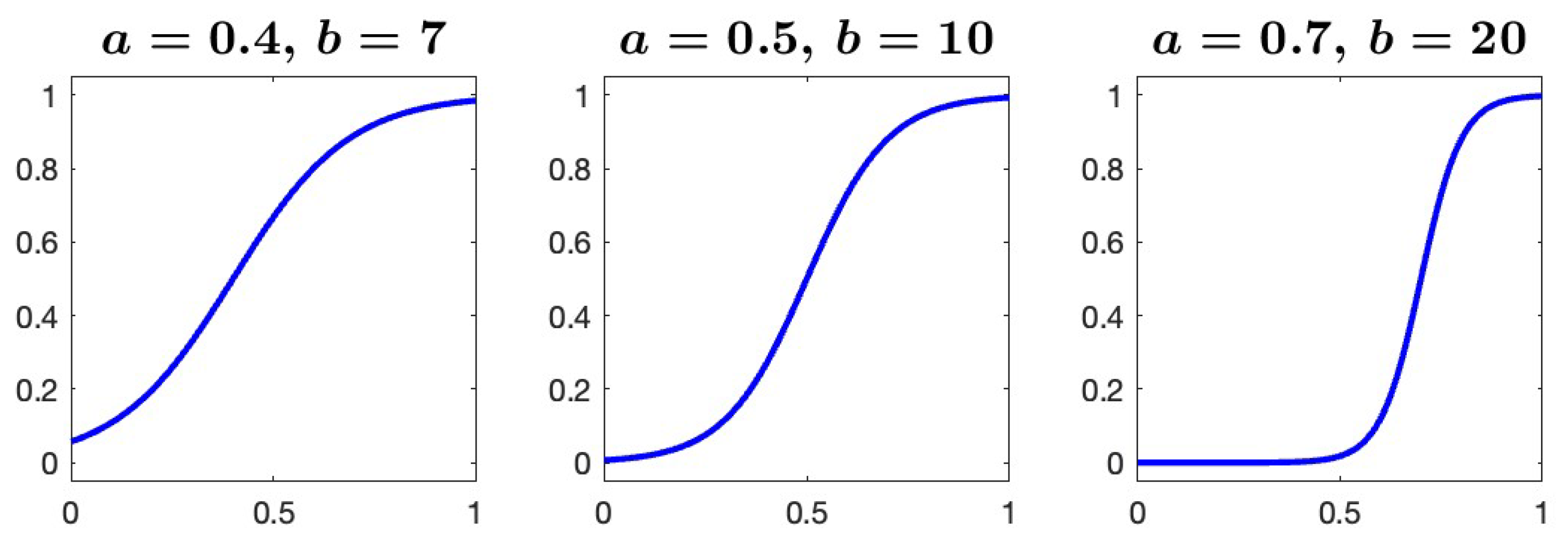
We can see the plots of the function

σ

in Figure 6 for some values of a and b. In particular, in our experiments we used

a = 0.4

and

b = 7

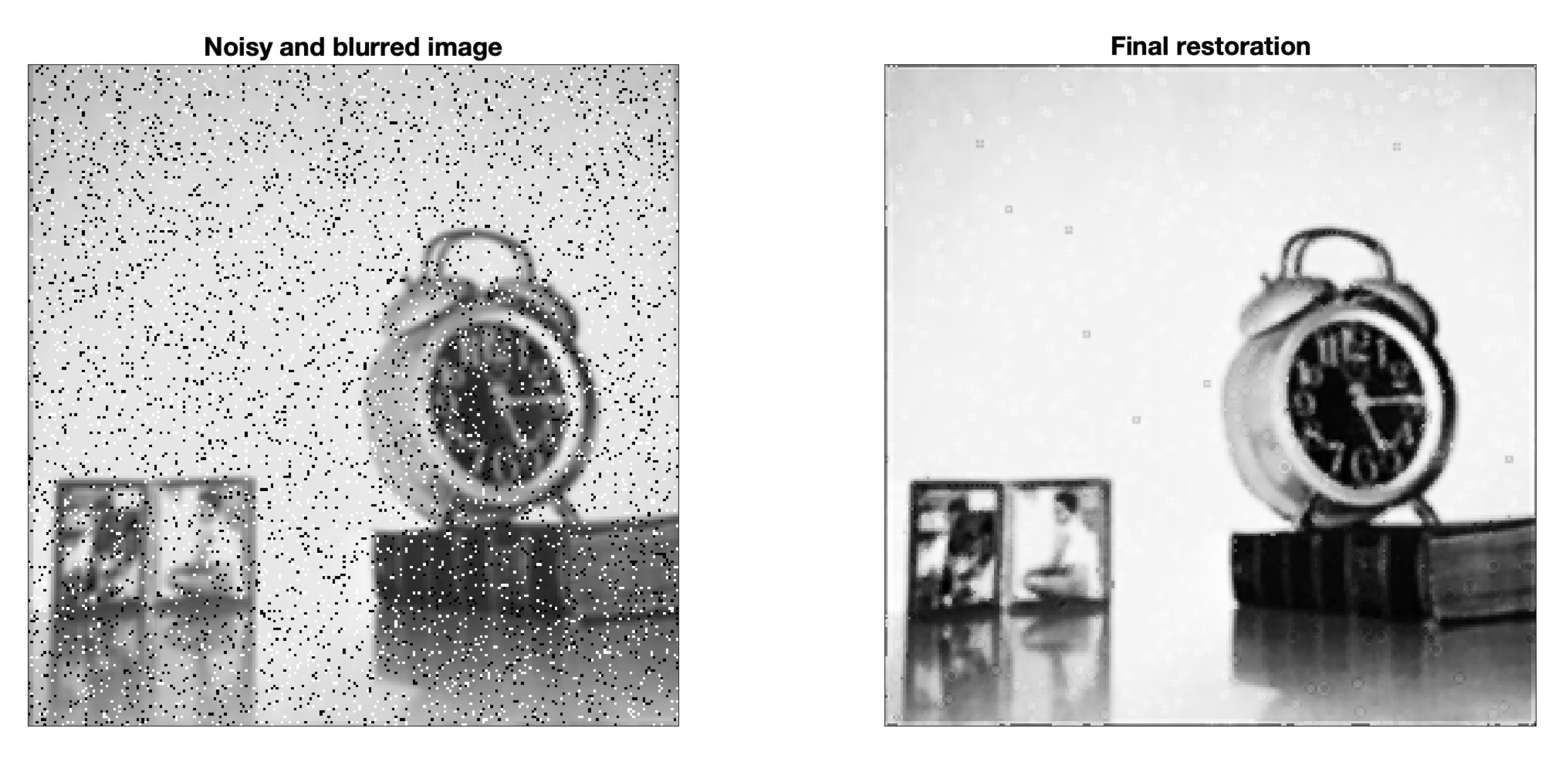
, that is the sigmoid function on the left of Figure 6. Finally, Figure shows the results of our study, where the final image is fairly restored. The whitish parts have become brighter and the dark grey parts have become even darker.

Obviously, depending on the type of images, as well as on the specific applications of interest, different values of the parameters involved in the entire procedure can be selected. The choice of these parameters depends on several factors, such as image resolution, noise density, blur levels, desired image quality, and the specific goals of the application in question. Optimal results can be achieved by customizing parameter values to suit the particular imaging context and application.

Probably other techniques provide similar or even better outcomes, but here it is important to point out that no iterative method has been used. Few steps have actually been made and their cost is proportional to the number of pixels that make up the images. The total cost of the operations is therefore quite low. While this is not essential in 2D applications, it becomes crucial in 3D image analysis.

6. Conclusions

A technique for restoring images affected by various types of noise has been proposed here. The procedure recalls that of nonlinear diffusion, although only a few steps of the algorithm are performed. This involves quite low costs and the final results are comparable to those of other methodologies. We believe that it is possible to further improve performance by acting more carefully on the various parameters available. Potential challenges and directions for future research include the application of the algorithm to three-dimensional images and color RGB images.

Author Contributions

These authors contributed equally to this work.

Funding

This research received no external funding

Acknowledgments

The Authors are affiliated to GNCS-INdAM (Italy).

Conflicts of Interest

The author declares no conflict of interest.

References

Perona, P.; Malik, J. Scale space and edge detection using anisotropic diffusion. IEEE Trans. Pattern Anal. Mach. Intell. 1990, 12(7), 629–639. [CrossRef]
Alvarez, L.; Lions, P.L.; Morel, J.M. Image selective smoothing and edge detection by nonlinear diffusion (ii). SIAM J. Numer. Anal. 1992, 29, 845–866. [CrossRef]
Rudin, L.; Osher, S.; Fatemi, E. Nonlinear total variation based noise removal algorithms. Physica D. 1992, 60, 259–268. [CrossRef]
Coifman R.R.; Donoho, D. Translation-invariant de-noising. In Wavelets and Statistics. Lecture Notes in Statistics (Antoniadis, A., Oppenheim, G.A.; Eds.), Springer, New York, 1995; 125-150.
Donoho, D.; Johnstone, I. Ideal spatial adaptation via wavelet shrinkage. Biometrika. 1994, 81, 425–455. [CrossRef]
Kundur, D.; Hatzinakos, D. Blind image deconvolution. IEEE Signal Process. Mag. 1996, 13(3), 43–64. [CrossRef]
Yaroslavsky, L.; Eden, M. Fundamentals of Digital Optics, Birkhauser, Basel, 1996.
Smith, S.M.; Brady, J.M. Susan - a new approach to low level image processing. Int. J. Comput. Vis. 1997, 23, 45-–78. [CrossRef]
Weicker, J. Anisotropic Diffusion in Image Processing, ECMI Series, Teubner-Verlag, Stuttgart, Germany, 1998.
Sapiro, G. Geometric Partial Differential Equations and Image Analysis, Cambridge Univ. Press, Cambridge, UK, 2001.
Tadmor, E.; Nezzar, S.; Vese, L. A multiscale image representation using hierarchical (bv, l2) decompositions. Multiscale. Model. Simul. 2004, 2, 553–572. [CrossRef]
Buades, A.; Coll, B.; Morel, J.M. A review of image denoising algorithms, with a new one. Multiscale Modeling Simul. 2005, 4(2), 490–53.
Li, S.Z. Markov Random Field Modeling in Image Analysis, 3rd ed.; Springer-Verlag, New York, 2009.
Grasmair, M.; Lenzen, F. Anisotropic total variation filtering. Appl Math. Optim. 2010, 62, 323-339. [CrossRef]
Solomon, C.; Breckon, T. Fundamentals of Digital Image Processing: A Practical Approach With Examples in Matlab, John Wiley & Sons, 2010.
Chaudhuri, S.; Velmurugan, R.; Rameshan, R.M. Blind Image Deconvolution - Methods and Convergence, Springer, 2014.
McCann, M.; Jin, K; Unser, M. Convolutional neural networks for inverse problems in imaging: a review. IEEE Signal Process. Mag. 2017, 34, 85–95. [CrossRef]
Gonzalez, R.C.; Woods R.E. Digital Image Processing, 4th ed.; Pearson, New York, 2018.
Ilesanmi, A.E.; Ilesanmi, T.O. Methods for image denoising using convolutional neural network: a review. Intell. Syst. 2021, 7, 2179–2198. [CrossRef]
Pragliola, M.; Calatroni, L.; Lanza, A.; Sgallari, F. On and beyond total variation in imaging: the role of space variance. arxiv: 2104.03650, 2021.
Kaihao, Z.; Wenqi, R.; Wenhan, L.; Wei-Sheng, L.; Björn, S.; Ming-Hsuan, Y.; Hongdong, Li. Deep image deblurring: a survey. Int. J. Comput. Vis. 2022, 130, 2103–2130. [CrossRef]
Mumford, D.; Shah, J. Optimal approximation by piecewise smooth functions and associated variational problems. Commun. Pure Appl. Math. 1989, 42, 577–685.
Tukey, J.W. Exploratory Data Analysis, Addison-Wesley, Boston, MA, 1997.
Fatone, L.; Funaro, D. High-order discretization of backward anisotropic diffusion and application to image processing. Ann. Università di Ferrara. 2022, 68(2), 295–310. [CrossRef]
Fatone, L.; Funaro, D. An anisotropic diffusion algorithm for image deblurring, in AIP Conference Proceedings of ICNAAM 2022, 2022.

Figure 3. The original image is first blurred (

β = 1

) and then littered with salt&pepper noise (

d = 0.1