Submitted:
10 June 2023
Posted:
12 June 2023
You are already at the latest version
Abstract
Keywords:
1. Introduction
2. Materials and Methods
2.1. Database Generation
2.2. Regression Models
2.3. Database Split and Model Accuracy Measurement
3. Results and Discussion
3.1. Database Exploratory Analysis
3.2. A First Glance in the Predictive Models’ Application
3.3. Deep Diving into Each Predictive Model Group
3.4. Final Models Outcome and Alloy Design Application
4. Conclusions
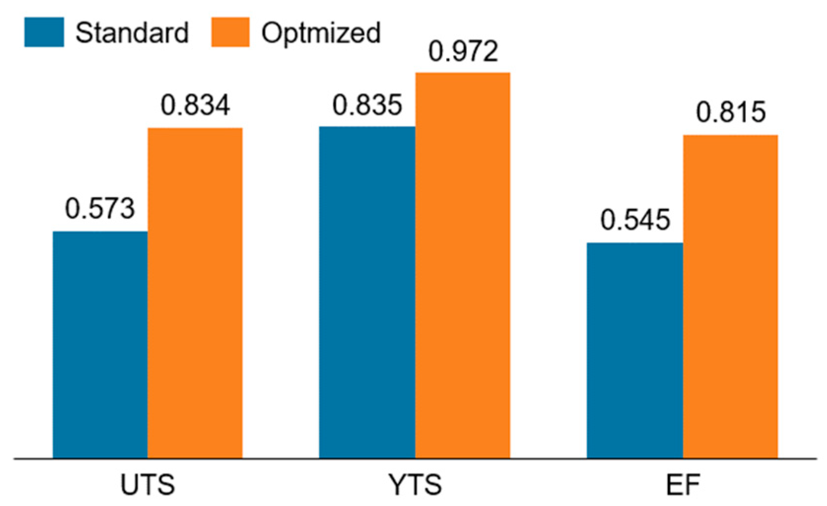
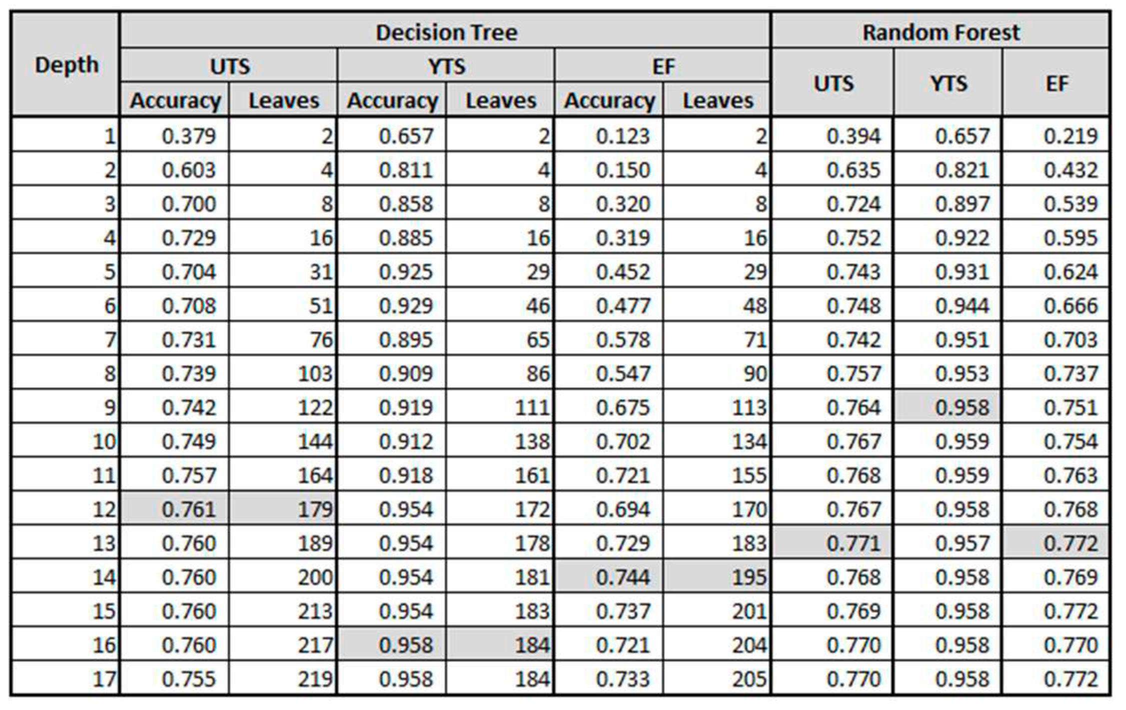
- Although all MLP-optimized models became the best performance found for each variable, the highest increases were related to the YTS and EF. While the first case might be highlighted because of the high accuracy value found, the EF accuracy showed an increase of 0.242, attaining 0.827. This evolution placed the EF predictions in a comparable scenario to the UTS ones, which was first indicated to be a more suitable case.
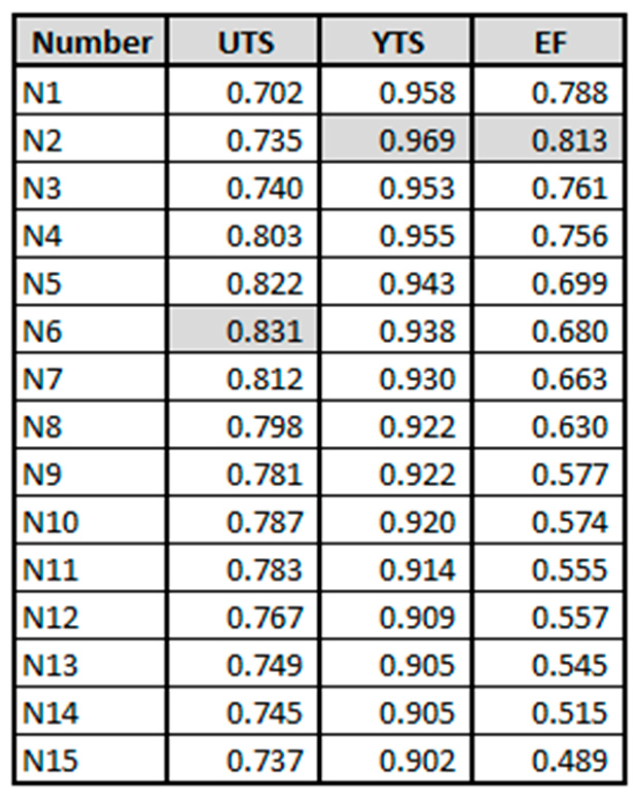
- The KNN-optimized model results were also satisfactory and could be improved from 0.943 to 0.969 for YTS and from 0.699 to 0.813 for EF, with higher performance for smaller number of neighbors.
- It was noted that the alloy design predictions shall not be perfect, but they can be used for sure to indicate a trend. In this sense, the most interesting ones were related to the possible improved UTS based on the Ag and Sb additions, as well as the interesting YTS trends related to Bi-containing alloys modified with Sb.
- Although results could be considered positive, a future study could deep dive into the phase fraction relations of the alloys and investigate a way to enhance the geometrical/spatial” relation behind the attributes. For example, one could use the theoretical models to estimate the non-equilibrium phase fractions forming the alloy microstructures.
Author Contributions
Data Availability Statement
Acknowledgments
Conflicts of Interest
References
- 1. G. E. Moore, Progress In Digital Integrated Electronics. IEDM Tech. Digest.
- Thompson, S.E.; Parthasarathy, E.S. Moore’s law: The future of Si microelectronics. Materials Today 2006, 9, 20–25. [Google Scholar] [CrossRef]
- KRazeeb, M.; Dalton, E.; Cross, G.L.W.; Robinson, A.J. Present and future thermal interface materials for electronic devices. International Materials Reviews 2018, 63, 1–21. [Google Scholar] [CrossRef]
- Sarvar, F.; Whalley, D.; Conway, E. Thermal Interface Materials - A Review of the State of the Art. 1st Electronic Systemintegration Technology Conference, 1292. [Google Scholar]
- Schon, A.F.; Castro, N.A.; Barros, A.D.S.; Spinelli, J.E.; Garcia, A.; Silva, N.C. Multiple linear regression approach to predict tensile properties of Sn-Ag-Cu (SAC) alloys. Materials Letters 2021, 304, 130587. [Google Scholar] [CrossRef]
- Jiang, N.; Zhang, L.; Gao, L.-L.; Song, X.-G. Recent advances on SnBi low-temperature solder for electronic interconnections. J Mater Sci: Mater Electron 2021, 32, 22731–22759. [Google Scholar] [CrossRef]
- Skuriat, R.; Li, J.; Agyakwa, N.; Johnson, C. Degradation of thermal interface materials for high-temperature power electronics applications. Microelectronics Reliability 2013, 53, 1933–1942. [Google Scholar] [CrossRef]
- Garcia, A. Solidificação: Fundamentos e Aplicações, Editora Unicamp, 2007.
- Callister, W.D.; Rethwisch, E.D.G. Materials Science and Engineering: An Introduction, Wiley, 2013.
- Pandas Pydata, pandas DataFrame. Available online: https://pandas.pydata.org/docs/reference/api/pandas.DataFrame.html (accessed on 21 Dcember 2022).
- PyPI, SweetViz. PyPI. Available online: https://pypi.org/project/sweetviz/ (accessed on 21 Dcember 2023).
- Schon, A.F.; Reyes, R.V.; Spinelli, J.E.; Garcia, A.; Silva, B.L. Assessing microstructure and mechanical behavior changes in a Sn-Sb solder alloy induced by cooling rate. J Alloys Compd 2019, 809, 151780. [Google Scholar] [CrossRef]
- Dias, M.; Costa, T.A.; Rocha, O.F.L.; Spinelli, J.; Cheung, N.; Garcia, A. Interconnection of thermal parameters, microstructure and mechanical properties in directionally solidified Sn-Sb lead-free solder alloys. Materials Characterization 2015, 106, 52–61. [Google Scholar] [CrossRef]
- Dias, M.; Costa, T.A.; Silva, B.; Spinelli, J.; Cheung, N.; Garcia, A. A comparative analysis of microstructural features, tensile properties and wettability of hypoperitectic and peritectic Sn-Sb solder alloys. Microelectronics Reliability 2018, 81, 150–158. [Google Scholar] [CrossRef]
- Silva, B.L.; Silva, V.C.E.D.; Garcia, A.; Spinelli, J.E. Effects of solidification thermal parameters on microstructure and mechanical properties of Sn-Bi solder alloys. Journal of Electronic Materials 2017, 46, 1754–1769. [Google Scholar] [CrossRef]
- Osório, W.R.; Peixoto, L.C.; Garcia, L.R.; Mangelinck-Noël, N.; Garcia, A. Microstructure and mechanical properties of Sn–Bi, Sn–Ag and Sn–Zn lead-free solder alloys. Journal of Alloys and Compounds 2013, 572, 97–106. [Google Scholar] [CrossRef]
- Soares, T.; Gouveia, G.L.; Septimio, U.S.; Cruz, C.B.; Silva, B.; Brito, C.; Spinelli, J.; Cheung, N. Sn-0.5Cu(-x)Al solder alloys: microstructure-related aspects and tensile properties responses. Metals 2019, 9, 241–241. [Google Scholar]
- Silva, B.L.; Cheung, N.; Garcia, A.; Spinelli, J.E. Sn–0.7wt%Cu–(xNi) alloys: Microstructure–mechanical properties correlations with solder/substrate interfacial heat transfer coefficient. Journal of Alloys and Compounds 2015, 632, 274–285. [Google Scholar] [CrossRef]
- Hu, X.; Chen, W.; Wu, B.; Hu, X.; Chen, W.; Wu, B. Materials Science and Engineering: A 2012, 556, 816-823.
- Spinelli, J.E.; Garcia, A. Microstructural development and mechanical properties of hypereutectic Sn–Cu solderalloys. Microstructural development and mechanical properties of hypereutectic Sn–Cu solderalloys 2013, 568, 195–201. [Google Scholar] [CrossRef]
- Cruz, C.B.; Kakitani, R.; Silva, B.; Xavier, M.G.C.; Garcia, A.; Cheung, N.; Spinelli, J. Transient Unidirectional Solidification, Microstructure and Intermetallics in Sn-Ni Alloys. Materials Research 2018, 21, 2018. [Google Scholar] [CrossRef]
- Osório, W.R.; Leiva, D.R.; Peixoto, L.C.; Garcia, L.R.; Garcia, A. Mechanical properties of Sn–Ag lead-free solder alloys based on the dendritic array and Ag3Sn morphology. Journal of Alloys and Compounds 2013, 562, 194–204. [Google Scholar] [CrossRef]
- Garcia, L.R.; Osório, W.R.; Peixoto, L.C.; Garcia, A. Mechanical properties of Sn–Zn lead-free solder alloys based on the microstructure array. Mechanical 2010, 61, 212–220. [Google Scholar] [CrossRef]
- Ramos, L.; Reyes, R.V.; Gomes, L.F.; Garcia, A.; Spinelli, J.; Silva, B. The role of eutectic colonies in the tensile properties of a Sn-Zn eutectic solder alloy. Materials Science and Engineering A 2020, 776, 138959. [Google Scholar] [CrossRef]
- Dias, M.; Costa, T.A.; Soares, T.; Silva, B.L.; Cheung, N.; Spinelli, J.E.; Garcia, A. Tailoring Morphology and Size of Microstructure and Tensile Properties of Sn-5.5 wt.%Sb-1 wt.%(Cu,Ag) Solder Alloys. Journal of Electronic Materials 2018, 47, 1647–1657. [Google Scholar] [CrossRef]
- Silva, B.; Xavier, M.G.C.; Garcia, A.; Spinelli, J. Cu and Ag additions affecting the solidification microstructure and tensile properties of Sn-Bi lead-free solder alloys. Materials Science and Engineering A 2017, 705, 325–334. [Google Scholar] [CrossRef]
- Hu, X.; Li, K.; Min, Z. Microstructure evolution and mechanical properties of Sn0.7Cu0.7Bi lead-free solders produced by directional solidification. Journal of Alloys and Compounds 2013, 566, 239–245. [Google Scholar] [CrossRef]
- Spinelli, J.E.; Silva, B.L.; Garcia, A. Assessment of Tertiary Dendritic Growth and Its Effects on Mechanical Properties of Directionally Solidified Sn-0.7Cu-xAg Solder Alloys. J. Electron. Mater 2014, 43, 1347–1361. [Google Scholar] [CrossRef]
- Silva, B.L.; Spinelli, J.E. Correlations of microstructure and mechanical properties of the ternary Sn-9wt%Zn-2wt%Cu solder alloy. Materials Research 2018, 21, e20170877. [Google Scholar] [CrossRef]
- James, G.; Witten, D.; Hastie, T.; Tibshirani, R. An Introduction to Statistical Learning with Applications in R, New York: Springer, 2013.
- Morettin, A.; Singer, J.M. Estatística e Ciência de Dados - Versão Preliminar, São Paulo, 2021.
- Scikit Learn, sklearn.linear_model.LinearRegression. Scikit Leanr. Available online: https://scikit-learn.org/stable/modules/generated/sklearn.linear_model.LinearRegression.html# (accessed on 21 May 2023).
- Educative, Inc, Educative.io. Educative, Inc. Available online: https://www.educative.io/answers/overfitting-and-underfitting (accessed on 1 October 2022).
- Scikit Learn, sklearn.linear_model.Ridge. Scikit Learn. Available online: https://scikit-learn.org/stable/modules/generated/sklearn.linear_model.Ridge.html (accessed on 21 May 2023).
- Scikit Learn, sklearn.linear_model.Lasso. Scikit Learn. Available online: https://scikit-learn.org/stable/modules/generated/sklearn.linear_model.Lasso.html (accessed on 21 May 2023).
- Scikit Learn, sklearn.linear_model.ElasticNet. Scikit Learn. Available online: https://scikit-learn.org/stable/modules/generated/sklearn.linear_model.ElasticNet.html (accessed on 21 May 2023).
- Scikit Learn, sklearn.neighbors.KNeighborsRegressor. Scikit Learn. Available online: https://scikit-learn.org/stable/modules/generated/sklearn.neighbors.KNeighborsRegressor.html (accessed on 1 October 2022).
- Scikit Learn, sklearn.tree.DecisionTreeRegressor. Available online: https://scikit-learn.org/stable/modules/generated/sklearn.tree.DecisionTreeRegressor.html#sklearn.tree.DecisionTreeRegressor (accessed on 13 January 2023).
- Scikit Learn, sklearn.ensemble.RandomForestRegressor. Available online: https://sklearn.ensemble.RandomForestRegressor (accessed on 13 January 2023).
- Bakshi, C.; Random Forest Regression. Levelup.gitconnected. Available online: https://levelup.gitconnected.com/random-forest-regression-209c0f354c84 (accessed on 1 October 2022).
- Scikit Learn, sklearn.svm.SVR. Available online: https://scikit-learn.org/stable/modules/generated/sklearn.svm.SVR.html (accessed on 13 January 2023).
- Scikit Learn, sklearn.neural_network.MLPRegressor. Available online: https://scikit-learn.org/stable/modules/generated/sklearn.neural_network.MLPRegressor.html (accessed on 13 January 2023).
- Scikit Learn, sklearn.model_selection.train_test_split. Scikit Learn. Available online: https://scikit-learn.org/stable/modules/generated/sklearn.model_selection.train_test_split.html (accessed on 13 January 2023).
- Scikit Learn, sklearn.preprocessing.MinMaxScaler. Scikit Learn. Available online: https://scikit-learn.org/stable/modules/generated/sklearn.preprocessing.MinMaxScaler.html (accessed on 13 January 2023).
- Scikit Learn, 3.3. Metrics and scoring: quantifying the quality of predictions. Scikit Learn. Available online: https://scikit-learn.org/stable/modules/model_evaluation.html (accessed on 13 January 2023).
- Python Software Foundation, Python Org. Available online: https://www.python.org/ (accessed on 13 January 2023).
- Clipartmax, Clipartmax. Available online: https://www.clipartmax.com/middle/m2H7i8d3b1m2N4i8_blue-piece-missing-missing-puzzle-piece-clip-art/ (accessed on 13 January 2023).
- Campbell, J. Complete Casting Handbook (Second Edition), Butterworth-Heinemann, 2015, Page 639, ISBN 9780444635099.
- Dieter, G.E. Mechanical Metallurgy, SI Metrics Edition, 1989.
- Scikit Learn. Available online: https://scikit-learn.org/stable/ (accessed on 13 January 2023).







Disclaimer/Publisher’s Note: The statements, opinions and data contained in all publications are solely those of the individual author(s) and contributor(s) and not of MDPI and/or the editor(s). MDPI and/or the editor(s) disclaim responsibility for any injury to people or property resulting from any ideas, methods, instructions or products referred to in the content. |
© 2023 by the authors. Licensee MDPI, Basel, Switzerland. This article is an open access article distributed under the terms and conditions of the Creative Commons Attribution (CC BY) license (http://creativecommons.org/licenses/by/4.0/).


