1. Introduction
Artificial intelligence has helped the fields of computer vision and image literacy flourish. It has also sparked technological advancements in unmanned systems. When compared to other types of conventional marine equipment, unmanned surface vehicles (USVs) are distinguished by their low maintenance costs, low energy consumption, and lengthy periods of continuous operation [
1,
2,
3]. Additionally, USVs can take the place of people to perform difficult and hazardous tasks. As a result, research into USV technology is a reaction to the need for human ocean exploration. The capacity to recognize targets and comprehend the surroundings is one of the core technologies of USV. One of the fundamental technologies of USV is the ability to perceive the environment and identify targets. The USV ought to have a thorough understanding of its surroundings thanks to artificial intelligence technology. For instance, to identify the sort of target at present, the USV sensing technology primarily employs the photoelectric pod to collect optical image data and the LiDAR system to collect point cloud data. The point cloud data set produced by LiDAR is, however, limited in scope and lacking in detail, and the direct processing of the 3D point cloud necessitates powerful computational hardware [
4]. While the optical image of the water surface has the benefits of being simple to collect, having rich color and texture information, and having established processing techniques [
5], using optoelectronic equipment to obtain the intended appearance attributes is a crucial part of how USVs perceive their surroundings.
Deep learning-based optical target detection techniques are now widely used. The two-stage method and the one-stage algorithm are the two categories into which deep learning target identification techniques can be widely divided. Two steps are required to complete two-stage detection. The candidate region is created first. The candidate frame is then classified and regressed using algorithms like R-CNN [
6], Fast R-CNN [
7], and Faster R-CNN [
8]. Single-stage detection, like SSD [
9] and YOLO [
10,
11,
12,
13], uses a convolutional neural network to extract the target's feature information before performing sampling and classification regression operations on the corresponding feature maps using anchor frames with various aspect ratios. Although the two-stage method has a high accuracy rate, real-time requirements are challenging to achieve. Single-stage target detection methods, on the other hand, are far faster and better suited to real-time detection needs. Additionally, single-stage detection techniques are actively being improved; two examples include YOLOv7 [
14] and YOLOv8 [
15]. These models combine the benefits of precision and quickness. In this research, optical target detection on the water surface is investigated using a single-stage detection technique. The following are the paper's main contributions:
A multi-scale feature extraction module is designed to enhance the network's ability to extract target features. Meanwhile, this paper uses the Mish and SiLU activation functions to replace the original activation functions and improve the learning ability of the network.
In this paper, coordinate convolution is used in path aggregation networks to improve the fusion of information from multi-scale feature maps in the upsampling step. Finally, dynamic head is used in the prediction process to effectively combine spatial information, multiscale features, and task awareness.
For USVs, a target detection technique with fewer parameters and reduced computing costs was suggested; it outperforms top lightweight algorithms in a variety of complicated scenarios on water and fully satisfies the timeliness requirements. In addition, a number of model improvement comparison experiments are designated to serve as references for the investigation of techniques for water surface target detection.
The essay is set up as follows:
Section 2 provides an analysis of the approaches employed as well as some current pertinent research work.
Section 3 provides a thorough explanation of the suggested techniques. The experimental findings are presented in
Section 4, along with a comparison of the various approaches and a summary.
Section 5 serves as the essay's conclusion.
2. Related Works
Many researchers have made significant contributions to the field of water surface optical object detection. Deep learning-based object detection algorithms have been effectively used in USVs. Zhangqi Yang et al. [
16] proposed a lightweight object detection network based on YOLOv5. This method is the ultimate in speed and relatively resistant to complex water conditions. Tao Liu et al. [
17] suggested a YOLOv4-based sea surface object detection technique. The improved YOLOv4 algorithm fused with RDSC has a smaller model size and better real-time performance. However, analysis experiments have been conducted on data sets with relatively homogeneous scenarios. There have also been many recent studies on how to improve target detection accuracy. Yuchao Wang et al. [
18] proposed an improved YOLOX_s network ship-target detection algorithm. The Spatial Attention Module (SAM) is integrated into YOLOX's backbone network to focus on detecting the target from the spatial dimension and improve the detection accuracy. The same problem is that the experiments are only conducted on a single dataset, which has too many targets with the same background and a single scene, and the accuracy improvement effect is not necessarily applicable to multi-scale targets and complex scenes. Ruixin Ma et al. [
19] proposed a method. They improved the anchor box through the attention mechanism and false detection. But they didn’t concentrate on the demand for real-time detection at the terminal. Zeyuan Shao et al. [
20] proposed an enhanced convolutional neural network named Varifocal Net that improves object detection in harsh maritime environments. This approach improves detection in harsh water environments but is mainly optimized for small targets and is not applicable to multi-scale targets on the water surface, and the use of deformable convolution (DCN) will greatly increase the inference time.
Some of the aforementioned study components are too focused on detecting speed, while others disregard timeliness. Without further integrating various water conditions and the characteristics of targets, others have only been researched in a single scenario. For mobile applications like USV, this research suggests a lightweight detection approach with improved feature fusion. While fully fulfilling the real-time performance, complicated scene detection is accomplished with greater accuracy.
3. Materials and Methods
3.1. YOLOv7-tiny Detection Framework
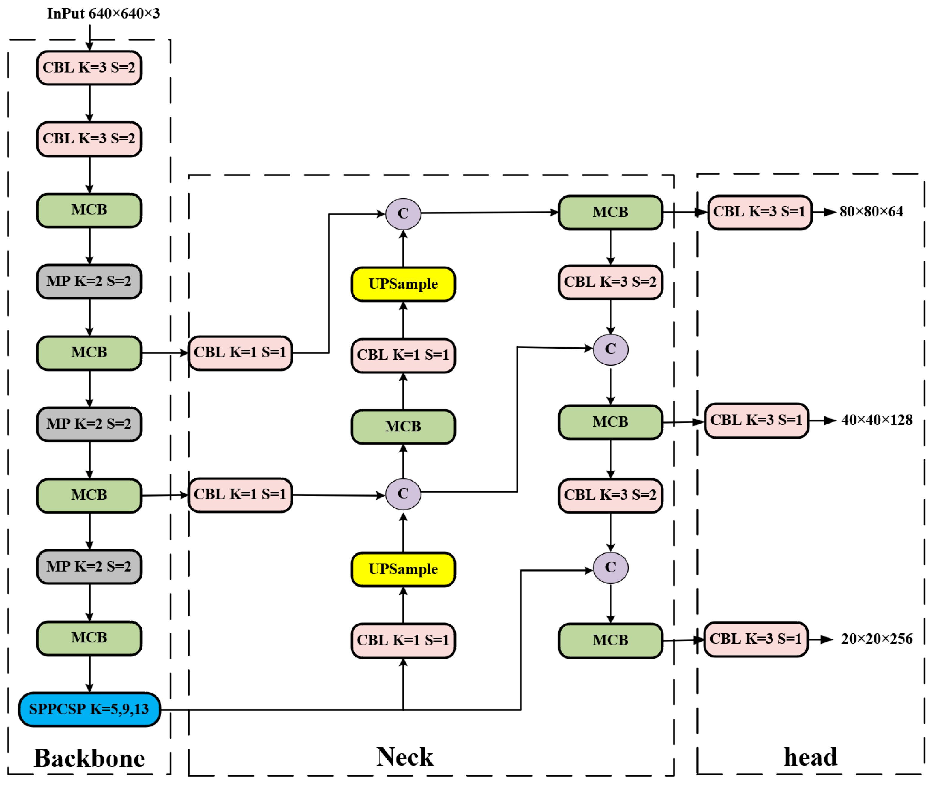
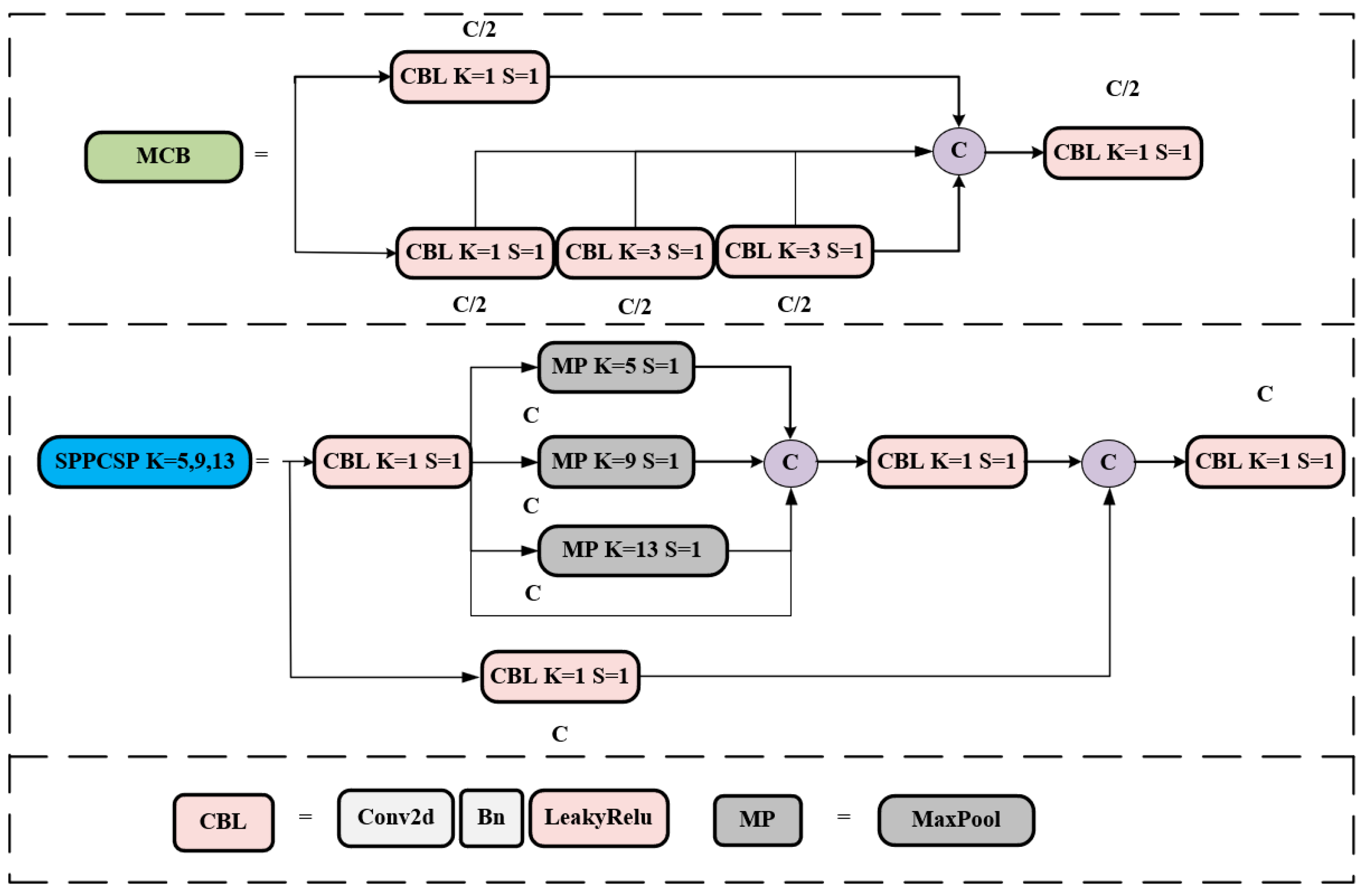
Yolov7 was proposed by the team of Alexey Bochkovskiy, the author of Yolov4, on August 20, 2022. Its performance on the COCO dataset is excellent, and its model accuracy and detection speed are unquestionably first in the interval from 5 to 160 FPS. Yolov7-tiny, on the other hand, is a lighter version of Yolov7, whose network structure is shown in
Figure 1, and the structure of each module is shown in
Figure 2.
3.1.1. Backbone Network
The backbone network of Yolov7-tiny consists of CBL modules, MCB modules, and MP modules, the structure of which is shown in
Figure 1. The CBL module consists of a convolutional layer, a batch normalization layer, and a LeakyReLU layer, which sets the convolutional kernel size to 1 to change the number of channels in the feature map. When the convolutional kernel size is set to 3, if the step size is 1, it is mainly used to extract features; if the step size is 2, it is used to down-sample. The MCB is an efficient network structure. It has two main branches, which enable the network to extract more feature information and have stronger robustness by controlling the shortest and longest gradient paths. One of which is through a CBL module; the other branch’s first goes through a CBL module for changing the number of channels, and then through two CBL modules for the features to be extracted, each passing through a CBL module to output one feature. Finally, the four output features are superimposed and output to the last CBL module. The backbone down-sampling method starts with two convolutions of step size 2, followed by a maximum pooling (MP) module of step size 2, with each down-sampling halving the feature map size.
3.1.2. Head Network
Yolov7-tiny's Head network adds SPPCSP, MCB, and CBL modules on top of the path aggregation network (PaNet) to achieve better multi-scale feature fusion, where the SPPCSP module has two branches, one of which has only one CBL module, while the other branch is more complex. The first goes through a CBL module, followed by performing pooling kernels of 13, 9, and 5 for MP, and then stacking operations, again going through a CBL module. Then performing channel fusion with the other branch and feeding the fused output into the last CBL module to get the output.
3.1.3. Prediction Network:
The I-Detect detecting head is used as the Yolov7-tiny network's output. The CBL module serves to gather features and adjust the number of channels after the MCB module has extracted the feature network at three different sizes. To anticipate targets of various sizes, feature maps with channel counts of 64, 128, and 256 are output in three different sizes.
3.2. The Mish and SiLu Activation Function
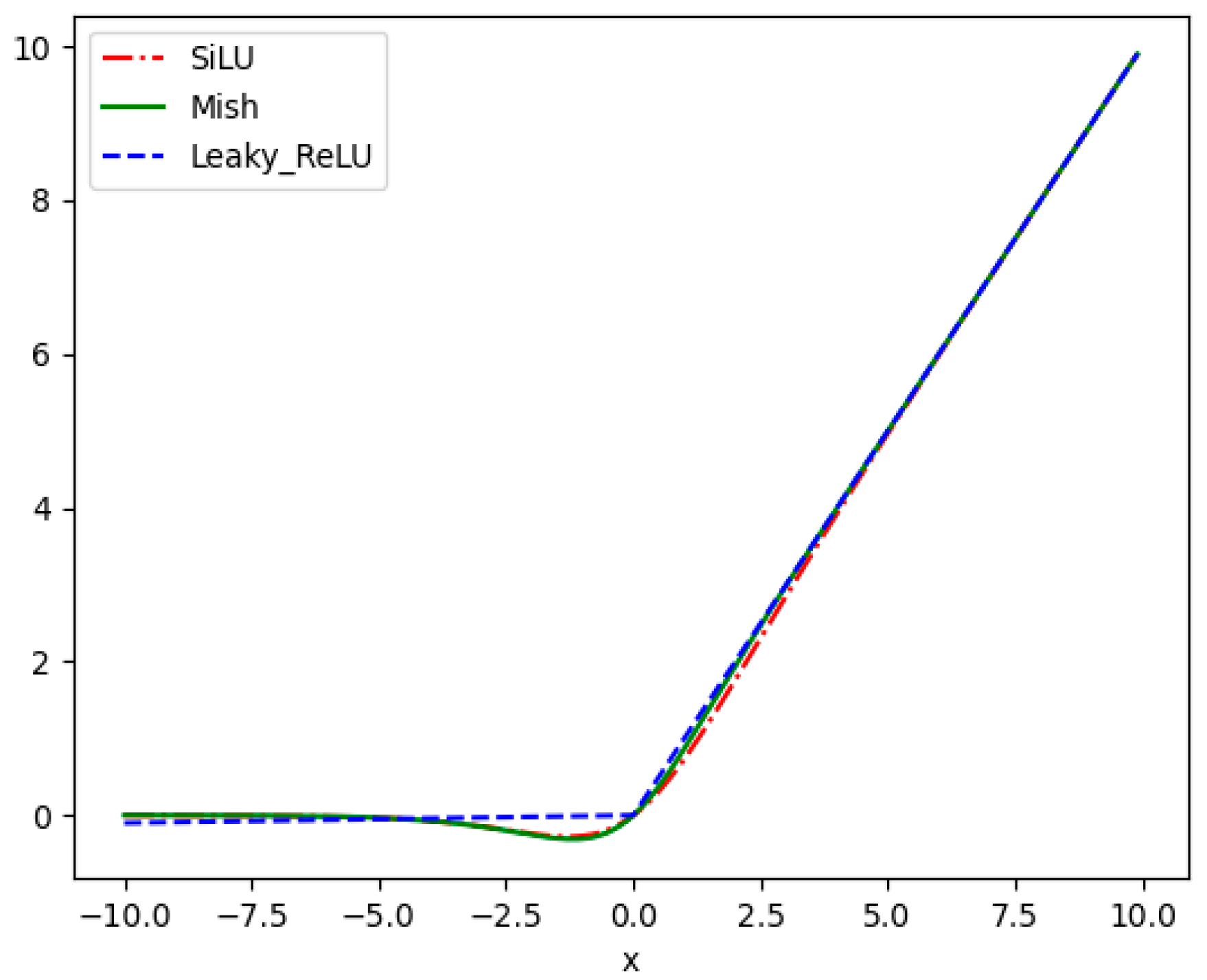
Fewer feature extraction operations are necessary due to the lightweight model's limited number of parameters and calculations. Without raising deployment costs, the model can learn and perform better when the appropriate activation function is used. To circumvent the difficulty of establishing a consistent link between positive and negative input values, LeakyReLU [
21] is substituted with the activation functions Mish and SiLU [
22,
23]. The equations they possess are as follows:
The replacement activation function can achieve the minimum value at zero, which self-stabilizes and buffers the weights. The gradient calculation is made easier by the more derivable activation functions Mish and SiLU. This improves the feature extraction network's performance. In order to prevent the delayed convergence brought on by a zero gradient during network training, the Mish and SiLU activation functions have a lower bound but no upper bound, as seen in
Figure 3, and the gradient is near 1. It is possible to prevent the issue of sluggish convergence brought on by a zero gradient. The length of LeakyReLU is not truncated in the negative interval. However, compared to LeakyReLU activation functions, the Mish and SiLU activation functions are smoother, adding more nonlinear expressions and enhancing the model's capacity for learning.
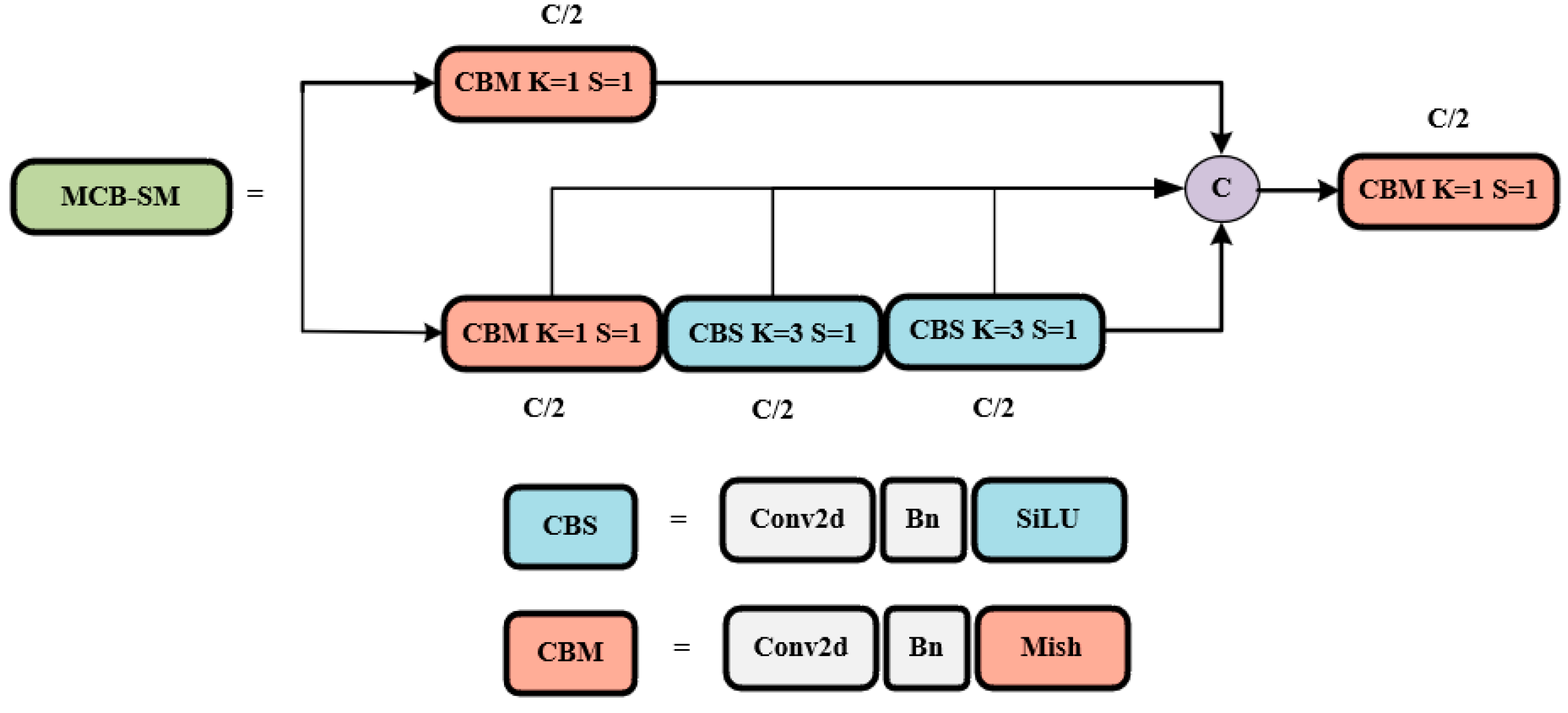
In this study, the MCB-SM module uses these two activation functions, as shown in
Figure 4. Later, they will also be utilized in the neck, head, and modules created for this paper.
3.3. Design of Res2Block
This section introduces the Res2Block, which is more compact and aims to enable a more thorough fusion of multi-scale water surface target properties.
The Multi Concat Block, or MCB for short, is a crucial feature extraction technique for the Yolov7-tiny and is used repeatedly in the backbone and neck to aggregate useful features. However, the multiple-stacked feature extraction's convolution parameters and computing effort are quite significant. Targets on the water surface come in a wide variety of kinds, sizes, and aspect ratios. Understanding the observed object as well as the surrounding environmental context requires knowledge of multiscale feature information. The accuracy of future surface sensing activities like tracking and re-identification will be impacted if the multi-scale features in the water surface environment are not properly retrieved. As a result, the Res2Block module is built and proposed in this study in relation to the Res2Net [
24] network architectural concept.
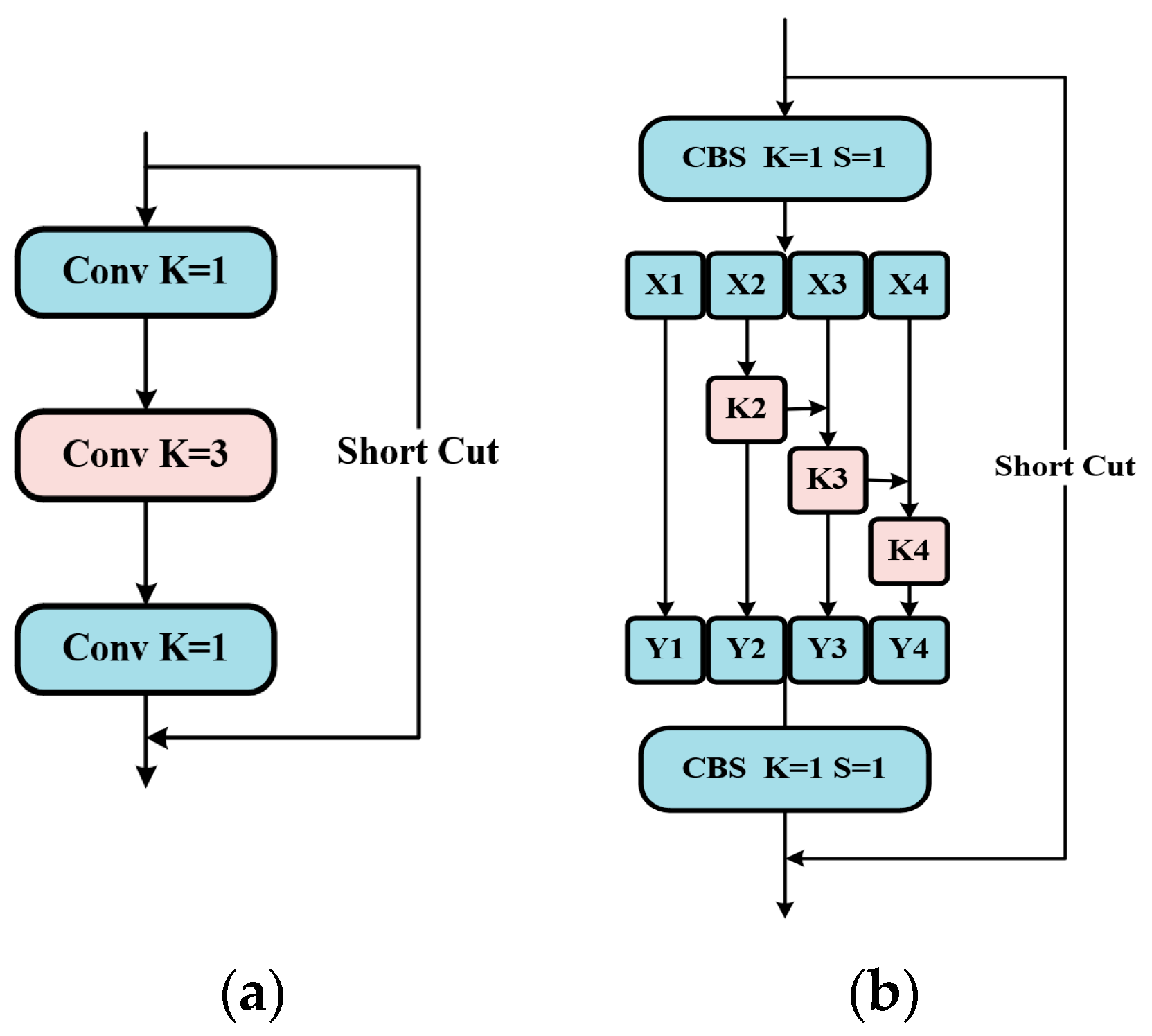
By replacing a set of convolutions with a smaller set of convolutions and linking several filter sets in a hierarchical residual-like manner, the reference paper for Res2Net proposes to build the feature extraction network structure. The Res2Net module, or R2M for short, is the proposed neural network module's moniker since it entails residual-like connections within a single residual block.
Figure 5 shows the difference between the Bottleneck block and the R2M module, which are commonly used in common network junction structures. After a CBS module, R2M divides the feature mapping uniformly into subsets of feature mappings, denoted by
, where
. Each feature subset
has the same spatial size, but with
number of channels. Each
has a corresponding convolution with a 3×3 filter denoted by
, except for
. We denote the output of
by
. The feature subset
is added to the output of
and then fed into
. To reduce the parameters while adding
, the convolution of
is omitted. Thus,
can be written as:
Each may receive feature information from all feature splits . Each time a feature split goes through a convolution operator with a 3×3 filter, the output can have a larger receptive field than . Each time a feature split passes through a convolution operator with a 3×3 filter, the output can have a larger receptive field than .
The Res2Net module processes features in a multi-scale way for splitting, facilitating the extraction of global and local information. The output of the Res2Net module contains various numbers and combinations of receptive field size scales. All splits are interconnected, allowing for more effective processing of features by 1:1 convolutional splits and cascading techniques that can force convolution. The first split's convolution decreases the number of parameters, which is sometimes referred to as feature reuse. Use as a scale dimension control parameter.
Figure 6 illustrates how Res2Block is further designed in this study to more effectively incorporate multi-scale features.
After a convolutional with the SiLU activation function, the number of channels is halved in a split operation. The feature map with the halved number of channels is then stacked with the other two halved branches to form a feature map with 1.5 times the number of channels after a Res2Net module. Finally, the result is output after another convolutional with the SiLU activation function. Compared with the MCB module in the original network, the method in this paper reduces the computationally intensive stacking of the feature extraction convolutions with 3×3 filters and introduces richer multi-scale information. In this paper, the MCB module with 128 and 256 down-sampling channels in the backbone and neck is replaced by the designed Res2Block because the number of channels processed corresponds to a larger number of parameters. It is demonstrated that the proposed Res2Block reduces the number of parameters and computational effort and, at the same time, improves the detection accuracy of water surface targets.
3.4. Neck Combined with CoordConv
USVs performing water surface target detection tasks usually face complex spatial environments such as rain, fog, upwelling, backlight, and background interference. This paper introduces coordinate convolution (CoordConv) [
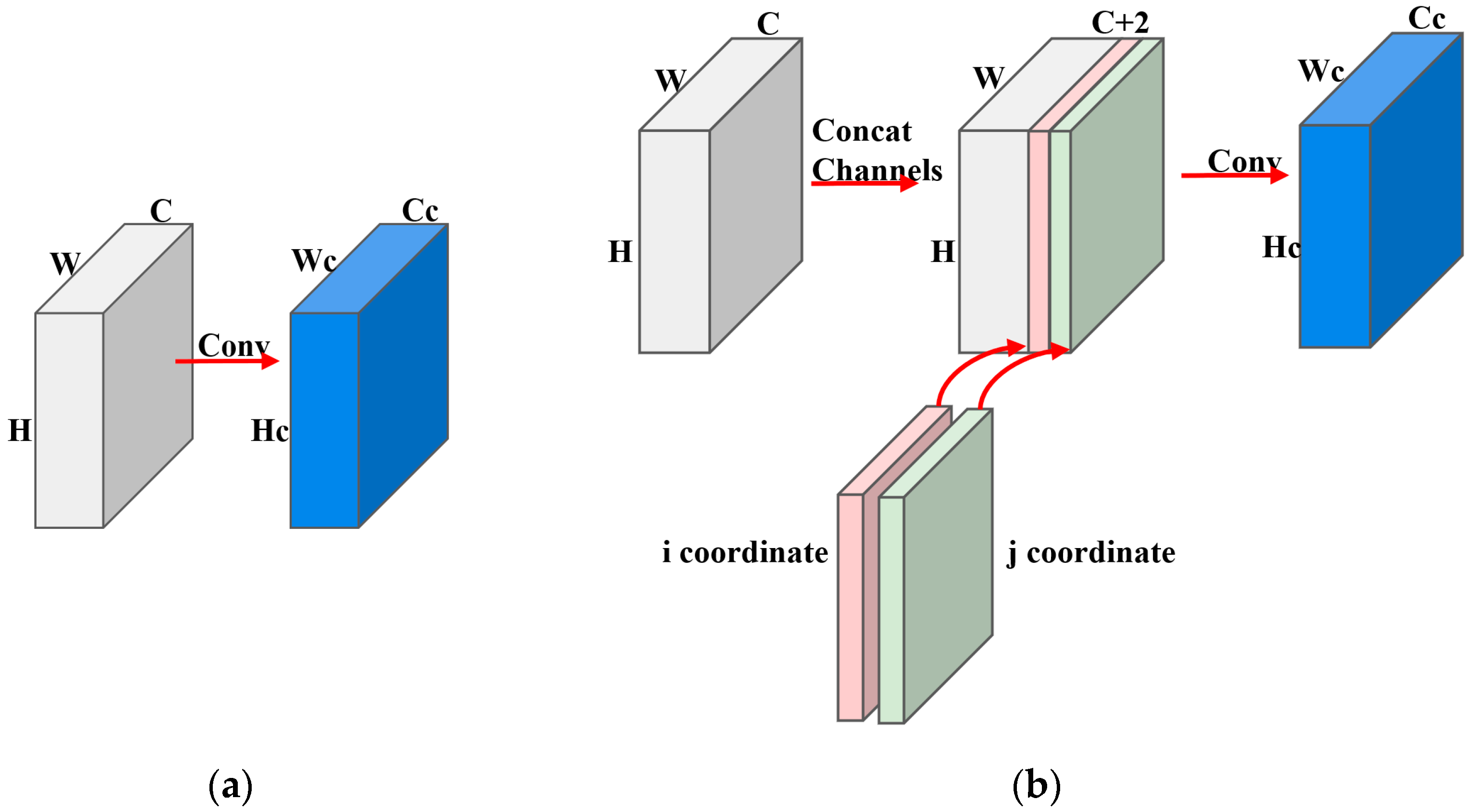
25] to replace normal convolution. Combining CoordConv inside a path aggregation network (PaNet) can effectively reduce the loss of spatial information in the feature fusion process for multi-scale targets. Compared with normal convolution, CoordConv adds a coordinate channel for convolutional access to Cartesian spatial information. Without sacrificing the computational and parametric efficiency of ordinary convolution, CoordConv allows the network to learn to choose between full translational invariance or varying degrees of translational dependence depending on the specific task. Translational invariance means that the network produces the same response (output) regardless of how its inputs are translated in image space. It can capture the spatial information of the target more accurately and reduce information interference such as angle and position transformation in multi-scale targets. The principle is illustrated in
Figure 7:
CoordConv can be implemented based on a simple extension of the standard convolution, adding two channels and filling in the coordinate information. The operation of adding two coordinates
and
is depicted in (b) in
Figure 7. Specifically, the
coordinate channel is an
matrix with 0 in the first row, 1 in the second row, and 2 in the third row. The
coordinate channels are filled with constants in the same way as the columns, and the coordinate values of
and
are finally scaled linearly to keep them within the range of [–1, 1]. And the two coordinates are finally integrated into a third additional channel
coordinate with the following formula:
While enhancing the perception of spatial information, CoordConv allows for a flexible choice of translation invariance based on network learning. The principle is similar to residual connectivity and enhances the generalization capabilities of the model to a certain extent. With a negligible number of bias parameters, a standard convolution with a convolution kernel of and channels ofwill containweights. While after a CoordConv contains weights of .The and coordinate operations are added when is taken as 2, and thecoordinate operation is added when is taken as 3.
Yolov7-tiny uses PaNet on the Neck for multi-scale feature extraction and fusion. In this paper, CoordConv is introduced to Neck and Head, replacing the normal convolution in the up-sampling part of PaNet and all convolutions in the Head part, and introducing the third channel coordinate information. The experimental results show that the improved network effectively combines spatial information with an almost negligible increase in the number of parameters and enhances the fusion of multi-scale target features.
3.5. Head Combined with Dynamic Head
The detection of water surface targets faces challenges of position change, angle switch, and scale change. The Yolov7-tiny detection head does not combine multi-scale information, spatial information, and task information well. This paper combines dy-namic head (DyHead) [
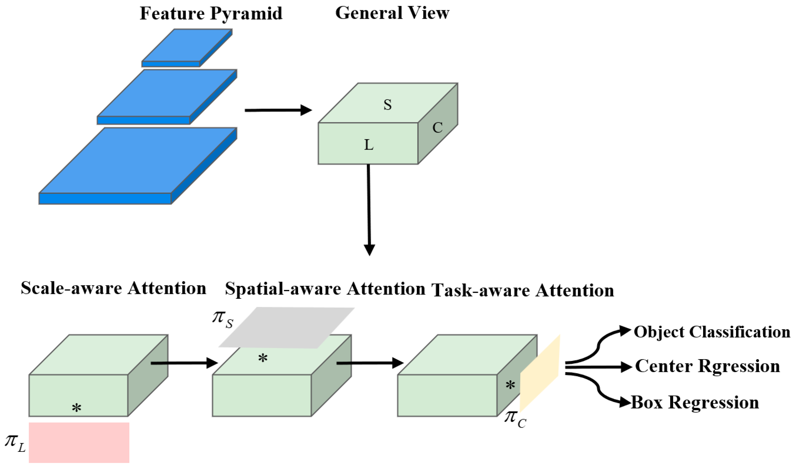
26] to enhance the adaptability of the original model for surface target detection tasks. The principle of DyHead is shown in
Figure 8:
The
different levels of the feature pyramid output are scaled in series as
, where
is the number of pyramid levels.
,
and
are the width, height, and number of channels of the intermediate-level features respectively. Further define
, to obtain the 3D tensor definition
. For the above given tensor, the general equation when combined with attention is:
where
tabulates the attention function, and in practice, this function is encoded through one fully connected layer. However, as the network deepens, it becomes computationally expensive to do the attention function learning directly on a high-dimensional tensor in this way. Therefore, Dy-Head divides the attention function into three parts, as shown in
Figure 8, with each part focusing on only one perspective. This is shown in the following equation:
where
,
and
are the three functions applied to
,
and
, respectively. Scale-aware attention is first fused to fuse semantic information at different scales, as shown in the equation:
where
is a linear function approximated by a 1×1 convolutional layer and
is a hard S-shaped function.
Secondly, considering the high tensor dimensionality in
, the spatially aware attention module is decomposed into two steps: The spatially aware attention module is decomposed into two steps: The process of first using deformable convolutional sparse attention learning and then aggregating images across layers at the same spatial location is shown in the equation:
where
is the number of sparsely sampled locations,
is a location offset by a self-learning spatial offset
to focus on the discriminative region, and
is the self-learning importance scalar at the
location. Both are learned from input features at the median level of
.
Finally, task-aware attention was deployed. It dynamically switches the function's on and off channels to support different tasks: the rationale is shown in the equation:
where
is the feature slice of the
channel,
is a hyperfunction that learns to control boundary of the activation function.
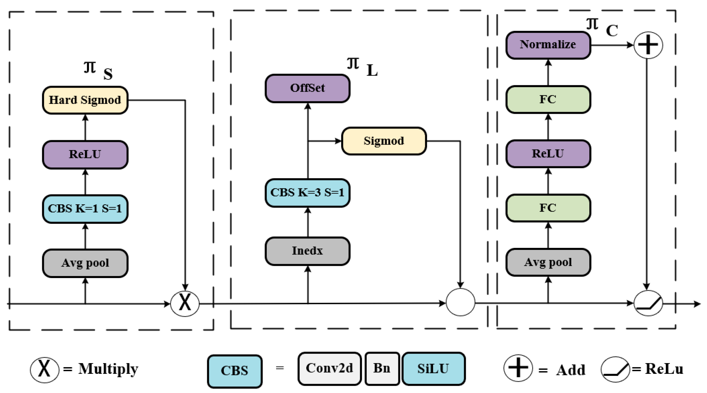
is implemented similarly to dynamic ReLU, which first performs global averaging pooling in the
dimension to reduce the dimensionality, t then employs a normalization layer, two fully linked layers, and a shift-ed S-shaped function to normalize the output to [-1, 1].
Figure 9 illustrates the DyHead network structure used with the Yolov7-tiny.:
In this paper, the original detector head is replaced by the DyHead, and the number of channels in the prediction output is adjusted to 128. This improvement allows the detector head to capture more detailed information about the target and thus predict it more accurately.
3.6. The Proposed YOLOv7-RCD Model
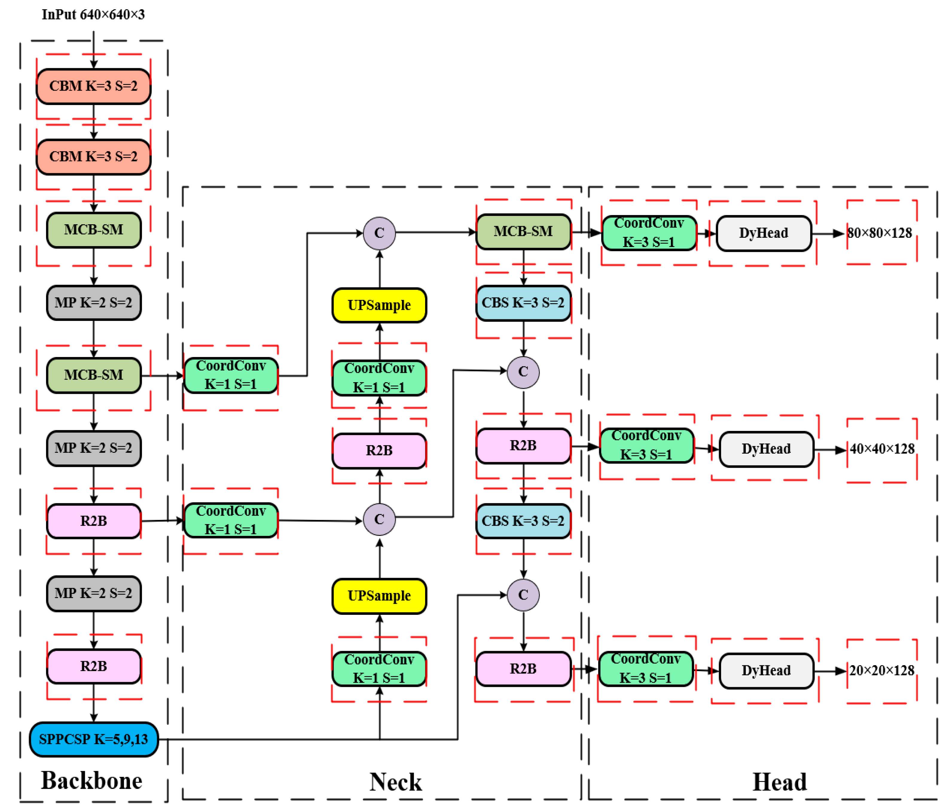
The improved Yolov7-RCD network is shown in
Figure 10:
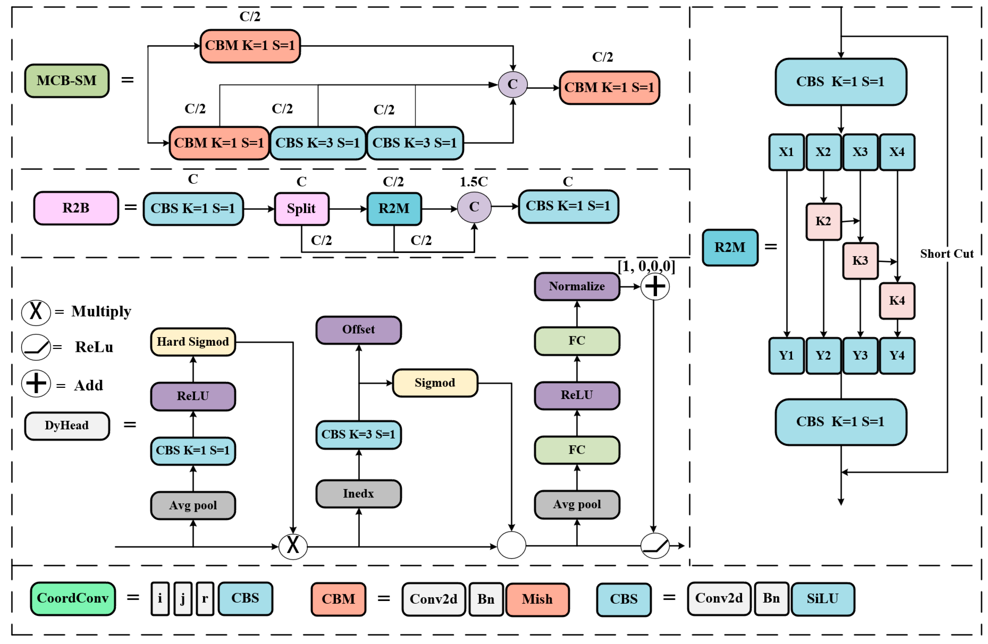
In
Figure 11, the altered components are shown by red boxes. After replacing the network backbone input with Mish and all MCB modules with at least 128 output channels with R2B, the activation function for the down-sampling convolution with two consecutive steps of 2 is used. The number of output channels remained constant from the outset. SiLU is used in place of PaNet's activation functions for the two-step down-sampling convolution. With three additional channels of coordinate information, CoordConv takes the place of regular convolution in the up-sampling and detection headers. In the end, DyHead is included, bringing the total number of output prediction channels to 128.
4. Experiments
To validate the effectiveness and superiority of the proposed YOLOv7-RCD model in a challenging water surface detection environment. The platform and the parameters of the experiment are configured as follows.
4.1. Experimental Environment and Parameter Setting
The platform of this experiment is as following
Table 1:
The experimental parameters are set as shown in the following
Table 2:
4.2. Introduction to USV and Datasets
Validating the performance of data-driven deep network algorithms is generally done on large, publicly available datasets. However, at this stage, there are no large publicly available datasets suitable for water surface target detection. And a single dataset has limited scenarios, and the training results are not sufficient to illustrate the learning capability of the model. In this paper, we extracted part of the images from SeaShip7000 [
27], the Water Surface Object Detection Dataset (WSODD) [
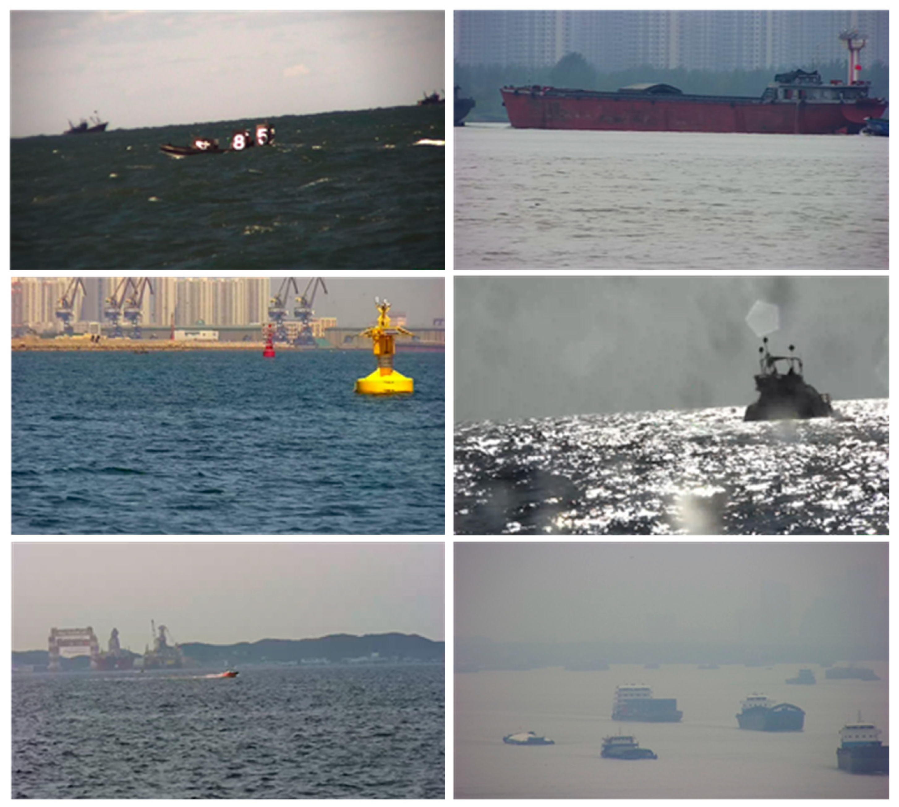
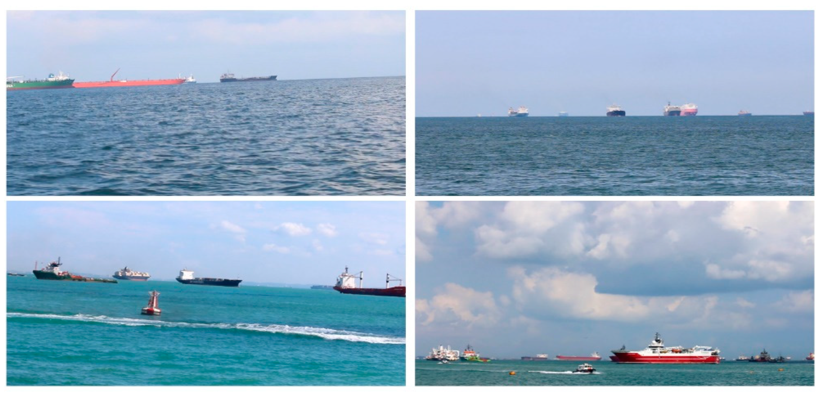
28], and realistic and reliable data from a USV with a photoelectric pod device. The data covers a variety of realistic and complex scenarios, such as backlighting, fog, wave disturbance, target clustering, and background disturbance datasets, as shown in
Figure 12. To create the experimental dataset, an 8:2 ratio of the training set to the test set was established, with 6824 images comprising the training set and 1716 images comprising the test set. Dividing the training and test sets ensured that the number of target labels for each category was proportional to the distribution of the data set.
From
Table 3, the experimental dataset has sufficient samples, basically covering the common water surface target categories and no less than 500 tags per category.
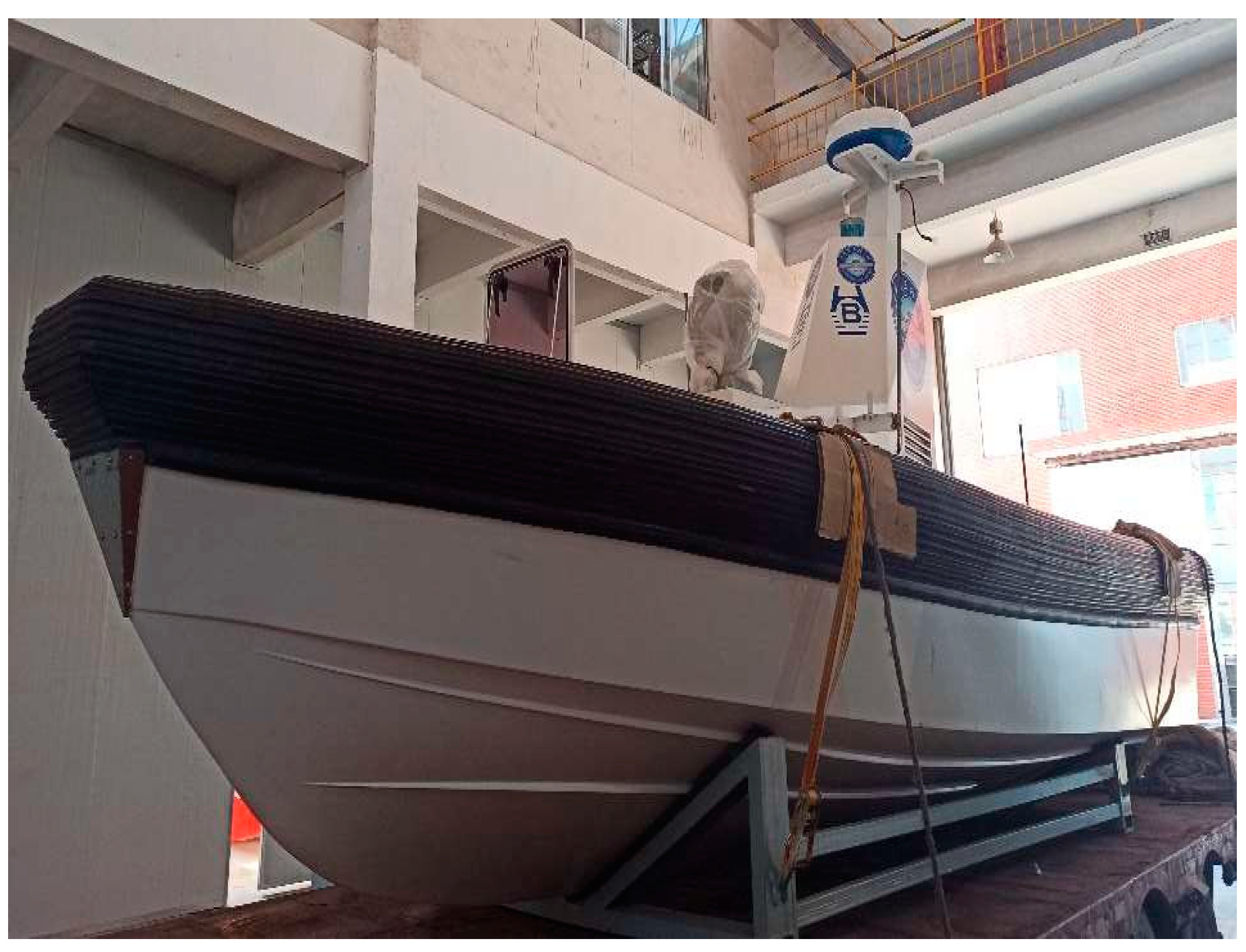
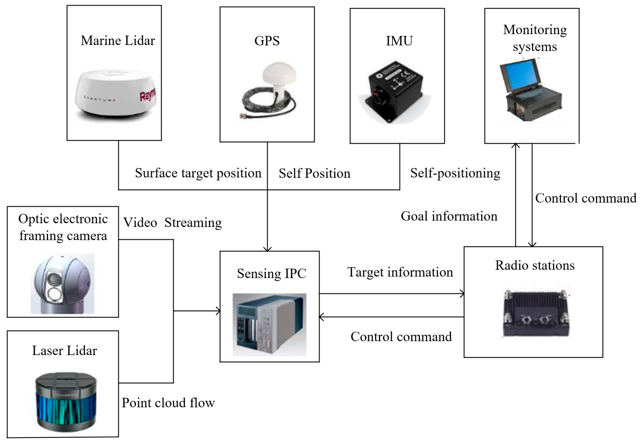
Figure 13 shows the "North Ocean" USV. The "North Ocean" USV platform sensing system used in this paper consists of a maritime lidar, a laser lidar, an optoelectronic camera, an inertial measurement unit (IMU), a global positioning system (GPS), and an industrial personal computer (IPC), as shown in
Figure 14. The sensing computer is equipped with an 8-core i7-7700T CPU and an NVIDIA RTX2080 GPU with 7981MB of memory.
The high-precision photoelectric video reconnaissance instrument, which is outfitted with a color CCD white light camera, is the apparatus used to acquire visible RGB images. This camera's maximum resolution is 1920 by 1080. It possesses the ability to output video images in the form of network encoding and automatically control the aperture.
4.3. Evaluation Metrics
In
Table 4, TP indicates the number of detection targets that are positive samples and are correctly detected at the same time; FP indicates the number of detection targets that are negative samples but are mistakenly detected as positive samples; FN indicates the number of detection targets that are positive samples but are mistakenly detected as negative samples; and TN indicates the number of detection targets that are negative samples and are correctly detected at the same time.
Precision (P) is defined as the number of positive samples detected correctly at the same time (TP) as a proportion of all positive samples detected; the higher the accuracy, the lower the probability of false detection of the target, so it is also called the accuracy. Recall (R) is defined as the number of positive samples detected correctly at the same time as the proportion of the total positive samples. The formulae for accuracy and recall are shown in Equations (11) and (12), respectively:
where
denotes the accuracy rate and
denotes the recall rate. The above formulae can be used to obtain the values of accuracy and recall at different thresholds, and the P-R curve is plotted. The area enclosed by the P-R curve and the coordinate axis is the average accuracy (AP), and its calculation formula is shown in Equations (13).
However, in practice, if integration is used to obtain the average accuracy, the steps are more cumbersome, so the interpolation sampling method is usually adopted to calculate the average value, and its calculation formula is shown in (14).
To examine the extent of model lightweight, the experiments will also use the number of parameters of the network model and the number of floating-point operations (GFLOPs), which are negatively correlated with the light weight of the model. The lighter the model, the lower these two parameters are, and the more favorable the model will be for deployment on USV.
4.4. Experimental Results and Analysis
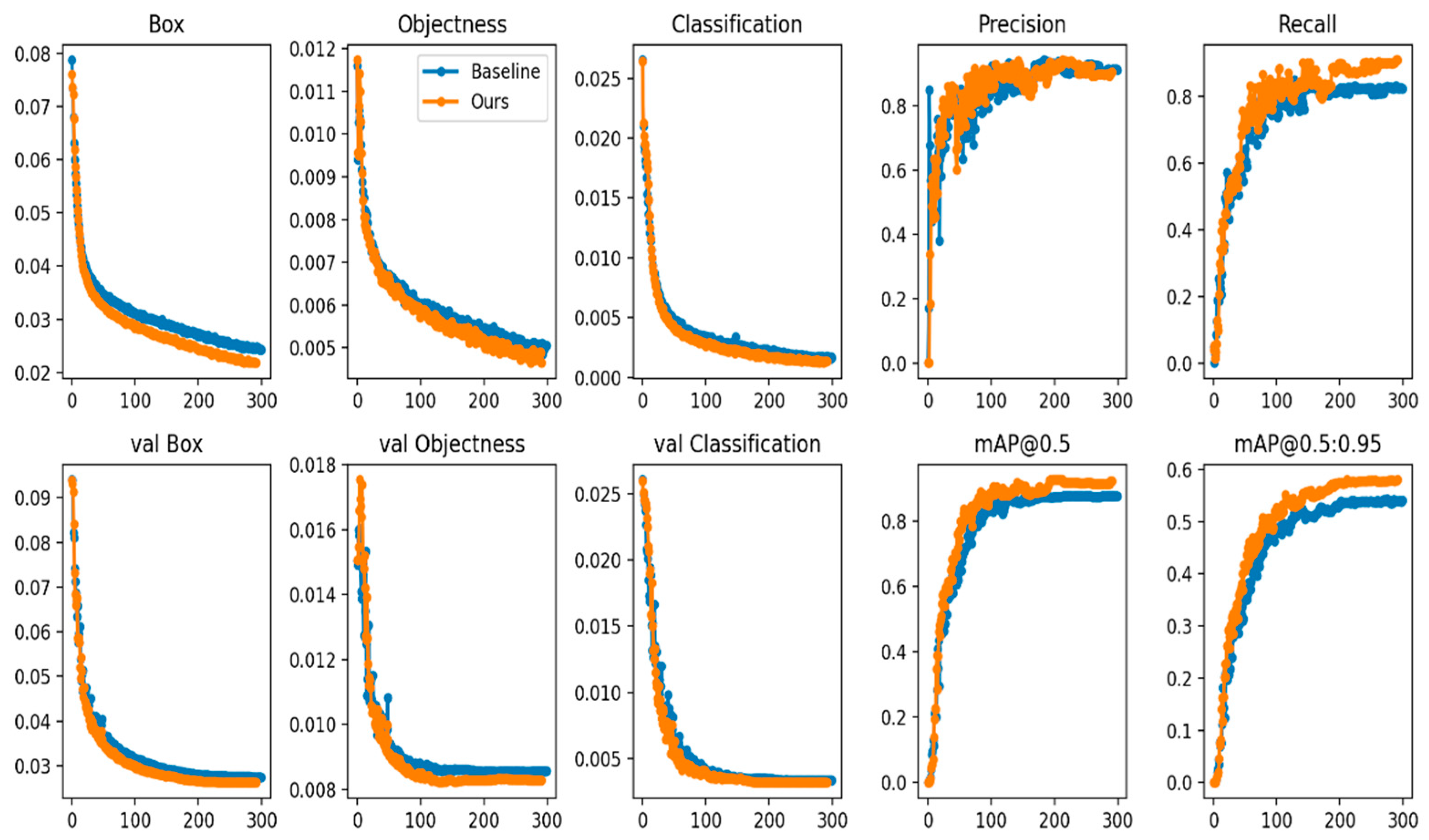
The training results and mAP metrics statistics are shown in
Table 5. The method in this paper shows an increase in mAP for each category of target compared to the base-line model.
Figure 15 displays the training's result curve. For the same 300 training epochs, the loss decreases more quickly. It is important to note that this strategy considerably raises the recall rate. Accordingly, our technique not only increases accuracy but also learns surface target properties more effectively, lowers the likelihood of missing a target detection, and identifies more targets in complex aquatic environments.
4.5. Comparison with Other Popular Models
To verify the superiority of the proposed model, this paper also compares it with other mainstream lightweight target detection models. In addition to the Yolo series models, this paper also refers to other lightweight models, such as Mobilenetv3 [
29], Ghostnetv2 [
30], Shufflenetv2 [
31], PP-PicoDet [
32], and FasterNet [
33], which are combined with Yolov7-tiny for comparison experiments. Considering its effectiveness, the platform used for the comparison is the industrial personal computer for the “North Ocean” USV platform. The experimental results are shown in
Table 6.
By contrasting several models, we can find that the accuracy and recall of the Yolov8 have the highest accuracy and recall, while the number of methodological parameters in this study is modest and only partially redundant. the model after combining GhostNet v2 that has the fewest GFLOPs. Although YOLOX-tiny has the fastest detection speed and the fewest parameters, its recall is substantially lower than that of the baseline model, making it useless for detecting targets on the water's surface. Although this method's mAP is substantially improved and its GFLOPs are slightly greater than other lightweight approaches, it is more effective at combining multi-scale water surface target features.Although the method in this paper does not have the advantage of speed, it fully satisfies the input requirement of 30 fps for the USV-equipped optoelectronic pods and can easily achieve real-time detection.
4.6. Ablation Experiments
The ablation experiments show that the network learning capability is effectively improved by replacing the LeakyReLU activation function with the Mish and SiLU activation functions. R2B improves accuracy by better integrating multi-scale features. R2B is lighter and more suitable for surface target detection than the original MCB, reducing the 1.22M parameters of the network model. The addition of CoordConv to Neck incorporates more feature information, and the increase in the number of parameters and computations is almost negligible. After using DyHead, the number of prediction channels is set to 128, which can effectively improve the accuracy while slightly reducing the parameters, but of course, it also brings some increase in inference time.
4.7. Comparative Analysis of Visualization Results
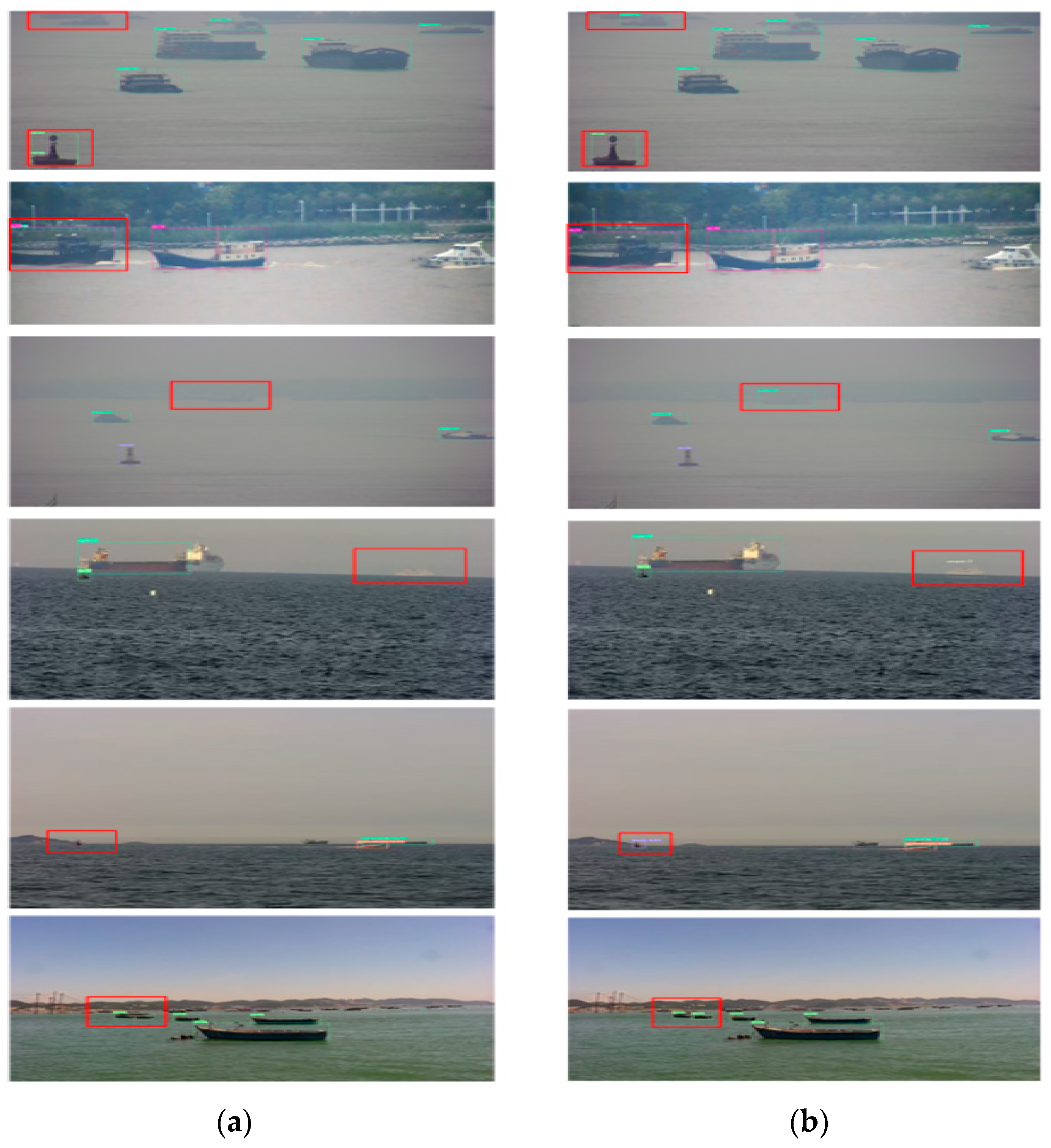
Some visualizations of the detection results on the test set are shown in
Figure 16. The method presented in this work is better able to learn multi-scale target features, as shown by the
Figure 16. For instance, angle fluctuations and intraclass variances have an impact on the detection of multi-scale ships with significant aspect ratio variations; however, this method is more successful in identifying and capturing the target information of the ship. Additionally, this approach works better in challenging aquatic conditions like foggy weather, overlapping targets, small targets, and light and darkness effects.
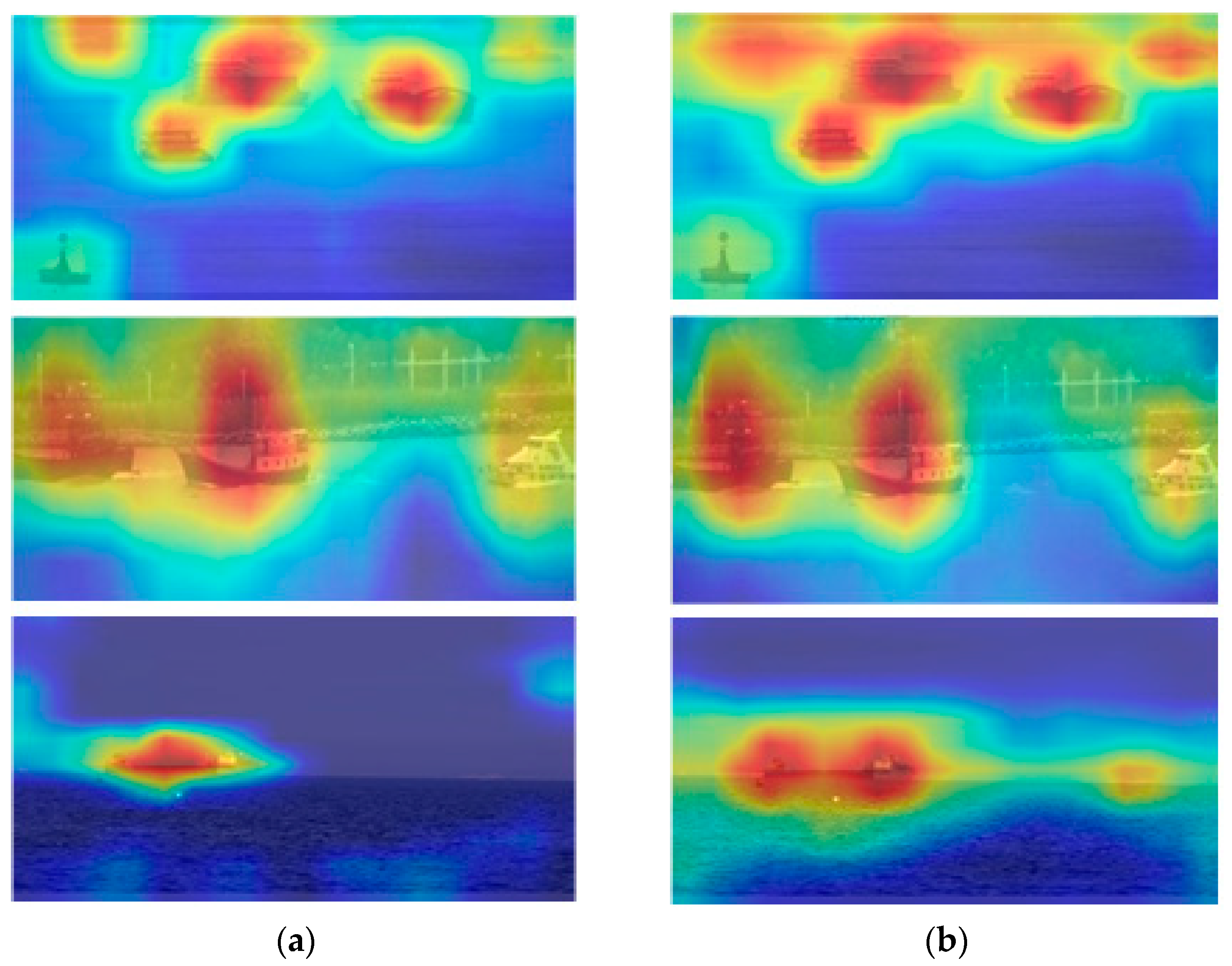
Figure 17 compares the deep network attention heat map of the detection outcomes. Our efficiently captures spatial information on the depth feature map. For instance, when determining the type of ship, the more reliable bow and stern structures are given more consideration than the intermediate hull. Additionally, it combines more environmental data and concentrates on targets that are easily missed. This image effectively illustrates how mindful attention may be used to learn from DyHead.
4.8. Experiments in Generalization Ability
Another Singapore Maritime Dataset (SMD) [
34] was prepared to validate the applicability of the model for multi-scene surface target detection tasks. SMD is a video dataset of sea scenes containing numerous multi-scale ship targets, with images taken on deck and ashore, mainly video continuous frame images. Its dataset is shown in
Figure 18 below. In this paper, a frame-drawing method is used to create a home-made dataset to validate the generalization capability of the model to different scenes.
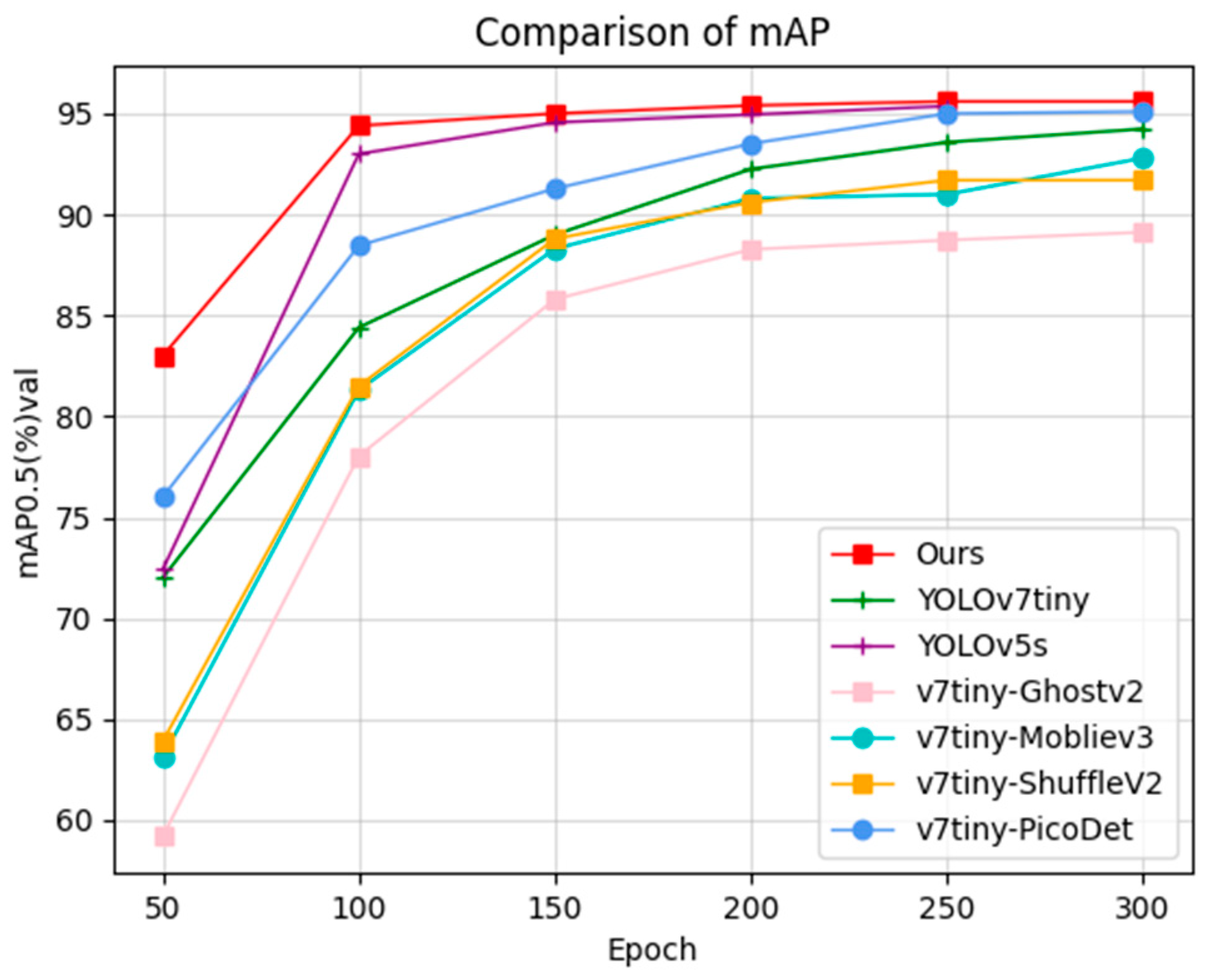
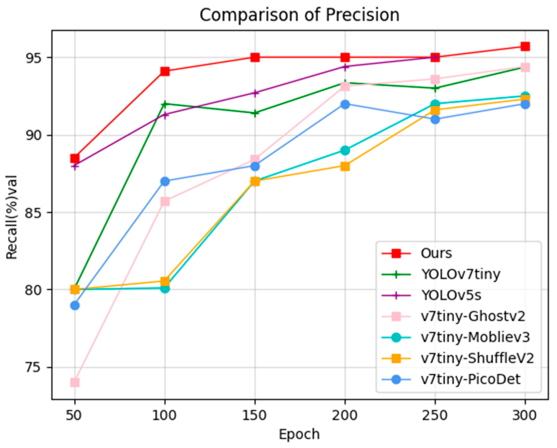
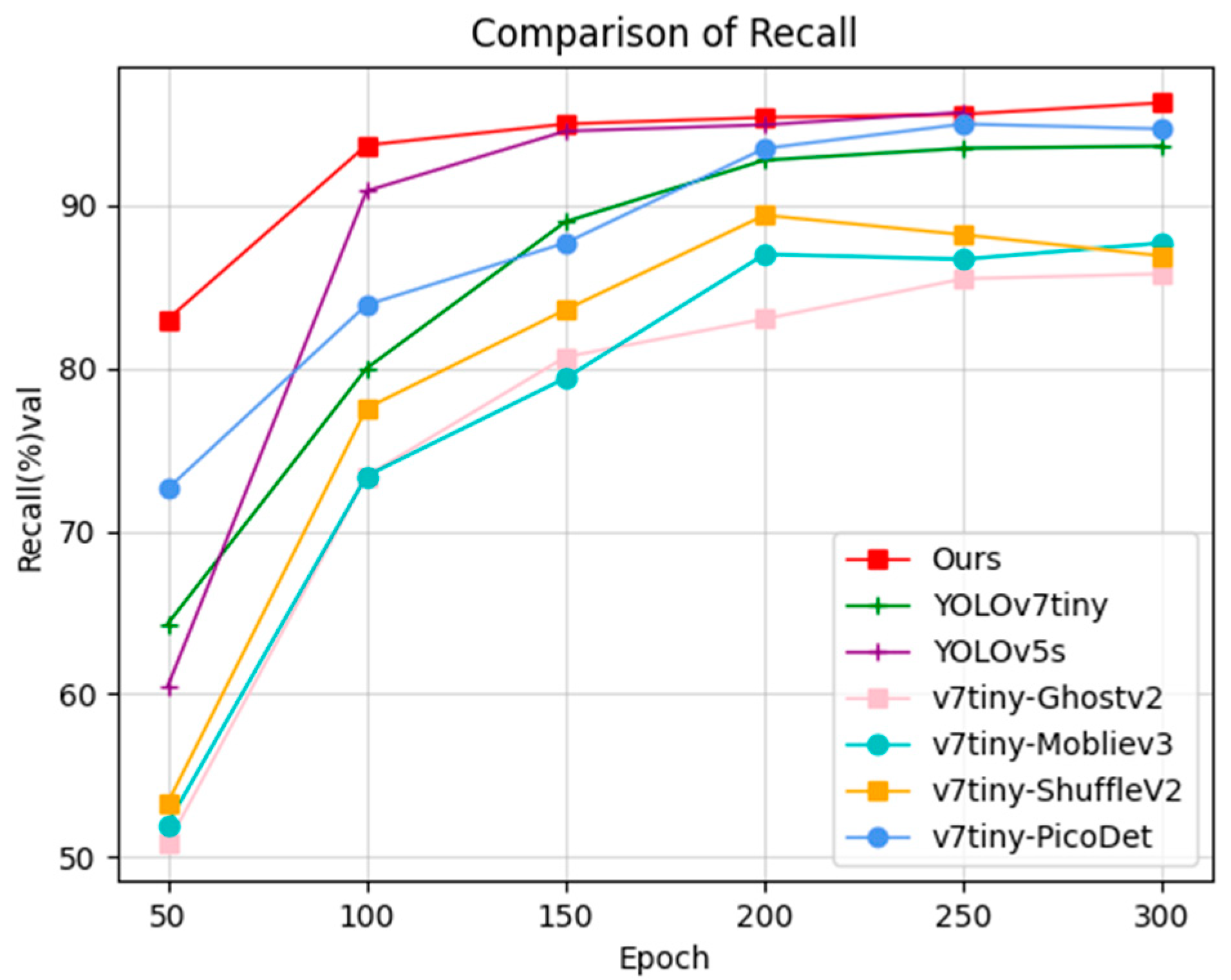
In this section, several models are also selected for comparative analysis. The experimental platform and parameters were kept consistent, and the results were compared across multiple models in the following
Figure 19,
Figure 20 and
Figure 21:
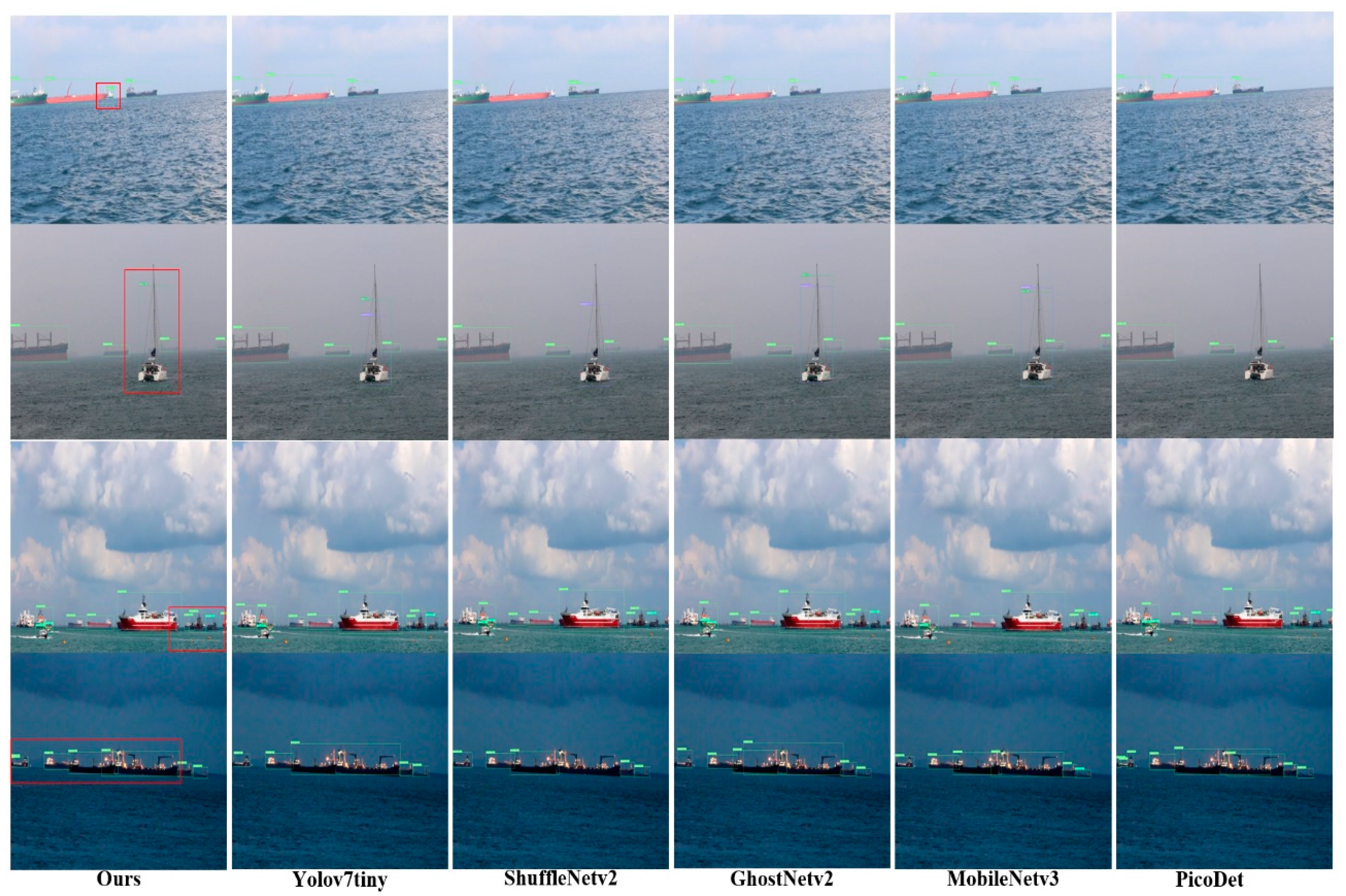
The line graphs show that ours and the YOLOv5s are the best in terms of SMD, with similar metrics in every aspect and both performing significantly better than the base model. The method presented in this study, however, is computationally challenging, converges more quickly, and has a limited number of parameters. When integrated with Pico-Det network work, the network also outperforms the baseline model, although the issue that the PicoDet model is too computationally expensive still exists.
Figure 22 displays the outcomes of the partial detection on the test set. The graph demonstrates that the strategy presented in this research works well in the new case as well. Compared to other lightweight approaches, the detection frame has fewer errors and misses and is more accurate. In conclusion, the method presented in this work is more broadly applicable than existing lightweight methods and is appropriate for a variety of applications.
5. Conclusions and Discussion
With the development of deep learning, more and more research has focused on the field of surface target detection. In this paper, a lightweight detection method for USV is investigated. The method of enhancing multi-scale feature fusion of surface targets is investigated while ensuring sufficient detection speed. Most previous studies have mostly used a combination of different lightweight convolutional approaches as well as attentional mechanisms, and these operations can significantly reduce detection accuracy. In this paper, we combine the characteristics of multi-scale water surface targets and focus on fusing more effective features with fewer convolution operations. Therefore, this paper investigates a method to improve accuracy while reducing the number of parameters and operations.
This paper presents a lightweight multi-scale feature-enhanced detection method for surface target detection on USV that can achieve a balance of efficiency and accuracy. Compared with the original Yolov7tiny model and other lightweight methods, it has obvious advantages in terms of missed and wrong detections in sophisticated scenes, combines accuracy and real-time performance, and is more suitable for water surface target detection. The generalization ability over the original model in different water scenarios also has a clear advantage. This paper also combines other lightweight methods and designs other improved models for comparative experiments, providing a valuable reference for the re-examination of USV lightweight detection.
Due to the constraints, no experiments were conducted for real detection missions. Future research should consider conducting sea trials to verify the practical effectiveness of the method. and further reduce the computational effort of the model, making it less demanding to deploy.
Author Contributions
Conceptualization, L.Z.; methodology, X.D.; software, X.D.; validation, L.Z., R.Z., and J.Z.; formal analysis, L.Z., and J.Z.; investigation, X.D.; resources, L.Z.; data curation, X.D.; writing—original draft preparation, X.D.; writing—review and editing, L.Z.; visualization, X.D.; supervision, L.Z.; project administration, L.Z.; All authors have read and agreed to the published version of the manuscript.
Funding
This research was funded by [Heilongjiang Provincial Excellent Youth Fund] grant number [YQ2021E013] and [The National Key Research and Development Program of China] grant number [2021YFC2803400].
Institutional Review Board Statement
Not applicable.
Conflicts of Interest
The authors declare no conflict of interest.
References
- Liu, Z.; Zhang, Y.; Yu, X.; Yuan, C. Unmanned surface vehicles: An overview of developments and challenges. Annual Re-views in Control. 2016, 41, 71–93. [Google Scholar] [CrossRef]
- Campbell, S.; Naeem, W.; Irwin, G. W. A review on improving the autonomy of unmanned surface vehicles through intel-ligent collision avoidance manoeuvres. Annual Reviews in Control. 2012, 36, 267–283. [Google Scholar] [CrossRef]
- Huang, B.; Zhou, B.; Zhang, S.; Zhu, C. Adaptive prescribed performance tracking control for underactuated autonomous underwater vehicles with input quantization. Ocean. Eng. 2021, 221, 108549. [Google Scholar] [CrossRef]
- Gao, J.; Zhang, J.; Liu, C.; Li, X.; Peng, Y. Camera-LiDAR Cross-Modality Fusion Water Segmentation for Unmanned Surface Vehicles. Journal of Marine Science and Engineering. 2022, 10, 744. [Google Scholar] [CrossRef]
- Wang, L.; Fan, S.; Liu, Y.; Li, Y.; Fei, C.; Liu, J.; Liu, B.; Dong, Y.; Liu, Z.; Zhao, X. A Review of Methods for Ship Detection with Electro-Optical Images in Marine Environments. Journal of Marine Science and Engineering. 2021, 9, 1408. [Google Scholar] [CrossRef]
- Girshick, R.; Donahue, J.; Darrell, T.; Malik, J. Rich Feature hierarchies for accurate object detection and semantic segmentation. In Proceedings of the IEEE conference on computer vision and pattern recognition; 2014. pp. 580–587.
- Girshick, Ross. Fast r-cnn. In Proceedings of the IEEE international conference on computer vision; 2015.pp. 1440-1448.
- Ren, S. Q.; He, K. M.; Girshick, R.; Sun, J. Faster R-CNN: Towards Real-Time Object Detection with Region Proposal Networks. Ieee T Pattern Anal. 2017, 39, 1137–1149. [Google Scholar] [CrossRef] [PubMed]
- Liu, W.; Anguelov, D.; Erhan, D.; Szegedy, C.; Reed, S.; Fu, C. Y.; Berg, A. C. Ssd: Single shot multibox detector. Computer Vision – ECCV 2016: 14th European Conference, Amsterdam, The Netherlands, October 11–14, 2016, Proceedings, Part I 14. Springer International Publishing; 2016. pp. 21-37. 11 October.
- Liu, K.; Tang, H.; He, S.; Yu, Q.; Xiong, Y.; Wang, N. Performance validation of YOLO variants for object detection. In Proceedings of the 2021 International Conference on bioinformatics and intelligent computing; 2021. pp. 239–243.
- Redmon, J.; Divvala, S.; Girshick, R.; Farhadi, A. You only look once: Unified, real-time object detection. In Proceedings of the IEEE conference on computer vision and pattern recognition; 2016; pp. 779–788. [Google Scholar]
- Li, Y.; Guo, J.; Guo, X.; Liu, K.; Zhao, W.; Luo, Y.; Wang, Z. A novel target detection method of the unmanned surface vehicle under all-weather conditions with an improved YOLOV3. Sensors 2020, 20, 4885. [Google Scholar] [CrossRef]
- Zhu, X.; Lyu, S.; Wang, X.; Zhao, Q. TPH-YOLOv5: Improved YOLOv5 based on transformer prediction head for object detection on drone-captured scenarios. In Proceedings of the IEEE/CVF international conference on computer vision. 2021; pp. 2778–2788. [CrossRef]
- Wang, C. Y.; Bochkovskiy, A.; Liao, H. Y. M. YOLOv7: Trainable bag-of-freebies sets new state-of-the-art for real-time object detectors. arXiv 2022, arXiv:2207.02696. [Google Scholar]
- Martinez-Carranza, J.; Hernandez-Farias, D. I.; Rojas-Perez, L. O.; Cabrera-Ponce, A. A. Language meets YOLOv8 for metric monocular SLAM. Journal of Real-Time Image Processing. 2023, 20, 222–227. [Google Scholar] [CrossRef]
- Yang, Z.; Li, Y.; Wang, B.; Ding, S.; Jiang, P. A Lightweight Sea Surface Object Detection Network for Unmanned Surface Vehicles. Journal of Marine Science and Engineering. 2022, 10, 965. [Google Scholar] [CrossRef]
- Liu, T.; Pang, B.; Zhang, L.; Yang, W.; Sun, X. Sea Surface Object Detection Algorithm Based on YOLO v4 Fused with Reverse Depthwise Separable Convolution (RDSC) for USV. Journal of Marine Science and Engineering. 2021, 9, 753. [Google Scholar] [CrossRef]
- Wang, Y.; Li, J.; Tia, Z.; Chen, Z.; Fu, H., Ship Target Detection Algorithm Based on Improved YOLOX_s. In 2022 IEEE International Conference on Mechatronics and Automation (ICMA), 2022; pp. 1147-1152.
- Ma, R. X.; Bao, K. X.; Yin, Y. , Improved Ship Object Detection in Low-Illumination Environments Using RetinaMFANet. J Mar Sci Eng 2022, 10, 1996. [Google Scholar] [CrossRef]
- Wang, B.; Han, B.; Yang, L., Accurate Real-time Ship Target detection Using Yolov4. In 2021 6th International Conference on Transportation Information and Safety (ICTIS), 2021; pp 222-227.
- He K., Zhang X., Ren S., Sun J., Delving deep into rectifiers: Surpassing human-level performance on imagenet classification. In Proceedings of the IEEE International Conference on Computer Vision (ICCV), 2015; pp. 1026-1034.
- Misra, D. Mish: A self regularized non-monotonic activation function. arXiv 2020, arXiv:1908.08681. [Google Scholar]
- Ramachandran, P.; Zoph, B.; Le, Q. V. Searching for activation functions. arXiv 2017, arXiv:1710.05941. [Google Scholar]
- Gao, S. H.; Cheng, M. M.; Zhao, K.; Zhang, X. Y.; Yang, M. H.; Torr, P. , Res2Net: A New Multi-Scale Backbone Architecture. Ieee T Pattern Anal 2021, 43, 652–662. [Google Scholar] [CrossRef]
- Liu, R.; Lehman, J.; Molino, P.; Such, F. P.; Frank, E.; Sergeev, A.; Yosinski, J. An intriguing failing of convolutional neural networks and the CoordConv solution. Adv Neur In 2018, 31. [Google Scholar]
- Dai, X. Y.; Chen, Y. P.; Xiao, B.; Chen, D. D.; Liu, M. C.; Yuan, L.; Zhang, L. Dynamic Head: Unifying Object Detection Heads with Attentions. Proc Cvpr Ieee 2021, 7369–7378. [Google Scholar]
- Shao, Z. F.; Wu, W. J.; Wang, Z. Y.; Du, W.; Li, C. Y. SeaShips: A Large-Scale Precisely Annotated Dataset for Ship Detection. Ieee T Multimedia 2018, 20, 2593–2604. [Google Scholar] [CrossRef]
- Zhou, Z. G.; Sun, J. E.; Yu, J. B.; Liu, K. Y.; Duan, J. W.; Chen, L.; Chen, C. L. P. An Image-Based Benchmark Dataset and a Novel Object Detector for Water Surface Object Detection. Front Neurorobotics 2021, 15. [Google Scholar] [CrossRef] [PubMed]
- Howard, A.; Sandler, M.; Chu, G.; Chen, L. C.; Chen, B.; Tan, M. X.; Wang, W. J.; Zhu, Y. K.; Pang, R. M.; Vasudevan, V.; Le, Q. V.; Adam, H. Searching for MobileNetV3. Ieee I Conf Comp Vis 2019, 1314–1324. [Google Scholar] [CrossRef]
- Tang, Y. H.; Han, K.; Guo, G. Y.; Xu, C.; Xu, C.; Wang, M. X.; Wang, Y. H. GhostNetV2: Enhance Cheap Operation with Long-Range Attention. arXiv 2022, arXiv:2211.12905. [Google Scholar]
- Ma, N. N.; Zhang, X. Y.; Zheng, H. T.; Sun, J. ShuffleNet V2: Practical Guidelines for Efficient CNN Architecture Design. Lect Notes Comput Sc 2018, 11218, 122–138. [Google Scholar] [CrossRef]
- Yu, G. H.; Chang, Q. Y.; Lv, W. Y.; Cui, C.; Ji, W.; Dang, M. X.; Wang, Q. Q. PP-PicoDet: A Better Real-Time Object Detector on Mobile Devices. arXiv 2021, arXiv:2111.00902. [Google Scholar]
- Chen, J. R.; Kao, S. H.; He, H.; Zhuo, W, P.; Wen, S.; Lee, C. H. Run, Don’t Walk: Chasing Higher FLOPS for Faster Neural Networks. arXiv 2023, arXiv: 2303.03667.
- Prasad, D. K.; Rajan, D.; Rachmawati, L.; Rajabally, E.; Quek, C. Video Processing From Electro-Optical Sensors for Object Detection and Tracking in a Maritime Environment: A Survey. Ieee T Intell Transp 2017, 18, 1993–2016. [Google Scholar] [CrossRef]
Figure 1.
Structure diagram of the YOLOv7-tiny.
Figure 1.
Structure diagram of the YOLOv7-tiny.
Figure 2.
Detailed view of the YOLOv7-tiny modules.
Figure 2.
Detailed view of the YOLOv7-tiny modules.
Figure 3.
Comparison of three activation functions.
Figure 3.
Comparison of three activation functions.
Figure 4.
Structure diagram of MCB-SM.
Figure 4.
Structure diagram of MCB-SM.
Figure 5.
Comparison of different structure. (a) Bottleneck; (b) Res2Net.
Figure 5.
Comparison of different structure. (a) Bottleneck; (b) Res2Net.
Figure 6.
Structure diagram of R2B.
Figure 6.
Structure diagram of R2B.
Figure 7.
Comparison of convolution methods. (a): normal convolution; (b): CoordConv.
Figure 7.
Comparison of convolution methods. (a): normal convolution; (b): CoordConv.
Figure 8.
An illustration of our Dynamic Head approach.
Figure 8.
An illustration of our Dynamic Head approach.
Figure 9.
The detailed configuration of Dynamic Head.
Figure 9.
The detailed configuration of Dynamic Head.
Figure 10.
Structure diagram of the YOLOv7-RCD model.
Figure 10.
Structure diagram of the YOLOv7-RCD model.
Figure 11.
Detailed view of the YOLOv7-RCD modules.
Figure 11.
Detailed view of the YOLOv7-RCD modules.
Figure 12.
Samples from our dataset.
Figure 12.
Samples from our dataset.
Figure 13.
The “North Ocean” USV platform.
Figure 13.
The “North Ocean” USV platform.
Figure 14.
Hardware structure diagram of the sensing system of the “North Ocean” USV platform.
Figure 14.
Hardware structure diagram of the sensing system of the “North Ocean” USV platform.
Figure 15.
Comparison of visual graphs of the training process.
Figure 15.
Comparison of visual graphs of the training process.
Figure 16.
Comparison of visualization detection results. (a): Baseline; (b): Ours.
Figure 16.
Comparison of visualization detection results. (a): Baseline; (b): Ours.
Figure 17.
Comparison of the deep attention heat map. (a): Baseline; (b): Ours combines a variety of conscious attention.
Figure 17.
Comparison of the deep attention heat map. (a): Baseline; (b): Ours combines a variety of conscious attention.
Figure 18.
Samples from the SMD.
Figure 18.
Samples from the SMD.
Figure 19.
Comparison of the map on SMD.
Figure 19.
Comparison of the map on SMD.
Figure 20.
Comparison of the precision on SMD.
Figure 20.
Comparison of the precision on SMD.
Figure 21.
Comparison of the recall on SMD.
Figure 21.
Comparison of the recall on SMD.
Figure 22.
Comparison of the detection results of different models in the test set.
Figure 22.
Comparison of the detection results of different models in the test set.
Table 1.
Experimental configuration.
Table 1.
Experimental configuration.
| Items |
Type |
| operating system |
Ubuntu 22.04 |
| programming Language |
Python 3.9 |
| deep learning framework |
Torch 2.0 CUDA11.8、cudnn8.8 |
| CPU |
Intel i5 9600K 3.7GHz 6 core |
| GPU |
RTX2080 8G |
Table 2.
Experimental Parameter Setting.
Table 2.
Experimental Parameter Setting.
| Parameter |
Configuration |
| learning rate |
0.01 |
| momentum |
0.937 |
| weight decay |
0.0005 |
| batch size |
32 |
| optimizer |
SGD |
| image size |
640×640 |
| epochs |
300 |
Table 3.
The instances information statistics of our dataset.
Table 3.
The instances information statistics of our dataset.
| Class |
Instances/Percentage% |
| boat |
1764/17.36 |
| cargo ship |
4620/45.48 |
| passenger ship |
790/7.78 |
| speed boat |
753/7.41 |
| ship |
1724/16.9 |
| buoy |
506/5.0 |
Table 4.
Model evaluation metrics.
Table 4.
Model evaluation metrics.
| Confusion Matrix |
Predicted value |
Ground Truth
True
False |
Positive |
Negative |
| TP |
FN |
| FP |
TN |
Table 5.
Comparison of mAP before and after improvement.
Table 5.
Comparison of mAP before and after improvement.
| Class |
mAP@.5 Ours/Baseline% |
mAP@.5:.95 Ours/Baseline% |
| all |
92.85/86.67 |
58.7%/54.3% |
| boat |
81.8/77.7 |
42.6/38.2 |
| cargo ship |
98.4/94.1 |
72.1/68.6 |
| passenger ship |
94.9/91.1 |
70.8/67.9 |
| speed boat |
95.2/83.1 |
48.5/41.2 |
| ship |
96.3/92.1 |
63.3/60.8 |
| buoy |
90.5/81.9 |
54.9/49.1 |
Table 6.
Comparison of popular models on the sensing IPC for USV.
Table 6.
Comparison of popular models on the sensing IPC for USV.
| Model |
Param (M) |
GFLOPs |
Precision% |
Recall% |
mAP@.5% |
mAP@.5:.95% |
FPS |
| SSD |
41.1 |
387.0 |
80.46 |
71.37 |
77.46 |
47.93 |
24.84 |
| YOLOv4-tiny |
6.05 |
13.7 |
77.23 |
69.26 |
70.35 |
39.66 |
75.64 |
| YOLOv5s |
7.06 |
15.9 |
88.12 |
83.31 |
87.66 |
53.92 |
55.52 |
| YOLOX-tiny |
5.10 |
6.51 |
83.23 |
81.62 |
81.56 |
50.23 |
75.97 |
| YOLOv8-tiny |
3.01 |
8.1 |
85.3 |
81.1 |
85.46 |
52.69 |
72.64 |
| YOLOv7-tiny-ShuffleNetv2 |
5.66 |
9.2 |
85.8 |
78.24 |
84.71 |
50.24 |
63.44 |
| YOLOv7-tiny-PicoDet |
4.76 |
29.4 |
79.33 |
84.41 |
86.41 |
52.88 |
60.11 |
| YOLOv7-tiny-GhostNetv2 |
5.84 |
5.31 |
89.51 |
75.4 |
84.92 |
48.01 |
66.82 |
| YOLOv7-tiny-MobileNetv3 |
4.86 |
7.52 |
80.2 |
79.4 |
84.2 |
51.1 |
65.69 |
| YOLOv7-tiny-FasterNet |
3.61 |
7.3 |
85.9 |
82.8 |
87.34 |
52.33 |
70.24 |
| YOLOv7-tiny |
6.02 |
13.2 |
90.42 |
82.8 |
86.73 |
54.47 |
68.79 |
| YOLOv7-RCD |
4.69 |
11.2 |
91.57 |
90.23 |
92.85 |
58.7 |
56.87 |
Table 7.
The results of ablation experiments.
Table 7.
The results of ablation experiments.
| Model |
Param(M) |
GFLOPs |
mAP@.5% |
mAP@.5:.95% |
| base |
6.02 |
13.2 |
86.73 |
54.47 |
| base+Mish |
6.02 |
13.2 |
87.33 |
54.93 |
| base+Mish+SiLu |
6.02 |
13.2 |
88.56 |
55.82 |
| base+Mish+SiLu+R2B |
4.8 |
11.2 |
90.29 |
57.43 |
| base+Mish+SiLu+ CoordConv |
4.8 |
11.2 |
91.09 |
57.91 |
| base+R2B+SiLu+Mish+CoordConv+DyHead |
4.69 |
11.2 |
92.83 |
58.71 |
|
Disclaimer/Publisher’s Note: The statements, opinions and data contained in all publications are solely those of the individual author(s) and contributor(s) and not of MDPI and/or the editor(s). MDPI and/or the editor(s) disclaim responsibility for any injury to people or property resulting from any ideas, methods, instructions or products referred to in the content. |
© 2023 by the authors. Licensee MDPI, Basel, Switzerland. This article is an open access article distributed under the terms and conditions of the Creative Commons Attribution (CC BY) license (http://creativecommons.org/licenses/by/4.0/).
