Preprint
Article

Effects of a Late Gravitational Transition on Gravitational Waves and Anticipated Constraints

Altmetrics

Downloads

128

Views

51

Comments

0

A peer-reviewed article of this preprint also exists.

Submitted:

12 June 2023

Posted:

12 June 2023

You are already at the latest version

Alerts
Abstract
We investigate the evolution of gravitational waves through discontinuous evolution (transition) of the Hubble expansion rate H(z) at a sudden cosmological singularity which may be due to a transition of the value of the gravitational constant. We find the evolution of the scale factor and the gravitational wave waveform through the singularity by imposing the proper boundary conditions. We also use existing cosmological data and mock data of future gravitational wave experiments (the ET) to impose current and anticipated constraints on the magnitude of such a transition. We show that mock data of the Einstein Telescope can reduce the uncertainties by up to a factor of 3 depending on the cosmological parameter considered.
Keywords: 
Subject: Physical Sciences  -   Astronomy and Astrophysics

1. Introduction

The standard cosmological model ( Λ CDM) [1,2,3,4,5,6,7] provides a good fit to a wide range of cosmological data despite its relatively small number of parameters. However, some important parameters of the model like the Hubble parameter H 0 and parameters related to the growth rate of cosmological perturbations appear to have conflicting best fit values depending on the type of cosmological observations used for their estimation (For a review [8]). Thus there are tensions among the best fit values of Λ CDM cosmological parameters. The most important such tension is the Hubble tension at a level of 5 σ [9]. In particular, P l a n c k 2018 CMB measurements and BAO measurements (if combined) give a best fit value for the Hubble parameter H 0 = ( 67.4 ± 0.5 ) k m s M p c [1], while "local" measurements using mainly type Ia supernovae as standard candles[10], give a best fit value for the Hubble flow H 0 = ( 73.04 ± 1.04 ) k m s M p c [8,9,11]. A wide range of extensions of Λ CDM has been implmeneted to address this tension. These approaches may be divided in three categories
  • Early time models[12,13,14,15,16] (see also [17] for a review) that implement new degrees of freedom (eg Early Dark energy [12,13,14,18], New Early Dark Energy[15,16] etc) to decrease the scale of the sound horizon at recombination. This scale can be used as a standard ruler to measure the Hubble parameter [19,20] after calibration from the CMB angular power spectrum peak locations[1]. These models however have two problems: 1. They require significant fine tuning in order to avoid conflict with cosmological observations after the time of recombination [21,22] and 2. They should also decrease the horizon scale at the time of equal time matter and radiation density which can also be calibrated using the matter power spectrum [23,24].
  • Late time models [25,26,27,28,29,30,31,32,33] that attempt to deform the Planck 18 best fit Λ CDM form of Hubble free expansion rate E ( z ) H ( z ) / H 0 between the time of recombination and the present time so that the present time value H ( z = 0 ) becomes consistent with the SH0ES best fit value[10]. The problem of this class of models is that the significant level of E ( z ) deformation needed, is not consistent with a wide range of other observations constraining the form of E ( z ) like BAO and SnIa data [34,35,36,37].
  • Ultra late time models [36,38,39,40,41,42] that investigate the possible presence of either an unaccounted for systematic effect and/or a change of fundamental physics taking place during the last 150 M y r s (redshift z < 0.01 ) when the calibration of standard candles like SnIa is performed [11]. The problems of this class of models includes fine tuning since the change of physical laws should not only have at very late times but also it should be consistent with other local observations[43].
In the context of ultralate time models [11,41,43,44] there is an abrupt transition of the SnIa absolute luminosity and/or of their calibrators (eg Cepheids and TRGB [44]) which becomes realized at a specific distance d c [ 10 , 60 ] M p c due to either a physics transition taking place globally in the Universe during the last 150 M y r s or locally in our local Universe within distances smaller than 60 M p c . A smoking gun prediction of this class of models is a sudden change of the SnIa absolute magnitude at a distance d c < 60 M p c . Recent analyses have indicated hints for hidden signals in the SH0ES [11] and Pantheon+ SnIa data which are consistent with such a transition [40]. A physical mechanism for the realization of such a transition includes an explicit symmetry breaking in the context of the symmetron screening mechanism (the asymmetron [45]) as well as a first order phase transition in the context of a scalar-tensor theory [46]. In the context of such mechanism it would be expected that the Hubble expansion rate H ( z ) could also receive a step-like discontinuity due to the anticipated transition. Such a transition however would be difficult to observe in the context of SnIa standard candle probes of H ( z ) due to the peculiar velocity noise that prohibits the precise measurement of H ( z ) at redshifts z < 0.01 . However, it is still possible to investigate anticipated constraints on such a physics transition using forthcoming gravitational wave data and existing cosmological data. This is the goal of the present analysis.
We thus impose constraints on a transition in the value of effective gravitational constant G eff which would induce a sudden change of the Hubble flow rate. If such a change is advocated through a phenomenological parametrization of the form H ( t ) [ 1 + σ Θ ( t t s ) ] , where σ is a dimensionless parameter and Θ is the Heavyside step function, then it is deemed to exhibit the characteristics of a sudden cosmological singularity[47,48,49,50,51,52]. For instance, in sudden cosmological singularities or type II, at the time t = t s we have divergence of pressure t = t s | p ( t s ) | with finite density ρ ( t s ) < and scale factor a ( t s ) < , while the scale factor is continuous at t s [47,49,51,53]. The Hubble flow is finite, or H ( t s ) < , but the derivative of its diverge, or H ˙ ( t s ) . In this case, the divergence of pressure leads to violation of the dominant energy condition [54]. A geodesically complete singularity (like the sudden cosmological singularity [49,51,52]) involves a divergence of a derivative of the scale factor while a 0 and a < through the moment which occurs.
In this paradigm, the generalized sudden cosmological singularities can be considered [55], where the order-r derivative of the scale factor diverges, leading to divergence of the corresponding r 1 derivative of pressure. Our universe could confront a sudden singularity at the near future, that would not be the "end" of it [56] and could even mimic at the present day standard dark energy models [56].
Extensions of Λ CDM predict the existence of a wide range of singularities [57,58]. These include the Big Rip singularities or Type I[59,60] where at a finite cosmic time, the scale factor, the Hubble flow, energy density and pressure diverge. For these singularities there is geodesic incompleteness, except for some values of the barotropic index w for which there is null geodesic completeness[51]. The type III-IV singularities involve a finite scale factor at the moment of the singularity or a ( t s ) < . Type III singularities (or finite scale factor singularity) [61,62] endure that ρ ( t s ) , | p ( t s ) | in finite cosmic time while the scale factor is discontinuous at t s , and also type IV singularities[60] admit that ρ ( t s ) = 0 , | p ( t s ) | = 0 and the barotropic index, the first derivative of pressure, the second, of Hubble flow and the third of scale factor diverge. Other singularities include w-singularities ( p ( t s ) = ρ ( t s ) = 0 while w ( t s ) ) [63], the Little-Rip (all the bound structures dissociate when a ( t s ) , ρ ( t s ) while t s )[64] and the Pseudo-Rip (all the bound structures below a corresponding threshold dissociate when H ( t s ) = c o s n t . while t s )[65].
A measure of the strength of a singularity is the strong curvature criterion by Krolak[66], which measures the time integrals of the tidal forces along geodesics [52] obtained by Krolak integral [52,66]: 0 τ | R i 0 j 0 ( τ ) | d τ where τ is the affine parameter along the geodesic. A causal geodesic hits to a strong curvature singularity by Krolak[66], for some value τ s of the affine parameter iff by taking the limit τ τ s the integral 0 τ | R i 0 j 0 ( τ ) | d τ diverges 1 [49,51,52,68].
A geodesically complete singularity could be induced by a rapid transition of the effective gravitational constant. Such a transition is motivated by the ultralate time models for the resolution of the Hubble tension. It could also help resolve the growth tension as it would reduce the growth of density perturbations without affecting the Planck / Λ CDM background expansion [38,41,45]. An abrupt shift of G eff is weakly constrained and the current bounds allow an abrupt change of G eff by up to about 5-10 % at some cosmological time in the past between the present time and the time of nucleosynthesis[45]. This is demonstrated in Table 1[41] where we show some current constraints on an overall change of G eff .
Since H 2 ( z ) G eff ( z ) , a sudden change of G eff ( z ) would be connected with a transition of the Hubble expansion rate H ( z ) thus leaving interesting signatures in cosmological data. The goal of the present analysis is to identify these signatures in present and future data and impose constraint in the amplitude and redshift of such a transition from anticipated gravitational wave data from the Einstein Telescope (ET) [75,76,77,78,79,80,81,82] and from other existing data including the Pantheon+ dataset and BAO-CMB data.
The structure of this paper is the following: In the next section we discuss some theoretical models that could induce such a gravitational transition in the context of scalar-tensor theories. In addition, we discuss the effects of an evolving G eff on the propagation of gravitational waves with emphasis on the particular evolution corresponding to an abrupt transition. In Section 3.1 we construct mock data based on the anticipated ET[75,77,78,80] which is third-generation ground-based gravitational wave observatory, designed to significantly improve the sensitivity and frequency range compared to the current second-generation detectors [83], such as LIGO [84] Virgo [85], and KAGRA [86]. We then use these data to derive the anticipated level of constraints to be imposed by these data on the amplitude of a gravitational transition. In Section 3.2 and Section 3.3 we focus on existing SnIa, BAO and CMB data to impose constraints on such a gravitational transition. We also discuss the anticipated improvement of these constraints in the context of the ET data at Section 3.4. Finally in Section 4 we conclude summarize and discuss possible future extensions of our analysis.

2. Evolving gravitational constant and gravitational waves in a cosmological background

2.1. Effective gravitational strength in scalar tensor theories with a gravitational transition

A natural theoretical setup for the realization of evolution of the strength of gravity includes scalar tensor gravitational theories. These modified gravity theories, are based on the metric g μ ν and a scalar field Φ directly coupled to the Ricci scalar R[17,87]. Thus, the gravitational interaction is mediated by both the metric tensor g μ ν , the scalar field Φ and an arbitrary coupling which determine the relative strength of the scalar field. The Lagrangian density is written as
L = 1 2 F ( Φ ) R g μ ν μ Φ ν Φ U ( Φ ) + L m a t t e r
in the Jordan frame[88], where F ( Φ ) is the dimensionless nonminimal coupling function of the scalar field Φ , U ( Φ ) is the corresponding potentilal and L m a t t e r depends on the metric and on the matter fields (coupled to the metric). In these theories the strength of gravity is determined by the effective gravitational constant
G eff G N = 1 F ( Φ ) 2 F ( Φ ) + 4 ( d F ( Φ ) d Φ ) 2 2 F ( Φ ) + 3 ( d F ( Φ ) d Φ ) 2
where G N is the value of Newton’s constant in the context of General Relativity. We define G * ( Φ ) G N F ( Φ ) . This is the inverse of the Planck mass squared M * 2 = G * 1 [88] and it appears in the Friedmann equations. We now consider a gravitational strength transition taking place at a redshift z s , in a flat universe, leading to a sudden change of the strength of gravity
G eff G N = 1 + α Θ [ z ( Φ ) z s ]
This assumption leads to a discontinous nonminimal coupling function
F 1 ( Φ ) = 1 + α Θ [ z ( Φ ) z s ]
and thus to a discontinuous Hubble expansion rate
H 2 H 0 2 = [ 1 + α Θ ( z z s ) ] [ 1 Ω m , 0 + Ω m , 0 ( 1 + z ) 3 ]
Using this information about F ( Φ ) , it is straightforward to reconstruct the redshift dependence of Φ ( z ) and U ( z ) using the reconstruction approach of Refs [88,89,90] leading to
U ( z ) = 3 ( 1 Ω m , 0 ) [ 1 + Δ 0 ( α ) δ ( z z s ) ]
Φ ( z ) = Φ 0 [ 1 + Δ 1 ( α ) Θ ( z z s ) ]
where Δ 0 ( α ) and Δ 1 ( α ) , are proper functions of α . Thus in this context, it is spike feature of the potential that can lead to a sudden change of the value of the scalar field Φ is the context of a flat potential. A similar effect would be induced in the context of a first order phase transition involving a decay of a false vacuum of the scalar field potential.

2.2. Luminosity distance from gravitational waves in modified gravity

In modified gravity theories, the luminosity distance as measured with gravitational waves may deviate from the standard general relativistic case due to several factors (see [91,92]):
  • Modifications to the cosmological expansion history: Some modified gravity theories predict a different cosmic expansion history compared to general relativity, which can lead to changes in the luminosity distance-redshift relationship. As a result, the measured luminosity distance using gravitational waves may differ in these theories [93].
  • Additional gravitational wave polarization modes: In some modified gravity theories, gravitational waves can have additional polarization modes [94], such as scalar or vector modes, in addition to the standard tensor modes found in general relativity. The presence of these additional modes can affect the amplitude and phase evolution of the gravitational wave signal, leading to a different measured luminosity distance.
  • Propagation effects: The propagation of gravitational waves in modified gravity theories can be affected by changes in the effective gravitational constant or the presence of additional fields. These effects can alter the gravitational wave amplitude and, consequently, the inferred luminosity distance[91,95].
By comparing the luminosity distance measurements obtained from gravitational waves with those obtained from electromagnetic observations, such as Type Ia supernovae or galaxy surveys, it is possible to test and constrain modified gravity theories[96,97]. Any significant discrepancy between the two sets of measurements could provide evidence for deviations from general relativity and help identify the correct gravitational theory.
The luminosity distance in general relativity plays a crucial role in determining the relationship between the intrinsic luminosity of an astrophysical source and its observed flux. For both electromagnetic and gravitational wave signals, the amplitude of the signal is expected to decay inversely with the luminosity distance. In general relativity, the electromagnetic and gravitational wave luminosity distances are the same, as they both depend in the same way on the underlying cosmological model[96,97].
However, in some modified gravity theories, the effective gravitational constant G eff can evolve with time or cosmic redshift z. This can lead to a difference in the propagation of gravitational waves compared to electromagnetic waves, and thus, a difference in the luminosity distances[93].
To derive the relation between the gravitational wave and electromagnetic luminosity distances, we can use the following assumptions:
  • The energy carried by gravitational waves is proportional to the square of the amplitude of the wave, which in turn, is proportional to the time-varying effective gravitational constant G eff ( z ) .
  • The energy carried by electromagnetic waves is not affected by the time-varying effective gravitational constant, as it is primarily determined by the electromagnetic interaction.
From these assumptions, we can write the ratio of the energy carried by gravitational waves to the energy carried by electromagnetic waves as:
E g w E e m G eff ( z ) G eff ( 0 )
Since the amplitude of the signal is inversely proportional to the luminosity distance, the ratio of the energy carried by the waves also relates to the ratio of the square of the luminosity distances:
E g w E e m d L e m ( z ) 2 d L gw ( z ) 2
Combining these two expressions, we obtain the relation between the gravitational wave and electromagnetic luminosity distances [93,95]:
d L gw ( z ) = d L e m ( z ) G eff ( z ) G eff ( 0 )
This relation shows that the gravitational wave luminosity distance depends on the electromagnetic luminosity distance and the ratio of the effective gravitational constant at redshift z to its present-day value. By measuring the luminosity distances of gravitational waves and electromagnetic signals from the same astrophysical sources, we can test and constrain modified gravity theories that predict an evolving gravitational constant[79,80,98,99,100,101].

2.3. Gravitational waves in an expanding universe

In a FRW universe, the metric tensor can be written as the sum of the background metric and perturbations:
g μ ν ( t , x ) = g μ ν ( 0 ) ( t ) + h μ ν ( t , x )
where g μ ν ( 0 ) ( t ) is the background FRW metric and h μ ν ( t , x ) represents the perturbations. In a vacuum, the energy-momentum tensor is zero, and the linearized Einstein equations for the perturbations reduce to the linearized vacuum equations. To focus on the tensor perturbations, we can decompose the perturbations into scalar, vector, and tensor modes[102]. Tensor perturbations are transverse and traceless, satisfying:
h μ ν k μ = 0 , h μ μ = 0
The tensor perturbations can be expanded in terms of a complete set of polarization tensors e μ ν ( c ) ( k ) with c = + , × :
h μ ν ( t , x ) = c = + , × d 3 k h c ( t , k ) e μ ν ( c ) ( k ) e i k · x
Substituting the perturbed metric into the linearized Einstein equations and projecting out the tensor modes using the polarization tensors, we obtain a wave equation for each polarization mode[102]:
h ¨ c ( t , k ) + 3 a ˙ a h ˙ c ( t , k ) + k 2 a 2 h c ( t , k ) = 0 , ( c = + , × )
This wave equation describes the evolution of the tensor perturbations in the FRW vacuum. The first term represents the acceleration of the perturbation, the second term accounts for the effect of the expansion of the universe (Hubble damping), and the third term corresponds to the spatial gradient term (restoring force).
The solutions to this equation can be used to study the generation and evolution of gravitational waves in cosmology, as tensor perturbations represent the propagation of gravitational waves in the FRW background. By analyzing the solutions to Eq. (14), we can gain insights into the behavior of gravitational waves in various cosmological scenarios, such as the early universe, inflation, and structure formation[102].
In the present subsection we focus on the predicted evolution in the presence of a gravitational transition which induces a transition in the background Hubble expansion rate. We start from a simple power law evolution of the scale factor.
In the presence of a cosmological fluid with an equation of state p = w ρ , where w is a constant parameter, the Friedmann equation can be written as:
H 2 = 8 π G 3 ρ
Using the relation ρ a 3 ( 1 + w ) , we can deduce the scale factor’s behavior:
a ( t ) t 2 3 ( 1 + w )
The different values of w correspond to various types of cosmological fluids or energy components:
  • w = 0 : Dust
  • w = 1 3 : Radiation
  • w = 1 3 : Curvature or cosmic strings
  • w = 2 3 : Domain walls
  • w 1 : Vacuum energy
In order to solve the differential equation (14), we assume the power-law form of the scale factor a ( t ) = ( t t s ) β and we have:
h ¨ c ( t , k ) + 3 β t h ˙ c ( t , k ) + k 2 t s 2 β t 2 β h c ( t , k ) = 0
The solution may be expressed in terms of the spherical Bessel functions as:
h c ( t , k ) = t 1 β a ( t ) A k j 1 2 + 1 3 β 2 ( β 1 ) k t s β 1 β t 1 β + B k y 1 2 + 1 3 β 2 ( β 1 ) k t s β 1 β t 1 β
where j n , y n are written in terms of the Bessel functions of the first and second kind J n , Y n , respectively, via the relations j n ( x ) = π 2 x J n + 1 2 ( x ) = x n ( 2 n + 1 ) ! ! Σ s = 0 ( 1 ) s s ! ( n + 3 2 ) s ( x 2 ) 2 s and also y n ( x ) = π 2 x Y n + 1 2 ( x ) = ( 2 n 1 ) ! ! x n + 1 Σ s = 0 ( 1 ) s s ! ( 1 2 n ) s x 2 s and ( . . . ) s denotes the Pochhammer’s symbol [103].

2.4. The imprints of a sudden cosmological singularity

By making the ansatz of the gravitational transition and also that a ( t ) = ( t t s ) β , the discontinuity at the Hubble flow is written as:
H ( t ) = a ˙ a = [ 1 + σ Θ ( t t s ) ] β t
where σ is a constant that "measures" the transition leap. If we solve the differential equation in the distributional sense, we obtain for the scale factor:
a ( t ) = ( t t s ) β [ 1 + σ Θ ( t t s ) ]
Thus we define
β ˜ ( t ) = β [ 1 + σ Θ ( t t s ) ]
Setting h c , k ( t , x ) = h c ( t , k ) e i k · x we obtain the "generalized" wave equation [79]:
h ¨ c ( t , k ) + 3 β ˜ ( t ) t h ˙ c ( t , k ) + k 2 ( t t s ) 2 β ˜ ( t ) h c ( t , k ) = 0
The boundary conditions are obtained by integration in the interval ( t s ϵ , t s + ϵ ) and lead to continuity for both the gravitational wave amplitude and its time derivative. To describe the solution of the differential equation (22), we consider it, as comprising two distinct parts, each of which has the form (18). The first component corresponds to the time interval t < t s , during which β ˜ equals β . The second component corresponds to the time interval t > t s , during which β ˜ equals β ( 1 + σ ) . Both components constitute the complete solution of the differential equation (22), if the appropriate boundary conditions
h c ( + ) ( t s , k ) = h c ( ) ( t s , k )
h ˙ c ( + ) ( t s , k ) = h ˙ c ( ) ( t s , k )
are imposed. Then the imprints of the sudden cosmological singularity on the gravitational wave waveform for different parameters may be obtained. The differential equation (22) in the two distinct regions of spacetime is expressed in the following manner: If t < t s , the differential equation (22) matches to
h ¨ c ( t , k ) + 3 β t h ˙ c ( t , k ) + k 2 t s 2 β t 2 β h c ( t , k ) = 0
while if t > t s , the equation (22) matches to a different form
h ¨ c ( t , k ) + 3 β ( 1 + σ ) t h ˙ c ( t , k ) + k 2 t s 2 β ( 1 + σ ) t 2 β ( 1 + σ ) h c ( t , k ) = 0
The solution in each region can be seen below:
h c ( t , k ) = t 1 3 β 2 [ A J 1 3 β 2 ( 1 β ) ( k t s 1 β t 1 β ) + B Y 1 3 β 2 ( 1 β ) ( k t s 1 β t 1 β ) ] t < t s t 1 3 β ( 1 + σ ) 2 [ Γ J 1 3 β ( 1 + σ ) 2 [ 1 β ( 1 + σ ) ] ( k t s t 1 β ( 1 + σ ) 1 β ( 1 + σ ) ) + Δ Y 1 3 β ( 1 + σ ) 2 [ 1 β ( 1 + σ ) ] ( k t s t 1 β ( 1 + σ ) 1 β ( 1 + σ ) ) ] t > t s
Assuming a system of initial conditions for h c , h ˙ c and the boundary conditions, (23) and (24), a system of algebraic equations is generated. The model accounts for the propagation of a gravitational wave, as predicted by General Relativity.

2.5. Effects of a gravitational transition: A δ -function impulse

In the context of a scalar tensor theory, which induces a gravitational transition, the expansion rate transition may be attributed to the gravitational transition as described at SubSection 2.1 ie
H ( t ) = 8 π G eff ( t ) 3 ρ ( t ) = 8 π G N 3 ρ ( t ) | 1 + σ Θ ( t t s ) |
The effective Newton’s constant transition is expressed as G eff ( t ) = G N [ 1 + σ Θ ( t t s ) ] 2 . By using that Θ 2 = Θ , and setting α σ ( σ + 2 ) ,
G eff ( t ) = [ 1 + α Θ ( t t s ) ] G N
Thus, the differential equation of modified propagation of gravitational waves may be written as [104,105]:
h ¨ c ( t , k ) + ( 3 + α M ) a ˙ a h ˙ c ( t , k ) + k 2 a 2 h c ( t , k ) = 0 , ( c = + , × )
where α M = d ln G * 1 d ln a = H 1 G ˙ * G * , where G * = M P 2 (the effective Planck mass)[106,107]. Setting G * G eff = [ 1 + α Θ ( t t s ) ] G eff ( 0 ) we find
α M = H 1 α δ ( t t s ) 1 + α Θ ( t t s )
leading to
h ¨ c ( t , k ) + [ 3 + ( β ˜ t ) 1 α δ ( t t s ) 1 + α Θ ( t t s ) ] β ˜ ( t ) t h ˙ c ( t , k ) + k 2 ( t t s ) 2 β ˜ ( t ) h c ( t , k ) = 0
In this framework, the differential equation (32) is integrated within the interval ( t s ϵ , t s + ϵ ) to derive the boundary conditions, resulting in the gravitational wave amplitude h c being continuous at t s as
h c ( + ) ( t s , k ) = h c ( ) ( t s , k )
but the first time derivative of tensor perturbations exhibits a discontinuity that is induced by the δ -function. The boundary condition of the h ˙ c at t s is written as follows
lim ϵ 0 [ h ˙ c ( t s + ϵ , k ) h ˙ c ( t s ϵ , k ) ] = α 1 + α 2 h ˙ c ( t s , k )
We have set the zero value of the Heaviside function to be Θ ( 0 ) = 1 2 .

2.6. Numerical solutions

As a working example, we consider a scenario where the value of the scale factor at the present time t 0 is set to a ( t 0 ) = 1 , and we hypothesize a sudden cosmological singularity, which occurred in the past ( t s < t 0 ) . In order to incorporate those conditions, we normalize the scale factor as
a ( t ) = a s ( t t s ) β [ 1 + α Θ ( t t s ) ]
After rescaling to a dimensionless time τ = k t , we can express the value of the scale factor at the moment of singularity, denoted by a s , as a s = ( τ s τ 0 ) β ( 1 + α ) . Under this transformation, the corresponding differential equation (22) can be written as:
d 2 d τ 2 h c ( τ ) + 3 β ˜ ( τ ) τ d d τ h c ( τ ) + 1 a s 2 ( τ τ s ) 2 β ˜ ( τ ) h c ( τ ) = 0
The appropriate boundary conditions must be applied to obtain the solutions for each scenario. In the case of general relativity, the boundary conditions (23) and (24) are necessary, while in the case of scalar tensor gravity, the boundary conditions (33) and (34) are required.
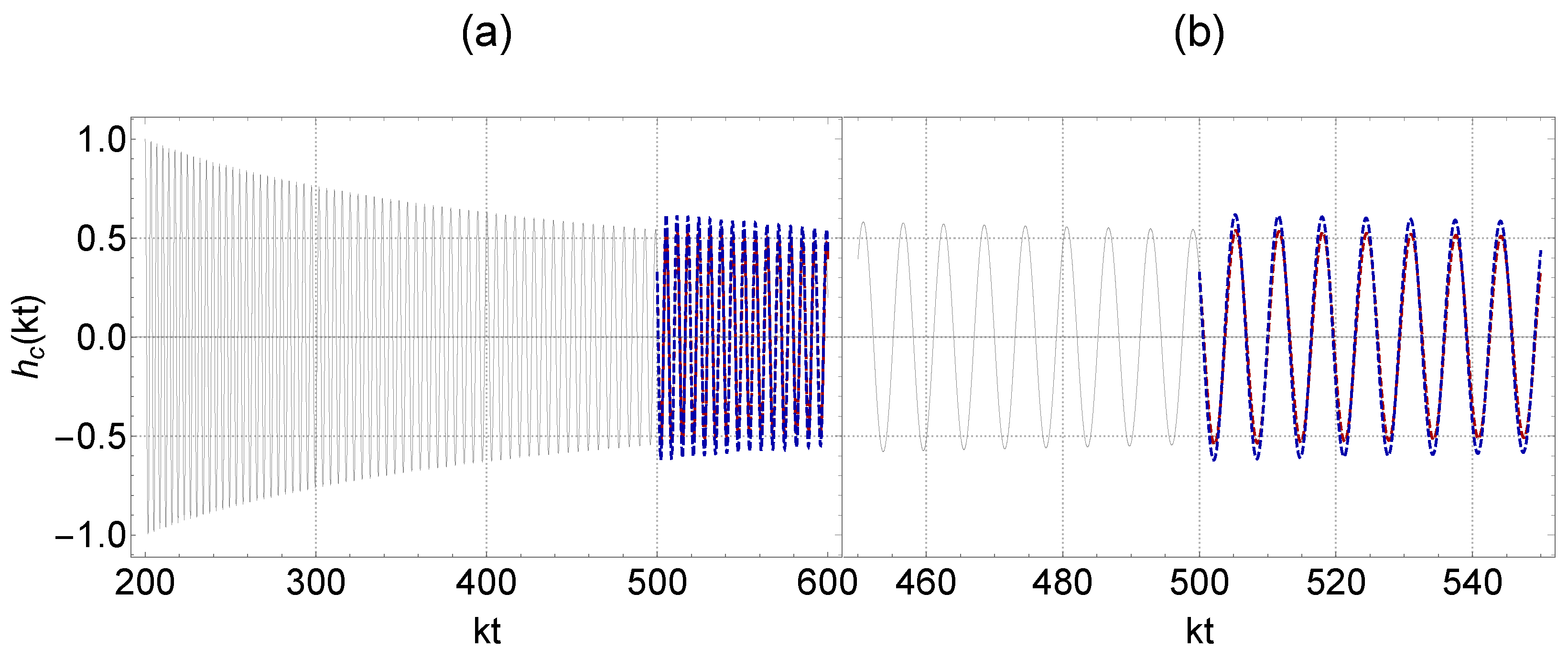
The waveform of the system exhibits a sudden change in behavior during the transition from the initial phase, which is represented by the gray waveform and occurs when the scale factor a is less than a s , to the final phase that occurs when a is greater than a s . At the value of the scale factor a s , a sudden cosmological singularity arises, leading to an abrupt shift in the system’s behavior.
Even though the factor β ˜ τ of the term h ˙ in differential equation (22) may be negligible at late times, any sudden change in β would result in observable effects at all anticipated scales.
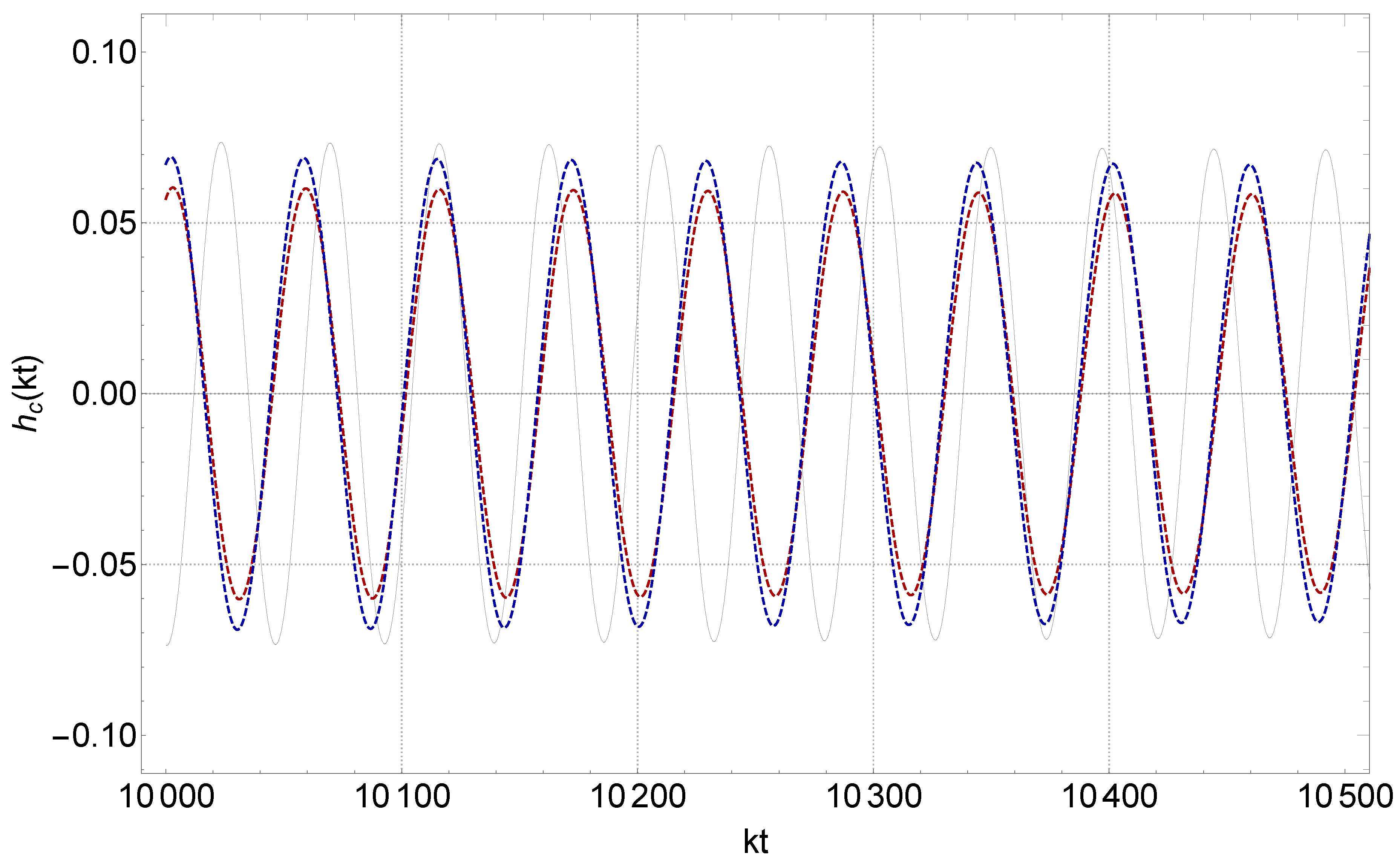
As a concrete eample we use initial conditions as h c ( τ = 200 ) = 1 and h c ( τ = 200 ) = 0 . Moreover, we assign specific values to the parameters, such as β = 2 3 , τ s = 500 , σ = 0.1 . We thus find the waveform evolution over the dimensionless rescaled time τ in both the context of General Relativity and the scalar tensor theory of gravitational transition frameworks. These are illustrated in Figure 1 and Figure 2.
The impulse induced by the Hubble flow through the friction term amplifies (or reduces) the amplitude at the moment of the transition (Figure 1) and results in a slightly faster (or slower decay) of the amplitude, compared to the initial phase depending on the sign of the Hubble rate discontinuity (Figure 2). In the given context, the value of σ , is positive, and there is an increase in damping, which arises from the interaction between the gravitational waves and the expanding universe. Therefore, if the damping becomes stronger (weaker), the amplitude of the gravitational wave strain would decay more (less) quickly. The third term in the dynamical equation for gravitational waves affects the wavelength of the oscillating waves. Thus a sudden increase of the expansion rate would lead to a larger scale factor at later times in the final phase and thus to a larger gravitational wave wavelength and period.
In summary, in the general relativistic transition scenario, the cosmological friction term and the third (driving) term in the gravitational wave equation act in different ways, where the former affects the rate of decay of the gravitational wave strain, while the latter affects the wavelength and period of the oscillations.
In the context of modified gravity, which involves modifying the propagation of gravitational waves by introducing an additional term α M [91,106] (illustrated in Figure 1 and Figure 2), the amplitude of the gravitational waves (blue waveforms) after the gravitational transition through scalar tensor theory of gravity, is altered compared to the red waveforms corresponding to transitions in the context of General Relativity. This amplitude may increase or decrease depending on the phase of the gravitational wave at the time of the transition and also on the sign of the δ -function impulse determined by the transition amplitude α .

3. Observational constraints on the transition amplitude from gravitational waves and other cosmological data

3.1. Monte Carlo data: Cosmological Parameters from the Einstein Telescope

The ET [75,76,81] is expected to significantly increase the number of detectable standard siren events due to its enhanced sensitivity and broader frequency range compared to current detectors like LIGO [84] and Virgo [85]. Although it is difficult to provide exact numbers, as the event rates depend on various factors such as the population of merging compact objects and their distribution in the universe, estimates suggest that the ET could detect thousands of standard sirens per year.
The ET’s increased sensitivity will allow it to observe gravitational wave events from much larger distances, reaching higher redshifts than current detectors[108,109,110,111,112,113]. While LIGO and Virgo can detect binary neutron star mergers up to a redshift of z 0.1 , the ET is expected to observe such events up to redshifts of z 2 or even higher [81,114]. This will enable the ET to probe the expansion history of the universe over a significant fraction of its age thus deriving constraints on cosmological parameters that are competitive with those obtained with electromagnetic waves.
It is important to note, however, that measuring the Hubble constant and other cosmological parameters using standard sirens not only requires detecting the gravitational wave signal but also identifying an electromagnetic counterpart to obtain the redshift[115,116]. This may be challenging for high-redshift events, as the associated electromagnetic signals could be fainter and harder to detect. Nevertheless, the significant increase in the number of standard siren events detected by the ET will provide a larger sample for Hubble constant measurements, even if only a fraction of the events have identifiable electromagnetic counterparts. A possible method to measure the redshift without associated electromagnetic signals is to use the statistical redshift estimation, which relies on galaxy catalogues and the probability of finding the source in each galaxy considering its mass and star formation rate[117,118,119].
The ET will measure cosmological parameters using gravitational waves (GW) from compact binary mergers, such as those involving neutron stars or black holes. One key aspect of this method is the determination of the GW luminosity distance.
The emitted GW waveform h c ( t ) resulting from the merger of two compact objects is reliant on various parameters, including the masses and spins of the merging objects, as well as the distance to the source and the inclination angle. Specifically, in the context of a gravitational wave originating from a compact binary coalescence, the amplitude of the strain in the gravitational wave can be expressed using the post-Newtonian (PN) approximation (the actual relationship can be more complex[120,121,122,123,124], especially when considering the full waveform of the gravitational wave signal), which incorporates PN corrections to the phase ϕ ( t ) but not to the amplitude and can be expressed as[96,97,107]:
h + ( t ) = 2 ( 1 + c o s 2 i ) d L ( z ) ( G N M c c 2 ) 5 3 ( π f ( t ) c ) 2 3 c o s [ ϕ ( t ) ]
h × ( t ) = 4 c o s i d L ( z ) ( G N M c c 2 ) 5 3 ( π f ( t ) c ) 2 3 s i n [ ϕ ( t ) ]
The redshifted chirp mass of a compact binary coalescence system is denoted as M c , and is related to the chirp mass M c through the expression M c = ( 1 + z ) M c . The chirp mass M c is a combination of the individual masses, m 1 and m 2 , of the binary system and is defined
M c = ( m 1 m 2 ) 3 5 ( m 1 + m 2 ) 1 5
The time-varying gravitational wave frequency f ( t ) evolves during the inspiral phase of the binary coalescence, and the inclination angle i is defined as the angle between the unit vector normal to the orbital plane and the line of sight[96,107]. By observing the gravitational waves and comparing the detected signal to theoretical templates, it is possible to extract these parameters, as well as the luminosity distance d L to the source. In particular, the amplitude of the gravitational waves decreases with the distance to the source. By comparing the calculated intrinsic amplitude (which depends on the chirp mass) with the observed amplitude (which depends on the distance), the luminosity distance to the source can be estimated.
The luminosity distance d L can be expressed in terms of the scale factor a ( t ) , the Hubble parameter H ( z ) , and the redshift z in a flat universe as:
d L ( z ) = ( 1 + z ) 0 z c H ( z ) d z
where c is the speed of light, and H ( z ) is the Hubble parameter as a function of redshift z. The Hubble parameter for a flat universe is parameterized by the density parameter Ω m , 0 , for matter, as
H 2 ( z ) = H 0 2 Ω m , 0 ( 1 + z ) 3 + 1 Ω m , 0
Here, H 0 is the Hubble constant, and z is the redshift. By combining the expressions for d L ( z ) and H ( z ) , we can relate the luminosity distance to cosmological parameters:
d L ( z ) = ( 1 + z ) 0 z c H 0 Ω m , 0 ( 1 + z ) 3 + 1 Ω m , 0 d z
By measuring the luminosity distance d L from gravitational wave events and obtaining the redshift z (eg from the electromagnetic counterpart), we can fit this expression to a sample of standard siren events to estimate the cosmological parameters, such as the Hubble constant H 0 , the matter density parameter Ω m , 0 , and the dark energy density parameter Ω Λ .
In order to estimate the anticipated constraints to be imposed on cosmological parameters from luminosity distance measurements of the ET we construct a mock dataset of 1000 standard sirens that could be obtained by GW observations of the ET [80] assuming an underlying Planck18/ Λ CDM model. We thus derive Monte-Carlo measurements of d L ( z i ) of binary systems and the corresponding redshifts z i of each binary system. Then we use these data to fit the Hubble flow H ( z ) assuming an underlying Λ C D M model or a sudden leap model which has two additional parameters (the transition amplitude and the transition redshift).
Following [80], we generate a catalogue of 1000 events in the redshift range z [ 0.07 , 2 ] . The interval has a z m a x = 2 which leads to an angle-averaged signal-to-noise ratio above 8 [77,80]. There is a minimum redshift cut off, depending on the sensitivity of the detector (ET), which is taken as z m i n = 0.07 [80], in order to exclude galaxies with peculiar velocities comparable with their recessional velocities due to the Hubble flow.
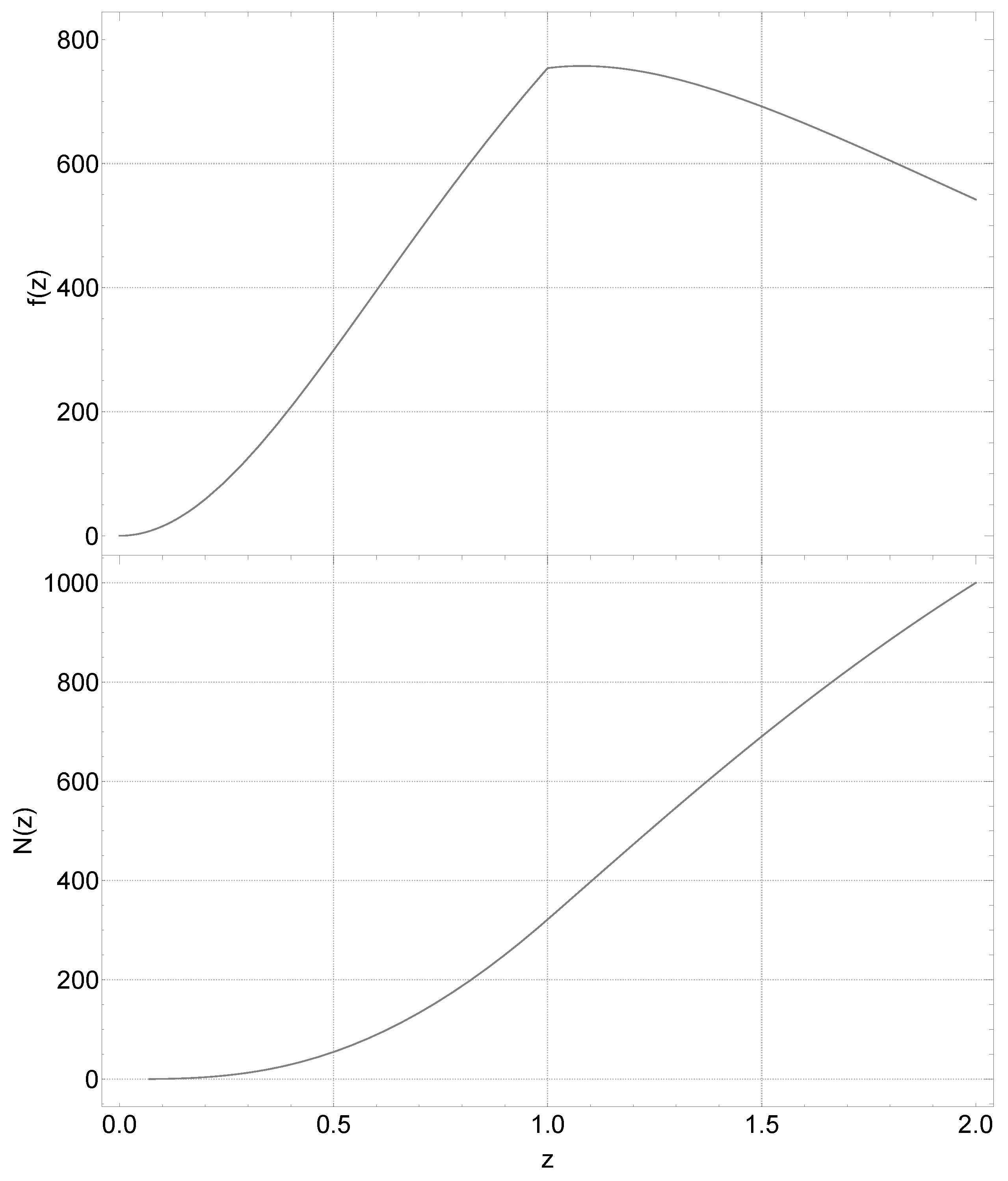
The probability for finding a standard siren with the ET in the redshift range [ z , z + d z ] is given by the number density function [77,80]:
f ( z ) d z = N 0 4 π r c o a l ( z ) d L 2 ( z ) H ( z ) ( 1 + z ) 3 d z
where r c o a l ( z ) is the coalescence rate at redshift z [77]:
r c o a l ( z ) = 1 + 2 z i f z 1 15 3 z 4 i f 1 < z < 5 0 i f z 5
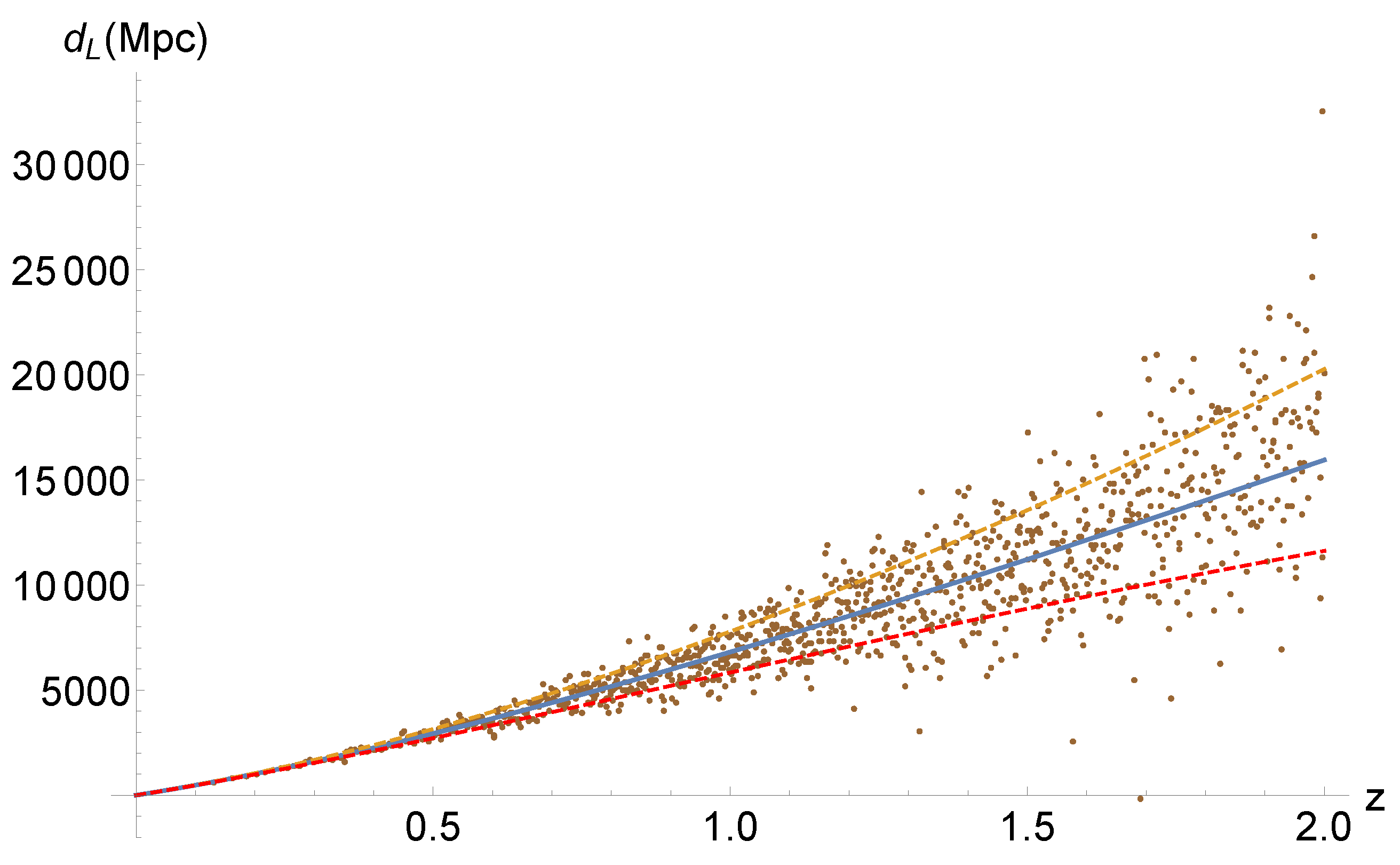
The normalization constant of eq. (43) N 0 is determined by requiring that the integral N 0 0.07 2 4 π r ( z ) d L 2 ( z ) H ( z ) ( 1 + z i ) 3 d z = 1000 . Using (43) we thus construct the "cumulative distribution" function N ( z ) (see Figure 3) of the 1000 standard sirens through the integral N ( z ) = 0.07 z f ( z ) d z , in order to generate the redshifts z = z i . Our approach involves the use of the Newton-Raphson method to solve a set of 1000 equations, of the form N ( z i ) = i for i 1 , 2 , , 1000 . The objective is to obtain the corresponding redshift z i , which lies in the interval [ 0.07 , 2 ] , for each equation solved.
In that manner, the redshifts are distributed through the interval [ 0.07 , 2 ] with respect to the number density function (43). In accordance with the discussion presented in [80], a set of 1000 sources is generated. The luminosity distance of each source at redshift z i is obtained by randomly varying normally distributed luminosity distances around a mean value d ¯ L ( z i ) . The value of d ¯ L ( z i ) is predicted by the hypothesized Planck18/ Λ CDM model with Ω m , 0 = 0.3166 and H 0 = 67.27 k m s M p c 1 [1]. The resulting luminosity distance is calculated as follows
d ¯ L ( z i ) = c ( 1 + z i ) H 0 0 z i d z 1 Ω m , 0 + Ω m , 0 ( 1 + z ) 3
We assume that the luminosity distance d L ( z i ) of each source, is normal distributed across an interval of the mean luminosity distance, centered at d ¯ L ( z i ) with standard deviation [80,125,126]
σ i Δ d L ( z i ) d ¯ L ( z i ) ( 0.1449 z i 0.0118 z i 2 + 0.0012 z i 3 ) 2 + ( 0.05 z i ) 2
where the term 0.05 z i is uncertainty induced by weak lensing [126] and the term 0.1449 z i 0.0118 z i 2 + 0.0012 z i 3 is uncertainty due to instrumental error calculated modeled by Monte Carlo simulations (see [77]). The Gaussian probability density function (PDF), with a standard deviation given by the relation (46), is written as
P D F ( X i ) = 1 σ i 2 π e 1 2 ( X i d ¯ L ( z i ) σ i ) 2
where X i corresponds to the randomly generated luminosity distance of a standard siren i. Figure 4 provides a visual representation of a realization of the resulting data luminosity distance.
Using these data generated under the assumption of an underlying Planck18/ Λ CDM model we can test the type of constraints that would be imposed on a cosmological model involving a discontinuity of H ( z ) due to a transition of the gravitational constant G eff ( z ) . The predicted luminosity distance for this class of models is:
d L ( z ; Ω m , 0 , h , α , z s ) = ( 1 + z ) 0 z c d z H 0 [ 1 + α Θ ( z z s ) ] 1 2 1 Ω m , 0 + Ω m , 0 ( 1 + z ) 3
where the Hubble constant is H 0 = 100 h k m s M p c . In the context of a modified theory of gravity, the hypothesized transition of the gravitational constant would be associated with a mismatch between the luminosity distance d L em of the light travels and the gravitational wave luminosity distance d L gw [80].
In the context of an evolving G eff the measured d L gw ( z ) by standard sirens [80,97,107,127] would lead to a luminosity distance of the form [80] shown in eq. (10).
Thus the luminosity distance measured by gravitational waves may be written as
d L gw ( z ; Ω m , 0 , h , α , z s ) = [ 1 + α Θ ( z z s ) ] 1 2 ( 1 + z ) 1 0 z c d z H 0 [ 1 + α Θ ( z z s ) ] 1 2 1 Ω m , 0 + Ω m , 0 ( 1 + z ) 3
and the cosmological parameters of a cosmological model involving a gravitational transition with amplitude α occuring at redshift z s may be constrained by minimizing χ 2 defined as
χ sirens 2 = i = 1 1000 [ d L gw ( z i ; Ω m , 0 , h , α , z s ) d ¯ L ( z i ) ] 2 σ i 2
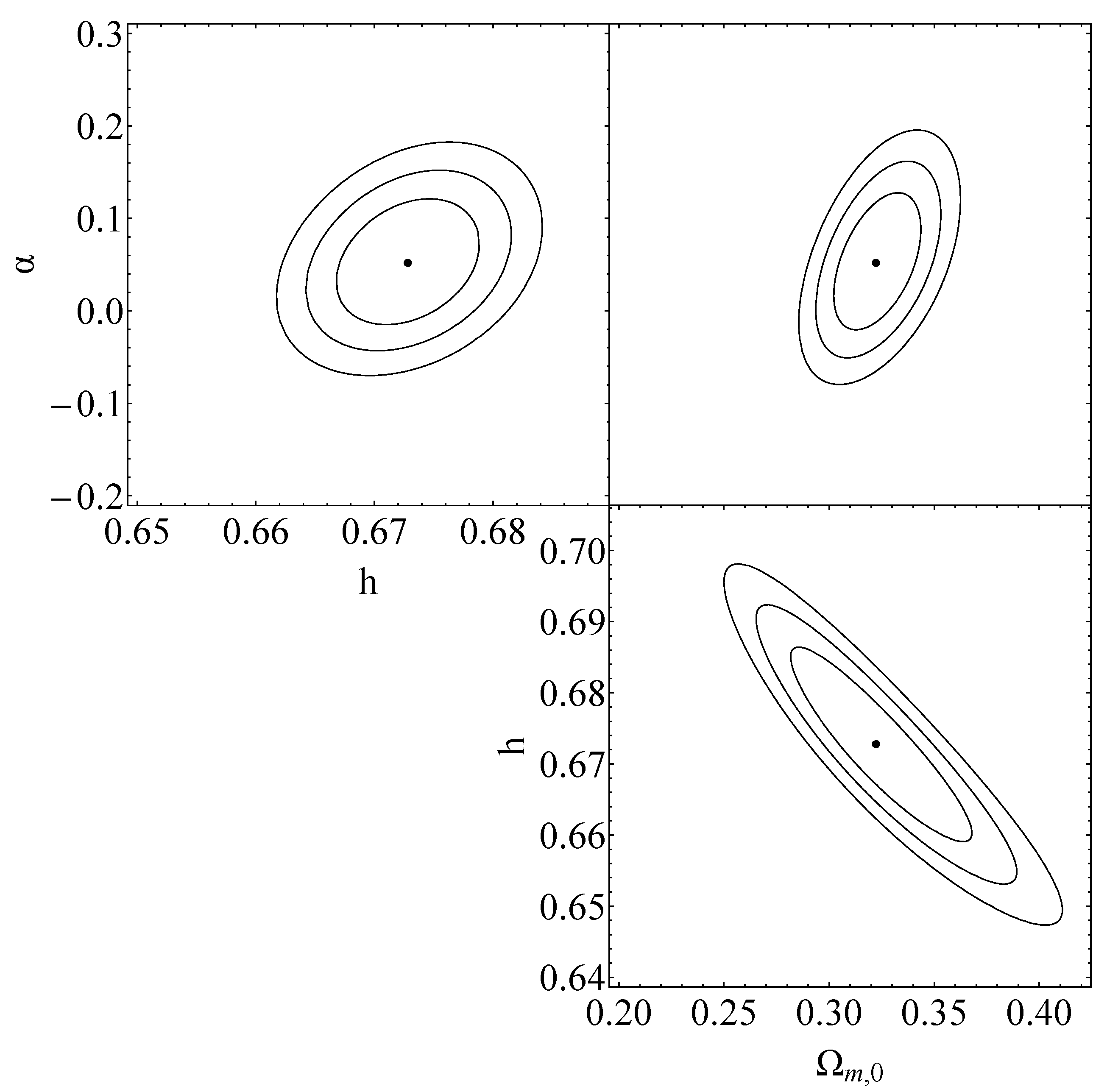
Since the assumed underlying model is Planck18/ Λ CDM and involves no transition, this fit to the Monte-Carlo data is useful only in predicting the level of uncertainties in the anticipated constraints on the sudden leap model parameters anticipated from the ET data. These predicted constraints are shown in Figure 5 and are clearly consistent with α = 0 since the assumed underlying model is Planck18/ Λ CDM 2.

3.2. Real data: BAO+CMB

In the early universe prior to recombination, initial perturbations evolved into overdensities through gravitational interactions with dark matter. Baryonic matter was embedded within these dark matter overdensities and the collapse of these overdensities was followed by radiation-induced overpressure. This overpressure, in turn, generated an expanding sound wave that propagated through plasma at a velocity of
c s = c 3 ( 1 + R s )
Here, R s 3 ρ b 4 ρ γ , where ρ b represents the baryon density and ρ γ represents the photon density. The fluid undergoes damped oscillations in both space and time, wherein the oscillation period depends on the sound speed. The sound speed c s is depending on the density of baryonic matter. When the density of baryons is considerably lower than that of radiation, the sound speed assumes the typical value for a relativistic fluid, i.e. c s = c / 3 . However, the introduction of baryonic matter increases the mass of the fluid, leading to a decrease in the sound speed.
If we denote as r s ( z ) the sound horizon, i.e. the comoving distance traveled by a sound wave from the Big Bang till a corresponding redshift z, then [53,102]
r s ( z ) = 1 H 0 z d z c s ( z ) E ( z )
The sound horizon r s ( z drag ) marks the distance over which sound waves propagated. The redshift z drag denotes the period of the drag epoch i.e. the epoch when the baryons were released from the Compton drag of photons, which occurred slightly after recombination in the early universe. Eisenstein et al.[128] obtained a suitable fitting formula for the redshift z drag as
z drag = 1291 ( Ω m , 0 h 2 ) 0.251 1 + 0.659 ( Ω m , 0 h 2 ) 0.828 [ 1 + b 1 ( Ω m , 0 h 2 ) b 2 ]
where the parameter b 1 is
b 1 = 0.313 ( Ω m , 0 h 2 ) 0.419 [ 1 + 0.607 ( Ω m , 0 h 2 ) 0.674 ]
and b 2 as
b 2 = 0.238 ( Ω m , 0 h 2 ) 0.223
The Baryon Acoustic Oscillation (BAO) measurements, which detect the presence of a characteristic scale in the matter distribution, offer a standard ruler that is valuable for deducing the expansion history of the universe and estimating other cosmological parameters. These measurements provide constraints on several quantities, specifically [129]:
d M × r s fid r s , d V × r s fid r s , d H × r s fid r s
In the above equations, r s fid represents the sound horizon in the fiducial cosmology. The Hubble distance, denoted by d H , is a characteristic length scale of the universe and can be expressed as:
d H ( z ) = c H 1 ( z )
We define the angular diameter distance, d A , and proper motion distance, d M . These distances are related as follows:
d M ( z ) = ( 1 + z ) d A ( z ) = d L ( z ) 1 + z
The related effective distance, d V ( z ) [130], is given by the equation:
d V ( z ) = [ c z d M 2 ( z ) H ( z ) ] 1 3
In terms of measurements, there are two possible directions: the line-of-sight dimension and the transverse direction. These measurements involve the ratios δ z s r s ( z ) H ( z ) c and θ s ( z ) r s ( z ) d M ( z ) . The spherically averaged spectrum is connected to the effective distance, which can be expressed as:
[ θ s 2 ( z ) δ z s ] 1 3 = z 1 3 r s ( z ) d V ( z )
A fitting formula, developed by Hu & Sugiyama, 1995 [131], can be utilized to derive the redshift z associated with the photon decoupling surface. For values of the baryon density parameter Ω b in the range 0.0025 Ω b 0.25 and the matter density parameter Ω m , 0 in the range 0.025 Ω m , 0 0.64 , z can be expressed as:
z = 1048 [ 1 + 0.00124 ( Ω b h 2 ) 0.738 ] [ 1 + g 1 ( Ω m , 0 h 2 ) g 2 ]
g 1 = 0.0783 ( Ω b h 2 ) 0.238 1 + 39.5 ( Ω b h 2 ) 0.763 , g 2 = 0.560 1 + 21.1 ( Ω b h 2 ) 1.81
The baryonic acoustic oscillation (BAO) leaves a characteristic imprint on the power spectrum of the cosmic microwave background (CMB) anisotropies, which is observed as a series of peaks and troughs. The characteristic angle, θ A , which defines the location of the peaks can be calculated by the following equation[53]:
θ A = r s ( z ) d M ( z )
The angular power spectrum of the CMB is decomposed into its multipole moments, where the low multipole moments correspond to the large angular scales and the high multipole moments correspond to the small angular scales. Each multipole l that corresponds to the characteristic angle θ A can be determined by the following equation [53]:
l A = π θ A = π d M ( z ) r s ( z )
The shift parameter, denoted as R, is a dimensionless parameter that provides a rescaled representation of the ratio between the proper transverse velocity and the observed angular velocity of an object at the photon decoupling surface. It encompasses information related to the comparison of predicted and observed positions of the acoustic peaks in the cosmic microwave background (CMB). Its formal definition is as follows [53]:
R Ω m , 0 H 0 2 d M ( z ) c
To impose constraints on cosmological parameters, we have followed the work of [129,132,133]. Throughout the next sections, we incorporate the induced transition in the Hubble flow, which is
H ( z ; Ω m , 0 , h , α , z s ) = H 0 [ 1 + α Θ ( z z s ) ] 1 2 1 Ω m , 0 + Ω m , 0 ( 1 + z ) 3

3.2.1. CMB measurements

The analysis incorporates Planck data, consisting of temperature and polarization data, along with CMB lensing. Zhai et al. [133] provide the CMB data, which is represented by a data vector and a covariance matrix. The data vector associated with it is expressed as follows
v = 1.74963 301.80845 0.02237
and also the covariance matrix is written[133]:
[ C C M B ] = 10 8 × 1598.9554 17112.007 36.311179 17112.007 811208.45 494.79813 36.311179 494.79813 2.1242182
The χ CMB 2 distribution as [133]:
χ CMB 2 = v T [ C C M B ] 1 v
where in a flat universe the vector is written as[133]
v = R 1.74963 l A 301.80845 Ω b h 2 0.02237
By adopting the luminosity distance (48) and the proper motion distnce, as defined in (58), then
l A = π d M ( z ; Ω m , 0 , h , α , z s ) r s ( z ; Ω m , 0 , h , α , z s )
and the shift parameter is
R Ω m , 0 H 0 2 d M ( z ; Ω m , 0 , h , α , z s ) c

3.2.2. BAO measurements

The distribution of matter exhibits distinct patterns known as baryonic acoustic oscillations (BAO), which are reflected in the spatial distribution of galaxies. Numerous astronomical surveys, such as the 6-degree Field Galaxy Survey (6dFGS), the WiggleZ surveys, the Sloan Digital Sky Survey (SDSS), and the Lyman-alpha (Ly- α ) survey, have been conducted to map out the distribution of galaxies.
To quantify the BAO measurements, the χ BAO 2 distribution is computed following the methodology outlined in [132,134]. The expression for χ BAO 2 is given as:
χ BAO 2 = χ 6 d F G s , W i g g l e 2 + χ S D S S 2 + χ L y a 2
The surveys 6dFGs[135] and WiggleZ [136] constitute the following distribution
χ 6 d F G s , W i g g l e 2 = v i ( [ C 6 d F G s , W i g g l e ] 1 ) i j v j
Those surveys give a measurement for the ratio
d z ( z ) r s ( z drag ) d V ( z )
which constitutes the components
v i = d z ( z i ; Ω m , 0 , h , α , z s ) | t h e o r y d z ( z i ) | o b s e r v e d
where the d z ( z i ; Ω m , 0 , h , α , z s ) is defined through the equations (48),(58). The corresponding data vectors are[132]
z d z σ = 0.106 0.336 0.015 , 0.44 0.073 0.031 , 0.6 0.0726 0.0164 , 0.73 0.0592 0.0185
and also the total covariance matrix [132]:
[ C 6 d F G s , W i g g l e ] 1 = 1 0 . 015 2 0 0 0 0 1040.3 807.5 336.8 0 807.5 3720.3 1551.9 0 336.8 1551.9 2914.9
To analyze the SDSS data by constraining d V × r s fid ( z drag ) r s ( z drag ) we utilize the data vectors provided in [132] and if the value r s fid ( z drag ) = 149.28 M p c , then
z 1 d z σ = 0.15 4.465666824 0.1681350461 , 0.32 8.4673 0.167 , 0.57 13.7728 0.134
the corresponding distribution for SDSS data is [132]
χ S D S S 2 = i = 1 3 [ 1 d z ( z i ; Ω m , 0 , h , α , z s ) | t h e o r y d V ( z i ) r s ( z drag ) | o b s e r v e d ] 2 σ i 2
The Ly- α survey constrains d H r s and d M r s respectively (see also [132]). While the corresponding data vectors are [132]
v 1 = z d M ( 1 + z ) r s ( z drag ) σ 1 + z = 2.34 11.20 0.56 , v 2 = z d H r s ( z drag ) σ = 2.34 8.86 0.29
which they constitute the covariance matrix
[ C L y α ] 1 = 1 0 . 56 2 0 0 1 0 . 29 2
The distribution for Ly- α data χ L y a 2 = v T [ C L y α ] 1 v is constituted by the covariance matrix (80) and the folllowing vector[132]
v = d A ( z i ) r s ( z drag ) | o b s e r v e d d A ( z i ; Ω m , 0 , h , α , z s ) r s ( z drag ; Ω m , 0 , h , α , z s ) | t h e o r y d H ( z i ) r s ( z drag ) | o b s e r v e d d H ( z i ; Ω m , 0 , h , α , z s ) r s ( z drag ; Ω m , 0 , h , α , z s ) | t h e o r y
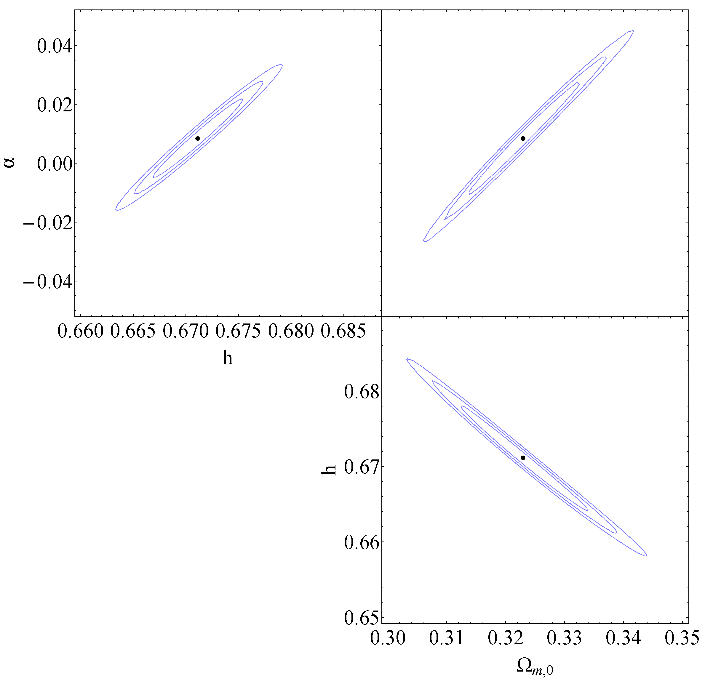
The resulting contours3 are shown in Figure 6.

3.3. Real data: Pantheon+

Type Ia supernovae, characterized by the absence of a spectral line of hydrogen and the presence of an absorption line attributed to singly ionized silicon, result from the explosion of a white dwarf in a binary system that surpasses the Chandrasekhar limit due to gas accretion from a companion star.
Importantly, Type Ia supernovae exhibit a nearly constant absolute luminosity at the peak of their brightness, denoted by an established absolute magnitude of approximately M 19 . As a result, the distance to a Type Ia supernova can be deduced through the observation of its apparent luminosity. By concurrently measuring the apparent magnitude and the light curve, it becomes feasible to predict the corresponding absolute magnitude [53].
Brighter supernovae exhibit broader light curves (flux or luminosity of the supernova as a function of time). It is important to note that when referring to the universal absolute magnitude of Type Ia supernovae hereafter, it is implied that the magnitude has been appropriately adjusted to account for the light curve width.
When considering the luminosity distance d L measured in megaparsecs (Mpc), the concepts of absolute magnitude, apparent magnitude, and luminosity distance can be formally related as follows [53]:
μ m M = 5 log 10 d L Mpc + 25
Here, μ represents the distance modulus, which quantifies the difference between the apparent magnitude m and the absolute magnitude M of an object.
In the context of modified gravity, an abrupt transition in G eff results in a luminosity distance as predicted by (48). In the event that the luminosity peak is proportional to the absolute magnitude M[137](see Equation (82)), a sudden increase in the effective gravitational constant G eff would result in a supernova exhibiting diminished brightness relative to the predictions derived from conventional scenarios[40].
The Pantheon+ data set comprises a collection of 1550 Type Ia supernovae and 1701 corresponding light curves, spanning a redshift range of 0.001 < z < 2.26 [138]. To analyze the Pantheon+ data, we adopt the methodology outlined in the works of Brout et al. (2022) [138].
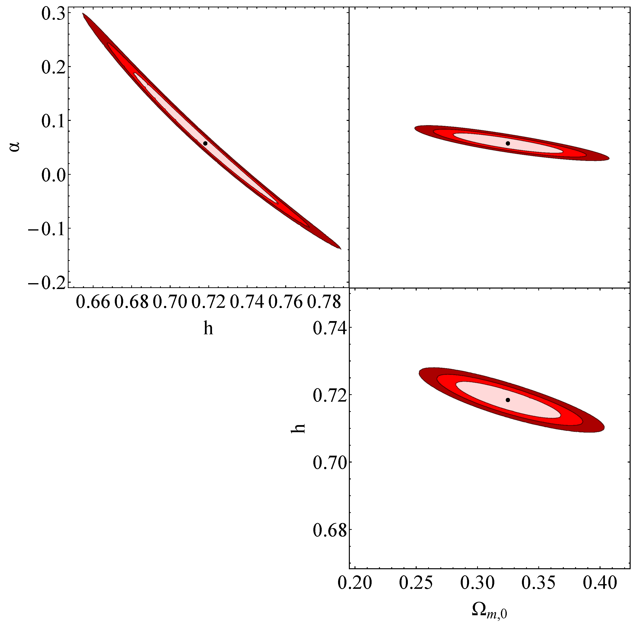
Figure 7. The red contours in the h α , Ω m , 0 h , and Ω m , 0 h diagrams represent the projected 1 3 σ confidence regions obtained from analyzing the Pantheon+ data within the sudden leap model (sLCDM). The best fit values for the transition occurring at a s = 0.995 ± 0.004 and M = 19.24 ± 0.03 , along with the corresponding best fit values of Ω m , 0 , h, and α , can be found in Table 2.
Preprints 76318 g007
If we denote the 1701 × 1701 covariance matrix as [ C s t a t + s y s t ] which is provided with Pantheon+ data including both statistical and systematic uncertainties and if we begin with the minimization a χ 2 distribution
χ 2 = Q T [ C s t a t + s y s t ] 1 Q
then due to degeneracy, it becomes impossible to estimate H 0 as there is a correlation between H 0 and the absolute magnitude of SnIa, denoted as M.
The vector Q represent a quantity with 1701 components and each one is defined as
Q i = m B i M μ m o d e l ( z i ; Ω m , 0 , h , α , z s )
The predicted distance modulus is denoted as μ m o d e l , which is obtained using the assumed sudden leap model. If the luminosity distance d L is given in (48), then
μ m o d e l ( z i ; Ω m , 0 , h , α , z s ) = 5 log 10 ( d L ( z i ; Ω m , 0 , h , α , z s ) M p c ) + 25
The estimate of H 0 was not possible in the first Pantheon sample [139] because of the degeneracy between H 0 and SnIa absolute magnitude M.
To resolve the degeneracy issue in the Pantheon+ dataset, a modification was made to the vector Q by incorporating the distance moduli of SnIa in Cepheid hosts μ C e p h , which can constrain M independently. Thus the modified vector Q is [138]
Q i = m B i M μ C e p h ( z i ) i f i C e i p h e i d h o s t s m B i M μ m o d e l ( z i ; Ω m , 0 , h , α , z s ) o t h e r w i s e
which μ C e p h ( z i ) is the corrected distance modulus of the Cepheid host of the i t h SnIa which is measured independently in the context of the SH0ES distance ladder with Cepheid calibrators[10]. Thus, the degeneracy between M and H 0 is shattered and the parameters M , H 0 , Ω m , 0 , α , z s can be estimated by implementation of the
χ P a n t 2 = Q T [ C s t a t + s y s t ] 1 Q
The resulting contours4 are shown in Figure 8.

3.4. Combined Data

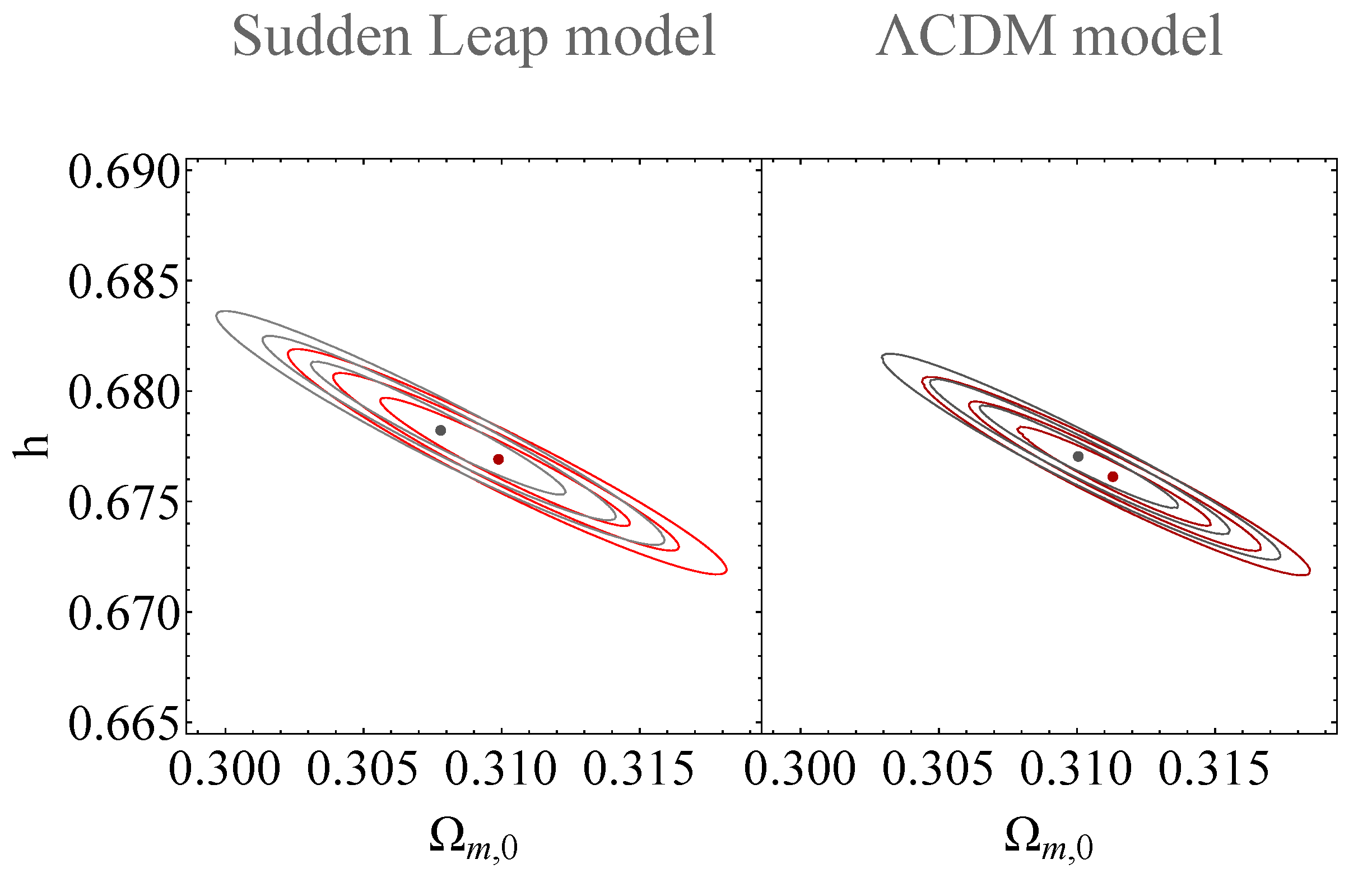
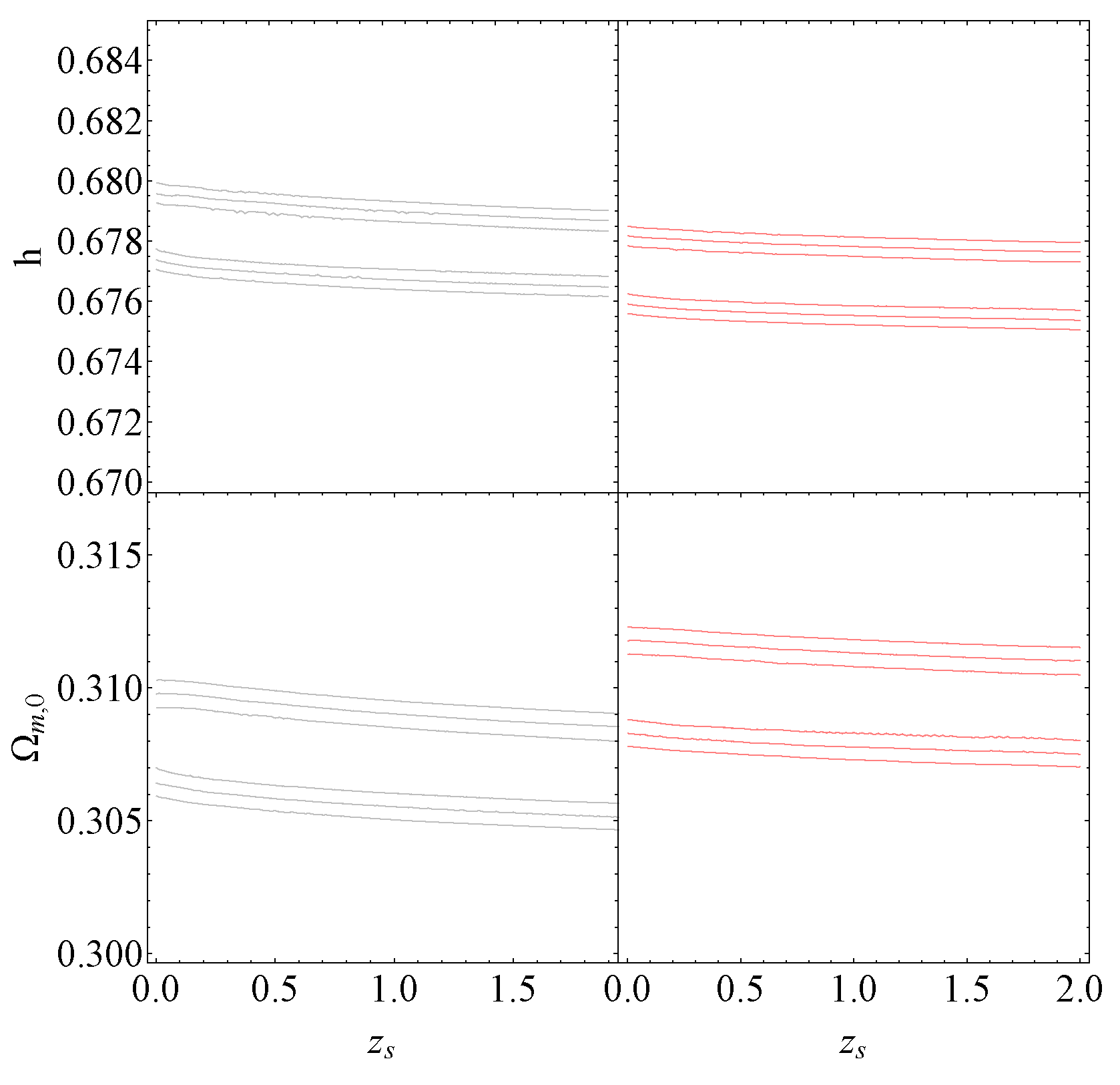
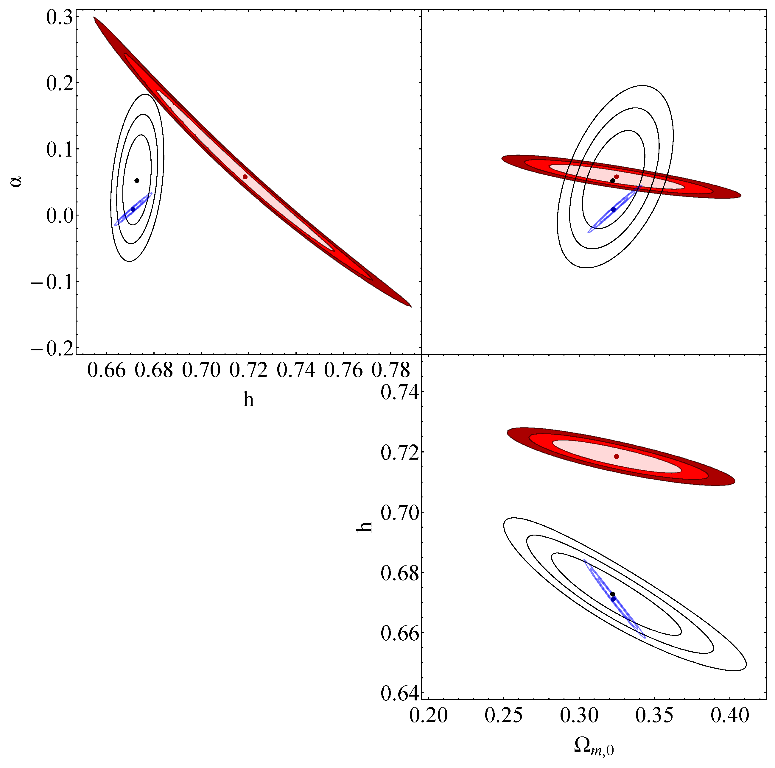
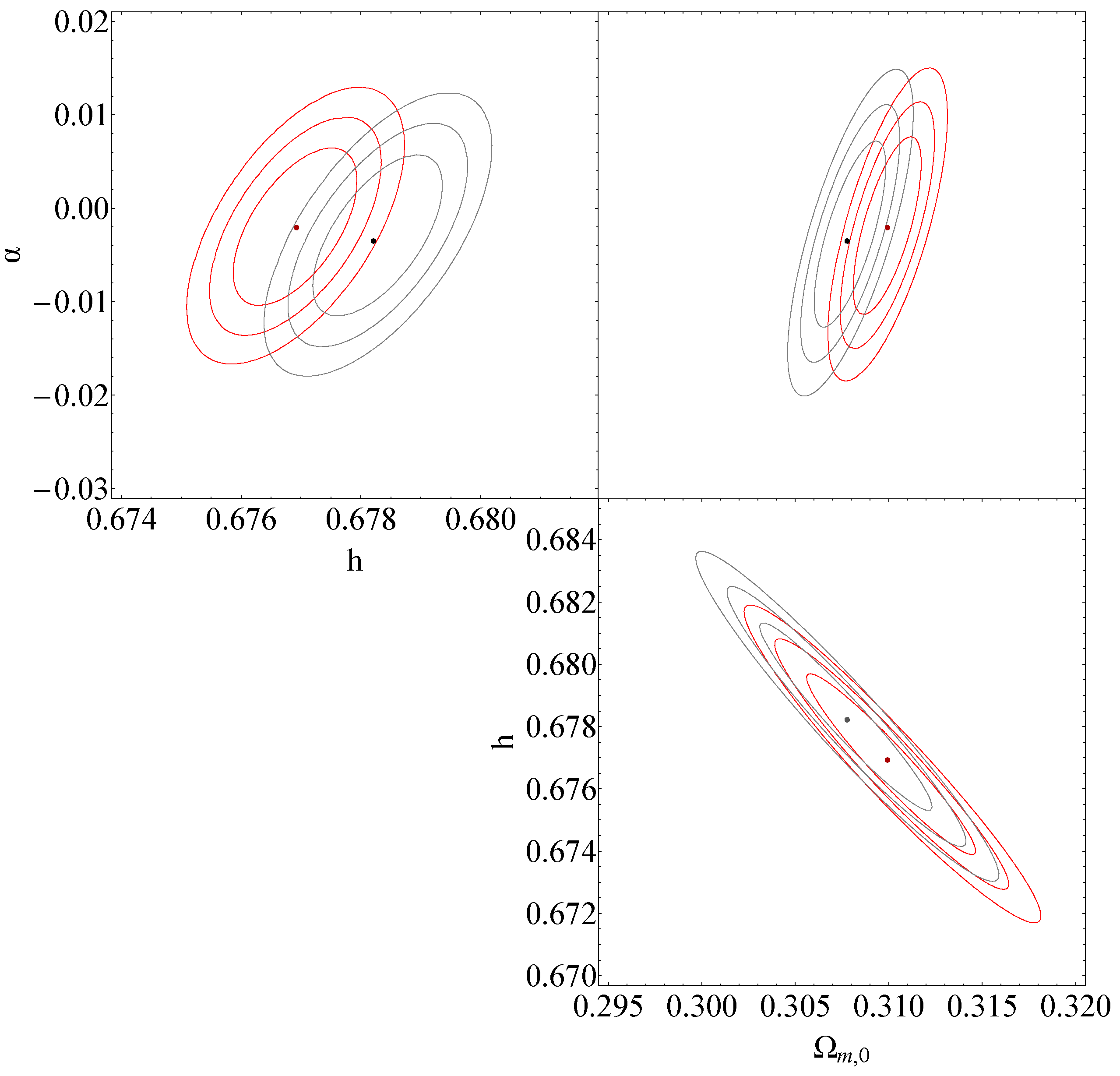
By minimizing the χ 2 and considering a range defined as χ min 2 ± Δ χ n σ 2 (as described in Appendix B), we can determine the projected confidence regions for each pair of parameters by fixing the parameters that are not directly studied to their best fit values. The confidence levels of 1 σ , 2 σ , and 3 σ are indicated by the red and gray contours in Figure 9.
When combining the CMB, BAO, Standard Sirens, and Pantheon+ data, the corresponding χ 2 distribution is obtained by summing the individual χ 2 contributions:
χ 2 = χ sirens 2 + χ BAO 2 + χ Panth 2 + χ CMB 2
Specifically, we set the values of a s = 0.812 ± 0.2 and M = 19.43 ± 0.015 , and additionally fix Ω m , 0 = 0.31 ± 0.005 or h = 0.677 ± 0.003 or α = 0.001 ± 0.005 for each diagram, respectively. This approach is consistent across all three diagrams. For example, in the h α diagram, the fixed best fit values are Ω m , 0 = 0.31 ± 0.005 , a s = 0.812 ± 0.2 , and the absolute magnitude M = 19.43 ± 0.015 .
The Table 2 provides the details of the best fit values. To construct the h α , Ω m , 0 α , and Ω m , 0 h diagrams presented in Figure 9, certain parameters are fixed. The Figure 9 illustrates the contours in gray, representing the χ 2 distribution as defined in equation (89). These contours correspond to the combined contributions from χ BAO 2 , χ Panth 2 , and χ CMB 2 given by:
χ 2 = χ BAO 2 + χ Panth 2 + χ CMB 2
The resulting contours5 are shown in Figure 9.

3.5. Results

The generated mock data are obtained by assuming the Planck18 values (Planck Collaboration, 2018 [1]), which explains the close proximity of the best fit values for Ω m , 0 and H 0 derived from both standard sirens and the combination of CMB+BAO data (Figure 8). The case where the value of the transition amplitude is α 0 , appears to be disfavored by the data, as the value α = 0 consistently falls within the 1 σ range in all cases. It is important to highlight that the analysis of the Pantheon+ data suggests a potential quasi-degeneracy between the Hubble constant dimensionless parameter h, and the transition amplitude α . Furthermore, the Pantheon+ dataset indicates that the best fit value for the scale factor is a s = 0.995 ± 0.004 ( z s = 0.005 ), and the corresponding luminosity distance at z s is approximately d L ( z s ) 20.96 Mpc, as determined by Equation (48). Notably, this luminosity distance value is close to the estimate of a sudden change in the intrinsic luminosity distance of SnIa by [40,41,44,140], which predicts a value of approximately 20 Mpc.
The present theoretical framework of the sudden leap model is characterized by the formation of a true vacuum bubble. This phenomenon arises from a phenomenological first-order phase transition of a scalar field, exemplified by Equation (7). The transition extends over an approximate luminosity distance of 20.96 Mpc. Within the confines of this true vacuum bubble, there is a transition in the effective gravitational constant, represented by G eff . Consequently, the encounter of bound systems [52] or gravitational waves with the boundary of this vacuum bubble gives rise to profound physical effects akin to those associated with a sudden cosmological singularity.
The assessment of accuracy in parameter estimation entails the evaluation of the ratio between the projected one-dimensional likelihoods and their corresponding best fit values. This ratio acts as a quantification of the constraining power demonstrated by a particular set of measurements, centered on their respective best fit values.
The inclusion of the Pantheon+ data alongside the CMB, BAO data appears to result in a degradation of the predicted accuracy at the best fit value of h and Ω m , 0 for the sudden leap model. This can be attributed to a plausible quasi-degeneracy between the parameters h and α . Conversely, the addition of standard sirens into the parameter estimation process results in an enhancement of the accuracy for the sudden leap model, in all cases considered (see Table 3).
To identify the best model for future observations, we can use the Akaike Information Criterion (AIC). Given a set of models, the AIC helps us select the model that best describes the data. The criterion estimates the expected, relative information loss between the fitted model and the observed data. The AIC factor is expressed as [141]:
A I C = 2 k 2 ln ( L ^ )
The likelihood function could be defined L e 1 2 χ 2 and has a maximum value L ^ e 1 2 χ m i n 2 , and the term k represents the number of the parameters in the model (see [141]). When comparing a set of models, it is not the absolute value of the AIC that is important, but rather the difference between the AIC values of the corresponding pair of models. In the case of a set of models that includes both the Λ CDM model and the sudden leap model, we use the AIC differences, or Δ i = A I C s L C D M A I C Λ C D M , to assess the empirical support for each model [141,142].
A Δ i value between 0 and 2 indicates substantial empirical support for the i-model, while a value between 4 and 7 suggests considerably less support. If Δ i exceeds 10, the empirical support for the i-model is essentially none. We can compare the hypothesized model with the Λ CDM model.
To evaluate the relative probability of the i-model occurring, we set e 1 2 Δ m i n 1 for the estimated best model, and use the ratio e 1 2 Δ i [141].
For example, the sudden leap model is about 0.264 times as probable as the Λ CDM model in minimizing the information loss of Pantheon+ data. The current datasets does not seem to favor the sudden leap model over the Λ CDM model in any case.
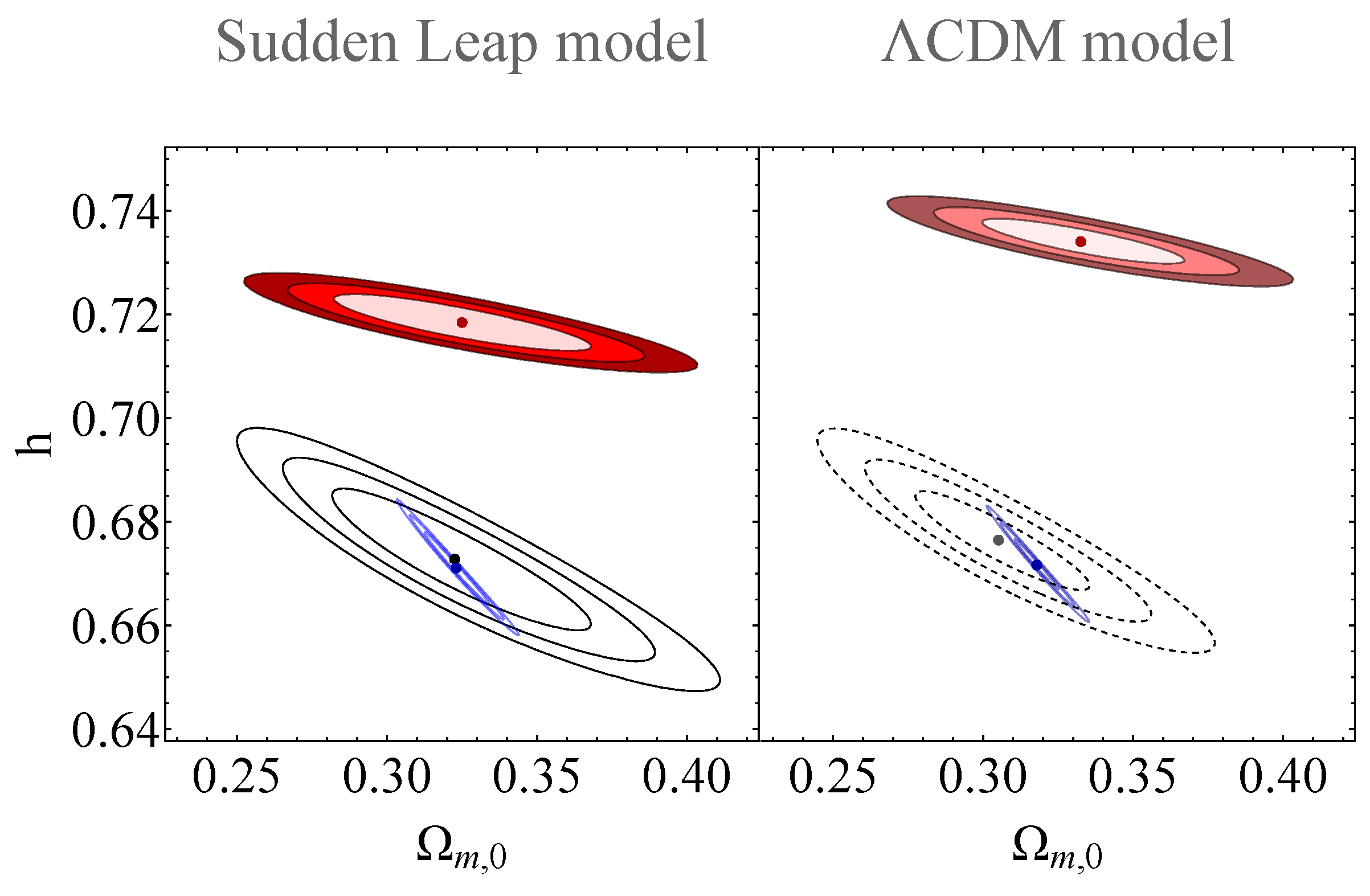
Figure 11. The resulting contours which correspond to the confidence regions sketched around the minimum of χ P a n t 2 + χ BAO 2 + χ CMB 2 (gray) and χ P a n t 2 + χ BAO 2 + χ CMB 2 + χ sirens 2 (red) of the sudden leap model in contrast to the corresponding confidence regions sketched around the minimum of χ P a n t 2 + χ BAO 2 + χ CMB 2 (gray hue) and χ P a n t 2 + χ BAO 2 + χ CMB 2 + χ sirens 2 (red hue) of the Λ CDM model(see Appendix C).
Preprints 76318 g011
Standard sirens χ sirens 2 , when they added to the data, with χ P a n t 2 + χ BAO 2 + χ CMB 2 , improve the accuracy at the parameter estimation. This improvement would have been larger if the consistency between Standard Sirens and Pantheon+ data was higher. Notice that for the generation of the sirens mock data we have assumed Planck18/ Λ CDM model parameters which are not fully consistent with the Pantheon+ best fit Λ CDM parameter values. This tension tends to increase the uncertainty of the best fit parameter values when these datasets are combined.
Even though the increase in constraint level is relatively small (Figure 9), standard sirens have systematic errors completely independent from the rest of the data [80]. For these reasons, standard sirens going to have a key role at the parameter constraining on the future.

4. Conclusion-discussion

It has been suggested that the Hubble tension i.e. the disparity in the Hubble constant measurements at low and high redshifts, could potentially be accounted for by an abrupt transition in the effective gravitational constant taking place within a range of redshifts less than z s < 0.01 [38]. Herein, we explored the consequences of such a hypothesis by considering an underlying scalar tensor theory gravity and identifying the effects of such a transition on propagating gravitational waves and on cosmological data including mock Standard Sirens data. We considered a gravitational transition driven by a phenomenological first order transition of a scalar field Φ ( z ) , represented as Φ ( z ) = Φ 0 [ 1 + Δ 1 ( α ) Θ ( z z s ) ] . Such a scalar field in the context of a scalar-tensor theory may lead to a gravitational transition and a Hubble flow of the form H ( z ) [ 1 + σ Θ ( z z s ) ] .
This conjecture has the potential of resolving the Hubble tension [17,38,43,143] in the context of a weak sudden cosmological singularity involving geodesic completeness. Such singularities have been rigorously explored in diverse studies [47,51,52,144]. They naturally incorporate the abrupt transition in the Hubble flow as described by the functional form (5).
A physical mechanism for such a gravitational transition may involve the formation of a true vacuum bubble, with a scale of about 20 M p c . In the context of a scalar-tensor theory this vacuum bubble, would include a distinct value of the effective gravitational constant G eff . Consequently the expansion of the bubble through bound systems or gravitational waves could be realized by cosmological data as a Type II sudden cosmological singularity.
We have shown that the transition and its effects on the Hubble flow would manifest itself as a detectable pattern within gravitational waveforms, akin to the expectations from a sudden cosmological singularity. These patterns emerge due to the additional modified gravity term denoted as α T which modifies the friction term of the gravitational wave evolution equation, contributing to gravitational wave amplitude variations, as illustrated in Figure 1 and Figure 2.
Such a gravitational transition model has been constrained in the context of our analysis using both real cosmological data (Pantheon+, BAO and CMB) and mock simulated standard sirens data generated in the context of a Planck18/ Λ CDM model. In this context constraints were imposed on the standard parameters M (SnIa absolute magnitude), Ω m , 0 , and h, as well as on the sudden leap transition model parameter α (the transition amplitude) and z s (the corresponding redshift). The examination of the correlation among these parameters, may shed light on the intricate dynamics and potential links between the scalar field transition, the Hubble flow, and the corresponding cosmological parameters.
Future experiments, such as those deploying the ET for detecting standard sirens, hold promise for constraining modified theories of gravity [80,107]. In specific variants of modified gravity theories, a discontinuity in the gravitational constant could engender a discrepancy between light propagation and gravitational waves. With the emergence of third-generation gravitational wave observatories, for instance, the ET[77,81,116,122,145] or LISA[146,147,148,149] it will be feasible to directly examine scenarios encompassing gravitational transitions utilizing the luminosity distance d L gw of gravitational waves [81] and comparing it with the luminosity distance at the same redshift obtained with electromagnetic waves.
We have imposed constraints on the sudden leap model parameters and demonstrated that it does not appear to fit the considered cosmological data more effectively than the Λ CDM model (see eg Table 4). However, this model has the potential to resolve the Hubble tension via a mechanism that is based on a change of physics that is distinct from other proposed approaches. Thus this class of models remains worth of further investigation using both gravitational wave and electromagnetic wave cosmological data.
The potential of the sudden leap transition class of models to resolve the Hubble tension is demonstrated by the quasi degeneracy between the parameters h and α , which exhibit a significant correlation and are difficult to be discriminated, using the Pantheon+ dataset (see Fig. Figure 7). Thus, the introduction of the transition amplitude parameter α has the potential to change the best fit value of the Hubble parameter of the Pantheon+ data without significant change in the quality of fit of the transition model in contrast with the standard Λ CDM model. The identified favored by the Pantheon+ data redshift for the transition is z s = 0.005 where the luminosity distance approximates to d L ( 0.005 ) 20.96 M p c . This is consistent with previous studies maldly favoring a sudden shift in intrinsic SnIa luminosity, around 20 M p c [40], and a transition in the projected level of anisotropy of the SnIa absolute magnitudes, within approximately 30 M p c [140]. A gravitational transition taking place at these parameter values[11] could potentially resolve the Hubble tension as well as the observed tension in S 8 σ 8 Ω m , 0 0.3 [38].
We have also demonstrated that the integration of standard sirens data into the sudden leap model results in an increase in the precision of the measurements for the parameters Ω m , 0 and h, thereby diminishing their uncertainties from ( 2.9 % , 0.9 % ) to ( 1.6 % , 0.4 % ) . The significant merit of incorporating standard sirens data is attributed to the fact that the systematic errors related to them are entirely different from the electromagnetic wave data.
There are two main directions for the extension of the present analysis:
  • Construction of a more detailed theoretical model that can induce the gravitational transition discussed in the present analysis. Such a model could be based on a scalar-tensor theory involving a false vacuum decay transition or a transition in time due to feature in of the potential determining the dynamics of the scalar field.
  • Consideration of additional astrophysical and/or cosmological data at redshifts z < 0.01 (distances less than 40 M p c to impose constraints on such a gravitational transition or identify hints for its existence (see eg [41]).
  • The investigation of the effects of other types of singularities on propagation of gravitational waves and on the luminosity distance as measured by either electromagnetic of gravitational waves. For instance in the context of a generalized sudden cosmological singularity the r = 3 derivative of the scale factor diverges. In this case we have a ¨ ( t ) a ( t ) [ 1 + α Θ ( t t s ) ] , while the scale factor a and its derivative a ˙ are continuous. Alternatively, a Type III singularity can be constructed by admitting that a ( t ) [ 1 + α Θ ( t t s ) ] , or even a w-singularity by allowing that w ( t ) = w [ 1 + α δ ( t t s ) ] .
  • The consideration of alternative gravitational wave mock data corresponding to other future gravitational wave observatories including LISA[150,151] and the comparison of the constraints that can be imposed on the parameters of the sudden leap transition model with those of the ET considered in the present analysis. LISA is projected to detect frequencies spanning from 0.1 m H z to 10 1 H z , a markedly distinct frequency range from that of the ET. Within this spectrum of frequencies, the anticipation is to detect a myriad of GW sources [152], including Galactic binaries [153,154,155,156], binary systems hosting stellar-origin black holes [157], extreme mass ratio inspirals (EMRIs) [158], mergers of massive black hole binaries (MBHBs) even at high redshifts (up to z 10 ) [148], and possibly stochastic GW backgrounds [159].

Appendix A. Sudden leap model (sLCDM)
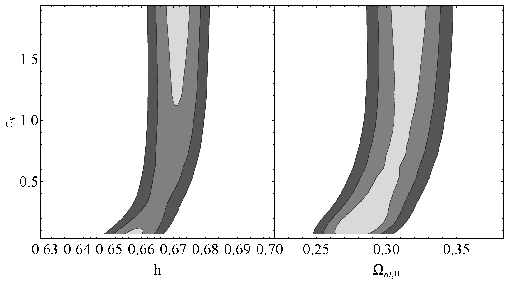
In this Appendix we show some additional contour plots for parameters not shown in the main text.
Figure A1. Gray contours represent the 1 3 σ confidence regions of the Standard Sirens data for the corresponding best fit values (Table 2).
Preprints 76318 g0a1
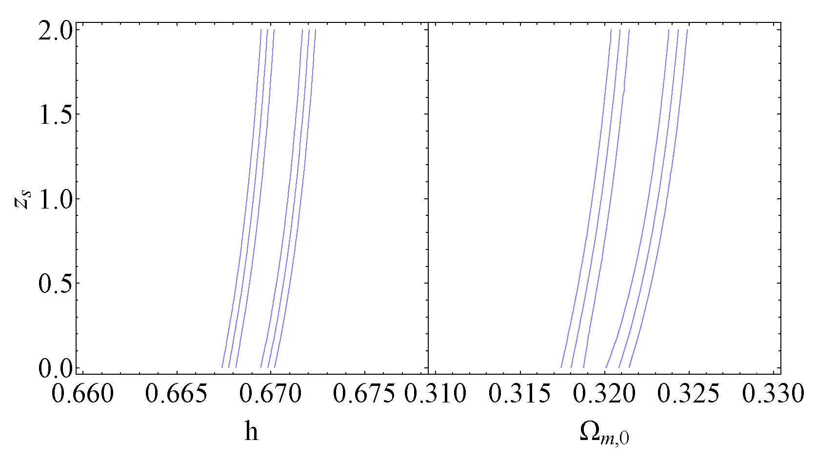
Figure A2. Blue contours represent the projected 1 3 σ confidence regions in h z s , Ω m , 0 z s diagrams of the CMB+BAO data for the sudden leap model (sLCDM), see Table 2.
Preprints 76318 g0a2
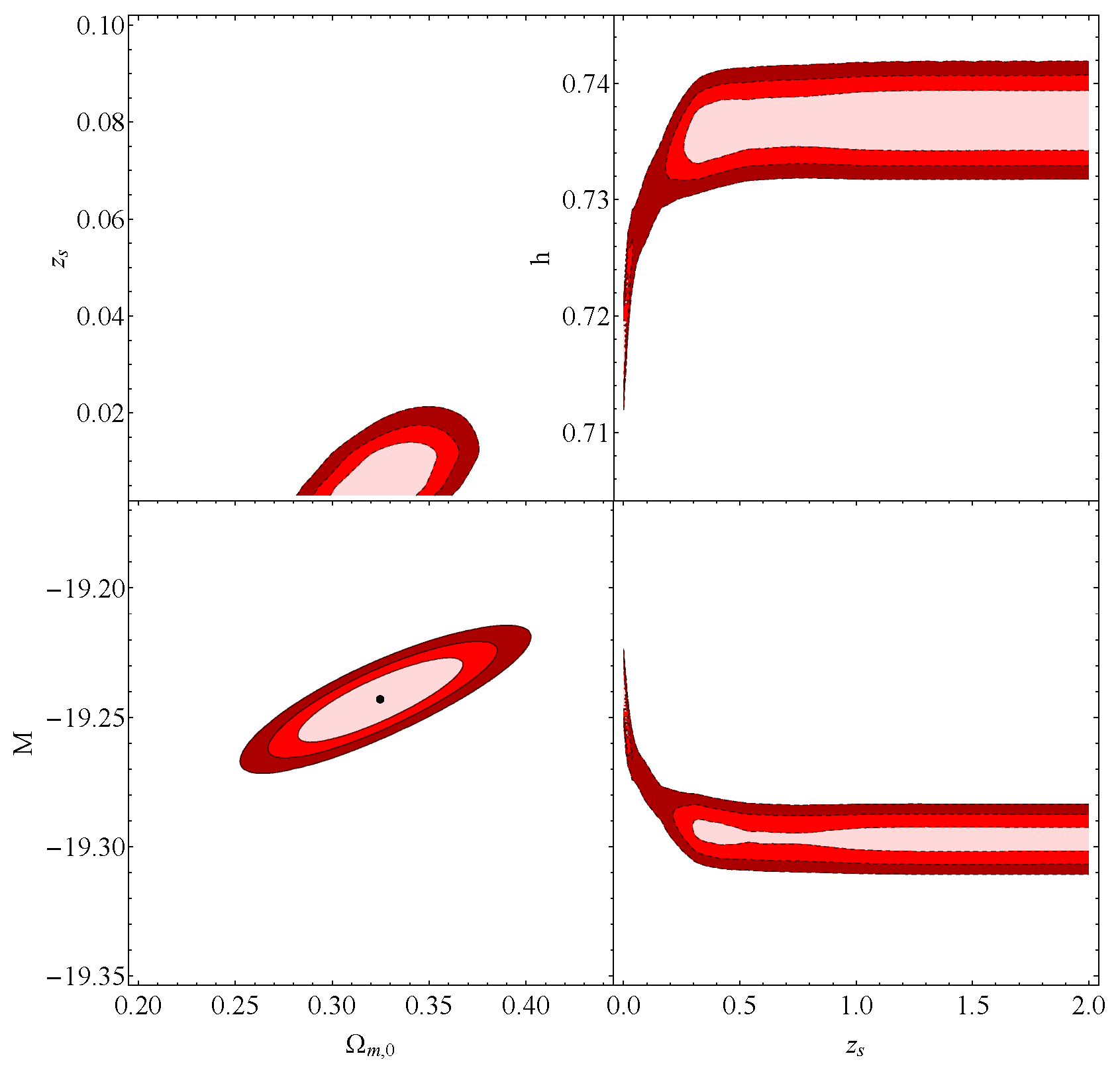
Figure A3. Red contours represent the 1 3 σ confidence regions of the Ω m , 0 z s , Ω m , 0 M , z s M , z s h for the Pantheon+ data and their corresponding best fit values.
Preprints 76318 g0a3
Figure A4. Red contours represent the projected 1 3 σ confidence regions in z s h , z s Ω m , 0 diagrams of the χ 2 = χ sirens 2 + χ BAO 2 + χ Panth 2 + χ CMB 2 distribution, while the gray contours represent the χ 2 = χ BAO 2 + χ Panth 2 + χ CMB 2 .
Preprints 76318 g0a4

Appendix B. Maximum Likelihood Method

A brief overview of the maximum likelihood method is presented. To establish the confidence regions for an unknown parameter in a given distribution, the utilization of the χ 2 distribution is required. Let { x i } denotes a collection of measurements, x o b s represent the associated data vector, and x = x t h e o r y x o b s be the difference between the theoretical and observed data vectors. The χ 2 distribution is defined[102,132,160,161]
χ 2 ( θ ) = x T [ C ] 1 x = [ x i , t h ( θ ) x i , o b s ] ( [ C ] 1 ) i j [ x j , t h ( θ ) x j , o b s ]
Where [ C ] i j C ( x i , x j ) is the covariance and is defined as:
[ C ] = σ 1 2 ρ 12 σ 1 σ 2 ρ 1 n σ 1 σ n ρ 21 σ 1 σ 2 σ 2 2 ρ 2 n σ 2 σ n ρ n 1 σ n σ 1 ρ n 2 σ n σ 2 σ n 2
The likelihood function L of a n dimensional random variable { X i } is defined as L ( { x i } | θ ) = f ( { x i } ; θ ) , where f denotes the corresponding probability density function of { X i } and the unknown parameter θ . In the present context, the likelihood function is
L ( { x i } | θ ) = N e 1 2 χ 2 ( θ )
where N denotes a normalization constant. The likelihood function is used to estimate the most likely "true" parameters θ which are those that sit at a higher value of the likelihood function. In this context, the minimal value of χ 2 distribution, represented as χ m i n 2 χ 2 ( θ ^ ) , aligns with the maximum of the likelihood function. The maximum likelihood estimator θ ^ may exist, it may not and is not necessary to be unique.
By defining the curvature matrix of the likelihood function, the Fisher matrix, is a measure of how rapidly χ 2 variate away from its minimum at the corresponding directions. If the corresponding components of Fisher matrix are large to some directions, then the likelihood changes rapidly and the data are constraining i.e. the resulting uncertainties on the parameters will be small enough. The Fisher matrix is defined:
F i j < 2 ln L θ i θ j >
The Cramer-Rao inequality posits that σ i j ( [ F ] 1 ) i j , and when all parameters are estimated simultaneously, σ θ i ( [ F ] 1 ) i i . In the case that the likelihood is Gaussian, we have σ i j = ( [ F ] 1 ) i j and σ θ i = ( [ F ] 1 ) i i [132,160,161].
When dealing with M parameters in the Fisher matrix and requiring 2D plots, marginalization is applied over the uninteresting parameters ( M 2 parameters). This involves inverting [ F ] and selecting the rows and columns corresponding to the desired parameters, then inverting the resulting "projected" submatrix [53,161].
When the Fisher matrix is singular, no inverse exists, precluding marginalization. Singularity of the Fisher matrix implies a linear combination of two or more parameters in the likelihood. For degenerate parameters, θ 1 , θ 2 , we postulate a new parameter Θ = a θ 1 + b θ 2 to avoid singularity. Notably, a particular case of interest arises when there is a high degree of degeneracy between the two corresponding parameters, referred to as quasi degeneracy. In such situations, a subsequent redefinition of the parameters could once again be necessitated.
The confidence regions live in a parameter space and by projecting them in 2-D, their mappings are confidence "ellipses". We use the confidence regions that correspond to 68.27%, 95.45%, 99.73% percentage of the total probability distribution. For example, a confidence region of 95.45% for θ means that, if we repeat many many times the collection of the data and if for each sample we calculate the confidence region of 95.45% for θ , by computing
θ θ + d θ L ( { x i } | θ ) P ( θ ) P ( { x i } ) = 0.9545
where θ , θ + correspond to the values on either side of each maximum θ ^ and have the same probability. Then, 95.45% of the confidence regions will contain the true value of θ . The confidence regions are those that "moving" as they depend on the corresponding collection of data that are chosen each time.
The one-to-one correspondence between L and χ 2 helps us to estimate the best-fit values for the parameters of interest and also to define the confidence regions around the best-fit values of the corresponding parameters. A fixed Δ χ 2 corresponds to a certain confidence region in parameter space M.
The corresponding Δ χ 2 for a parameter space M of 3-5 dimensions could be seen below:
Δ χ n σ 2
d i m ( M ) 68.27% 95.45% 99.73%
3 3.52674 8.02488 14.1564
4 4.71947 9.71563 16.2513
5 5.8876 11.3139 18.2053
The projected confidence regions are generated by the intervals of the form χ m i n 2 ± Δ χ n σ 2 . In the direction of constraining the data, we demonstrate a schematic overview of the procedure[102]:
C o v a r i a n c e M a t r i x F i s h e r F o r e c a s t P a r a m e t e r C o n s t r a i n t s

Appendix C. ΛCDM model

Here, we present a concise summary of the constraints and the corresponding accuracy obtained through the data analysis performed for the Λ CDM model.
Table A1. χ 2 distributions and the best fit parameters can be seen below: 
Sirens CMB +BAO Pantheon+ Standrad Sirens+Pantheon+ CMB+BAO+Pantheon+ Sirens+CMB+BAO+Pantheon+
1015.07 6.39 1522.98 2575.73 1570.97 2586.54
Data: M Ω m , 0 h
Standard Sirens 0.305 ±0.019 0.676 ± 0.006
CMB +BAO 0.318 ± 0.006 0.672± 0.004
Pantheon+ -19.25± 0.03 0.333 ±0.018 0.734± 0.01
Standard Sirens+Pantheon+ -19.41± 0.01 0.298 ± 0.012 0.683± 0.004
CMB +BAO+Pantheon+ -19.43± 0.01 0.31 ± 0.005 0.677±0.004
CMB+BAO+Pantheon++Standard Sirens -19.43± 0.01 0.311 ± 0.004 0.676± 0.003
Table A2. Accuracy at the ΛCDM model [80]:
Data: Δ M M Δ Ω m , 0 Ω m , 0 Δ h h
Standard Sirens 6.2% 0.9%
CMB +BAO 1.9% 0.6%
Pantheon+ 0.2% 5.4% 1.4%
Standard Sirens+Pantheon+ 0.1% 4.0% 0.6%
CMB +BAO+Pantheon+ 0.1% 1.6% 0.6%
Standard Sirens+CMB+BAO+Pantheon+ 0.1% 1.6% 0.4%

References

  1. Aghanim, N.; et al. Planck 2018 results. VI. Cosmological parameters. Astron. Astrophys. 2020, 641, A6, Erratum: Astron. Astrophys. [Google Scholar] [CrossRef]
  2. Aghanim, N.; et al. Planck 2018 results. III. High Frequency Instrument data processing and frequency maps. Astron. Astrophys. 2020, 641, A3. [Google Scholar] [CrossRef]
  3. Aghanim, N.; et al. Planck 2018 results. I. Overview and the cosmological legacy of Planck. Astron. Astrophys. 2020, 641, A1. [Google Scholar] [CrossRef]
  4. Akrami, Y.; et al. Planck 2018 results. VII. Isotropy and Statistics of the CMB. Astron. Astrophys. 2020, 641, A7. [Google Scholar] [CrossRef]
  5. Akrami, Y.; et al. Planck 2018 results. IX. Constraints on primordial non-Gaussianity. Astron. Astrophys. 2020, 641, A9. [Google Scholar] [CrossRef]
  6. Aghanim, N.; et al. Planck 2018 results. V. CMB power spectra and likelihoods. Astron. Astrophys. 2020, 641, A5. [Google Scholar] [CrossRef]
  7. Akrami, Y.; et al. Planck intermediate results. LVI. Detection of the CMB dipole through modulation of the thermal Sunyaev-Zeldovich effect: Eppur si muove II. Astron. Astrophys. 2020, 644, A100. [Google Scholar] [CrossRef]
  8. Perivolaropoulos, L.; Skara, F. Challenges for ΛCDM: An update. New Astron. Rev. 2022, 95, 101659. [Google Scholar] [CrossRef]
  9. Di Valentino, E. A combined analysis of the H0 late time direct measurements and the impact on the Dark Energy sector. Mon. Not. Roy. Astron. Soc. 2021, 502, 2065–2073. [Google Scholar] [CrossRef]
  10. Riess, A.G.; et al. A Comprehensive Measurement of the Local Value of the Hubble Constant with 1 km s-1 Mpc-1 Uncertainty from the Hubble Space Telescope and the SH0ES Team. Astrophys. J. Lett. 2022, 934, L7. [Google Scholar] [CrossRef]
  11. Perivolaropoulos, L.; Skara, F. A Reanalysis of the Latest SH0ES Data for H0: Effects of New Degrees of Freedom on the Hubble Tension. Universe 2022, 8, 502. [Google Scholar] [CrossRef]
  12. Karwal, T.; Kamionkowski, M. Dark energy at early times, the Hubble parameter, and the string axiverse. Phys. Rev. D 2016, 94, 103523. [Google Scholar] [CrossRef]
  13. Poulin, V.; Smith, T.L.; Karwal, T.; Kamionkowski, M. Early Dark Energy Can Resolve The Hubble Tension. Phys. Rev. Lett. 2019, 122, 221301. [Google Scholar] [CrossRef]
  14. Smith, T.L.; Poulin, V.; Amin, M.A. Oscillating scalar fields and the Hubble tension: A resolution with novel signatures. Phys. Rev. D 2020, 101, 063523. [Google Scholar] [CrossRef]
  15. Niedermann, F.; Sloth, M.S. New early dark energy. Phys. Rev. D 2021, 103, L041303. [Google Scholar] [CrossRef]
  16. Herold, L.; Ferreira, E.G.M. Resolving the Hubble tension with Early Dark Energy 2022. arXiv 2022, arXiv:astro-ph.CO/2210.16296. [Google Scholar]
  17. Abdalla, E.; et al. Cosmology intertwined: A review of the particle physics, astrophysics, and cosmology associated with the cosmological tensions and anomalies. JHEAp 2022, 34, 49–211. [Google Scholar] [CrossRef]
  18. Poulin, V.; Smith, T.L.; Karwal, T. The Ups and Downs of Early Dark Energy solutions to the Hubble tension: a review of models, hints and constraints circa 2023 2023. arXiv 2023, arXiv:astro-ph.CO/2302.09032. [Google Scholar]
  19. Bernal, J.L.; Verde, L.; Riess, A.G. The trouble with H0. JCAP 2016, 10, 019. [Google Scholar] [CrossRef]
  20. Aylor, K.; Joy, M.; Knox, L.; Millea, M.; Raghunathan, S.; Wu, W.L.K. Sounds Discordant: Classical Distance Ladder & ΛCDM -based Determinations of the Cosmological Sound Horizon. Astrophys. J. 2019, 874, 4. [Google Scholar] [CrossRef]
  21. Vagnozzi, S. Consistency tests of ΛCDM from the early integrated Sachs-Wolfe effect: Implications for early-time new physics and the Hubble tension. Phys. Rev. D 2021, 104, 063524. [Google Scholar] [CrossRef]
  22. Hill, J.C.; et al. Atacama Cosmology Telescope: Constraints on prerecombination early dark energy. Phys. Rev. D 2022, 105, 123536. [Google Scholar] [CrossRef]
  23. Brieden, S.; Gil-Marín, H.; Verde, L. A tale of two (or more) h’s 2022. arXiv 2022, arXiv:astro-ph.CO/2212.04522. [Google Scholar]
  24. Bernal, J.L.; Verde, L.; Jimenez, R.; Kamionkowski, M.; Valcin, D.; Wandelt, B.D. The trouble beyond H0 and the new cosmic triangles. Phys. Rev. D 2021, 103, 103533. [Google Scholar] [CrossRef]
  25. Wang, D.; Yan, Y.J.; Meng, X.H. A new pressure-parametrization unified dark fluid model. Eur. Phys. J. C 2017, 77, 263. [Google Scholar] [CrossRef]
  26. Yang, W.; Pan, S.; Di Valentino, E.; Paliathanasis, A.; Lu, J. Challenging bulk viscous unified scenarios with cosmological observations. Phys. Rev. D 2019, 100, 103518. [Google Scholar] [CrossRef]
  27. Cai, R.G.; Guo, Z.K.; Li, L.; Wang, S.J.; Yu, W.W. Chameleon dark energy can resolve the Hubble tension. Phys. Rev. D 2021, 103, 121302. [Google Scholar] [CrossRef]
  28. Li, X.; Shafieloo, A. A Simple Phenomenological Emergent Dark Energy Model can Resolve the Hubble Tension. Astrophys. J. Lett. 2019, 883, L3. [Google Scholar] [CrossRef]
  29. Di Valentino, E.; Mukherjee, A.; Sen, A.A. Dark Energy with Phantom Crossing and the H0 Tension. Entropy 2021, 23, 404. [Google Scholar] [CrossRef]
  30. Di Valentino, E.; Linder, E.V.; Melchiorri, A. H0 ex machina: Vacuum metamorphosis and beyond H0. Phys. Dark Univ. 2020, 30, 100733. [Google Scholar] [CrossRef]
  31. Benevento, G.; Kable, J.A.; Addison, G.E.; Bennett, C.L. An Exploration of an Early Gravity Transition in Light of Cosmological Tensions. Astrophys. J. 2022, 935, 156. [Google Scholar] [CrossRef]
  32. Heisenberg, L.; Villarrubia-Rojo, H.; Zosso, J. Simultaneously solving the H0 and σ8 tensions with late dark energy. Phys. Dark Univ. 2023, 39, 101163. [Google Scholar] [CrossRef]
  33. Hernández-Almada, A.; Leon, G.; Magaña, J.; García-Aspeitia, M.A.; Motta, V.; Saridakis, E.N.; Yesmakhanova, K. Kaniadakis-holographic dark energy: observational constraints and global dynamics. Mon. Not. Roy. Astron. Soc. 2022, 511, 4147–4158. [Google Scholar] [CrossRef]
  34. Alestas, G.; Perivolaropoulos, L. Late-time approaches to the Hubble tension deforming H(z), worsen the growth tension. Mon. Not. Roy. Astron. Soc. 2021, 504, 3956–3962. [Google Scholar] [CrossRef]
  35. Benevento, G.; Hu, W.; Raveri, M. Can Late Dark Energy Transitions Raise the Hubble constant? Phys. Rev. D 2020, 101, 103517. [Google Scholar] [CrossRef]
  36. Alestas, G.; Camarena, D.; Di Valentino, E.; Kazantzidis, L.; Marra, V.; Nesseris, S.; Perivolaropoulos, L. Late-transition versus smooth H(z)-deformation models for the resolution of the Hubble crisis. Phys. Rev. D 2022, 105, 063538. [Google Scholar] [CrossRef]
  37. Yang, W.; Di Valentino, E.; Pan, S.; Wu, Y.; Lu, J. Dynamical dark energy after Planck CMB final release and H 0 tension. Monthly Notices of the Royal Astronomical Society 2020, 501. [Google Scholar] [CrossRef]
  38. Marra, V.; Perivolaropoulos, L. Rapid transition of Geff at zt≃0.01 as a possible solution of the Hubble and growth tensions. Phys. Rev. D 2021, 104, L021303. [Google Scholar] [CrossRef]
  39. Alestas, G.; Kazantzidis, L.; Perivolaropoulos, L. w-M phantom transition at zt<0.1 as a resolution of the Hubble tension. Phys. Rev. D 2021, 103, 083517. [Google Scholar] [CrossRef]
  40. Perivolaropoulos, L.; Skara, F. On the homogeneity of SnIa absolute magnitude in the Pantheon+ sample 2023. arXiv 2023, arXiv:astro-ph.CO/2301.01024. [Google Scholar]
  41. Alestas, G.; Antoniou, I.; Perivolaropoulos, L. Hints for a Gravitational Transition in Tully–Fisher Data. Universe 2021, 7, 366. [Google Scholar] [CrossRef]
  42. Perivolaropoulos, L. Is the Hubble Crisis Connected with the Extinction of Dinosaurs? Universe 2022, 8, 263. [Google Scholar] [CrossRef]
  43. Alestas, G.; Perivolaropoulos, L.; Tanidis, K. Constraining a late time transition of Geff using low-z galaxy survey data. Phys. Rev. D 2022, 106, 023526. [Google Scholar] [CrossRef]
  44. Perivolaropoulos, L.; Skara, F. Hubble tension or a transition of the Cepheid SnIa calibrator parameters? Phys. Rev. D 2021, 104, 123511. [Google Scholar] [CrossRef]
  45. Perivolaropoulos, L.; Skara, F. Gravitational transitions via the explicitly broken symmetron screening mechanism. Phys. Rev. D 2022, 106, 043528. [Google Scholar] [CrossRef]
  46. Lee, W.; Lee, B.H.; Lee, C.H.; Park, C. The False vacuum bubble nucleation due to a nonminimally coupled scalar field. Phys. Rev. D 2006, 74, 123520. [Google Scholar] [CrossRef]
  47. Barrow, J.D. Sudden future singularities. Classical and Quantum Gravity 2004, 21, L79–L82. [Google Scholar] [CrossRef]
  48. Barrow, J.D.; Tsagas, C.G. New isotropic and anisotropic sudden singularities. Class. Quant. Grav. 2005, 22, 1563–1571. [Google Scholar] [CrossRef]
  49. Fernandez-Jambrina, L.; Lazkoz, R. Geodesic Completeness around Sudden Singularities. AIP Conf. Proc. 2006, 841, 420. [Google Scholar] [CrossRef]
  50. Fernandez-Jambrina, L.; Lazkoz, R. Singular fate of the universe in modified theories of gravity. Phys. Lett. B 2009, 670, 254–258. [Google Scholar] [CrossRef]
  51. Fernandez-Jambrina, L.; Lazkoz, R. Classification of cosmological milestones. Phys. Rev. D 2006, 74, 064030. [Google Scholar] [CrossRef]
  52. Perivolaropoulos, L. Fate of bound systems through sudden future singularities. Phys. Rev. D 2016, 94, 124018. [Google Scholar] [CrossRef]
  53. Amendola, L.; Tsujikawa, S. Dark Energy: Theory and Observations; Cambridge University Press, 2010. [CrossRef]
  54. Cattoën, C.; Visser, M. Necessary and sufficient conditions for big bangs, bounces, crunches, rips, sudden singularities and extremality events. Classical and Quantum Gravity 2005, 22, 4913–4930. [Google Scholar] [CrossRef]
  55. Barrow, J.D. More general sudden singularities. Class. Quant. Grav. 2004, 21, 5619–5622. [Google Scholar] [CrossRef]
  56. Denkiewicz, T.; Dą browski, M.P.; Ghodsi, H.; Hendry, M.A. Cosmological tests of sudden future singularities. Physical Review D 2012, 85. [Google Scholar] [CrossRef]
  57. Bamba, K.; Nojiri, S. The future of the universe in modified gravitational theories: Approaching a finite-time future singularity. Journal of Cosmology and Astroparticle Physics 2008, 2008. [Google Scholar] [CrossRef]
  58. Bamba, K.; Capozziello, S.; Nojiri, S.; Odintsov, S.D. Dark energy cosmology: the equivalent description via different theoretical models and cosmography tests. Astrophys. Space Sci. 2012, 342, 155–228. [Google Scholar] [CrossRef]
  59. Caldwell, R.R.; Kamionkowski, M.; Weinberg, N.N. Phantom energy and cosmic doomsday. Phys. Rev. Lett. 2003, 91, 071301. [Google Scholar] [CrossRef]
  60. Nojiri, S.; Odintsov, S.D.; Tsujikawa, S. Properties of singularities in the (phantom) dark energy universe. Physical Review D 2005, 71. [Google Scholar] [CrossRef]
  61. Stefancic, H. Expansion around the vacuum equation of state - Sudden future singularities and asymptotic behavior. Phys. Rev. D 2005, 71, 084024. [Google Scholar] [CrossRef]
  62. Nojiri, S.; Odintsov, S.D. The Final state and thermodynamics of dark energy universe. Phys. Rev. D 2004, 70, 103522. [Google Scholar] [CrossRef]
  63. Dąbrowski, M.P.; Denkiewicz, T. Barotropic index w-singularities in cosmology. Phys. Rev. D 2009, 79, 063521. [Google Scholar] [CrossRef]
  64. Frampton, P.H.; Ludwick, K.J.; Scherrer, R.J. The little rip. Physical Review D 2011, 84. [Google Scholar] [CrossRef]
  65. Frampton, P.H.; Ludwick, K.J.; Scherrer, R.J. Pseudo-rip: Cosmological models intermediate between the cosmological constant and the little rip. Physical Review D 2012, 85. [Google Scholar] [CrossRef]
  66. Clarke, C.; Królak, A. Conditions for the occurence of strong curvature singularities. Journal of Geometry and Physics 1985, 2, 127–143. [Google Scholar] [CrossRef]
  67. Tipler, F.J. Singularities in conformally flat spacetimes. Phys. Lett. A 1977, 64, 8–10. [Google Scholar] [CrossRef]
  68. Fernandez-Jambrina, L.; Lazkoz, R. Geodesic Behaviour around Cosmological Milestones. J. Phys. Conf. Ser. 2007, 66, 012015. [Google Scholar] [CrossRef]
  69. Gaztanaga, E.; Garcia-Berro, E.; Isern, J.; Bravo, E.; Dominguez, I. Bounds on the possible evolution of the Gravitational Constant from Cosmological Type-Ia Supernovae. Physical Review D 2001, 65. [Google Scholar] [CrossRef]
  70. Vijaykumar, A.; Kapadia, S.J.; Ajith, P. Constraints on the Time Variation of the Gravitational Constant Using Gravitational Wave Observations of Binary Neutron Stars. Physical Review Letters 2021, 126. [Google Scholar] [CrossRef]
  71. Uzan, J.P. The fundamental constants and their variation: observational and theoretical status. Reviews of Modern Physics 2003, 75, 403–455. [Google Scholar] [CrossRef]
  72. Conselice, C.; Bundy, K.; Ellis, R.; Brichmann, J.; Vogt, N.; Phillips, A. Evolution of the Near-Infrared Tully-Fisher Relation: Constraints on the Relationship Between the Stellar and Total Masses of Disk Galaxies since z=1. The Astrophysical Journal 2005, 628. [Google Scholar] [CrossRef]
  73. Alvey, J.; Sabti, N.; Escudero, M.; Fairbairn, M. Improved BBN Constraints on the Variation of the Gravitational Constant. Eur. Phys. J. C 2020, 80, 148. [Google Scholar] [CrossRef]
  74. Wu, F.; Chen, X. Cosmic microwave background with Brans-Dicke gravity II: constraints with the WMAP and SDSS data. Phys. Rev. D 2010, 82, 083003. [Google Scholar] [CrossRef]
  75. Punturo, M.; et al. The Einstein Telescope: A third-generation gravitational wave observatory. Class. Quant. Grav. 2010, 27, 194002. [Google Scholar] [CrossRef]
  76. Sathyaprakash, B.; et al. Scientific Objectives of Einstein Telescope. Class. Quant. Grav. 2012, 29, 124013, Erratum: Class. Quant. Grav. 2013, 30, 079501. [Google Scholar] [CrossRef]
  77. Zhao, W.; Broeck, C.V.D.; Baskaran, D.; Li, T.G.F. Determination of dark energy by the Einstein Telescope: Comparing with CMB, BAO, and SNIa observations. Physical Review D 2011, 83. [Google Scholar] [CrossRef]
  78. Taylor, S.R.; Gair, J.R. Cosmology with the lights off: standard sirens in the Einstein Telescope era. Phys. Rev. D 2012, 86, 023502. [Google Scholar] [CrossRef]
  79. D’Agostino, R.; Nunes, R.C. Probing observational bounds on scalar-tensor theories from standard sirens. Phys. Rev. D 2019, 100, 044041. [Google Scholar] [CrossRef]
  80. Belgacem, E.; Dirian, Y.; Foffa, S.; Maggiore, M. Modified gravitational-wave propagation and standard sirens. Physical Review D 2018, 98. [Google Scholar] [CrossRef]
  81. Maggiore, M.; et al. Science Case for the Einstein Telescope. JCAP 2020, 03, 050. [Google Scholar] [CrossRef]
  82. Branchesi, M.; et al. Science with the Einstein Telescope: a comparison of different designs 2023. arXiv 2023, arXiv:gr-qc/2303.15923. [Google Scholar]
  83. Abbott, B.P.; et al. Prospects for observing and localizing gravitational-wave transients with Advanced LIGO, Advanced Virgo and KAGRA. Living Rev. Rel. 2018, 21, 3. [Google Scholar] [CrossRef]
  84. Aasi, J.; et al. Advanced LIGO. Class. Quant. Grav. 2015, 32, 074001. [Google Scholar] [CrossRef]
  85. Acernese, F.; et al. Advanced Virgo: a second-generation interferometric gravitational wave detector. Class. Quant. Grav. 2015, 32, 024001. [Google Scholar] [CrossRef]
  86. Aso, Y.; Michimura, Y.; Somiya, K.; Ando, M.; Miyakawa, O.; Sekiguchi, T.; Tatsumi, D.; Yamamoto, H. Interferometer design of the KAGRA gravitational wave detector. Phys. Rev. D 2013, 88, 043007. [Google Scholar] [CrossRef]
  87. Will, C.M. THE CONFRONTATION BETWEEN GENERAL RELATIVITY AND EXPERIMENT: AN UPDATE. Phys. Rept. 1984, 113, 345–422. [Google Scholar] [CrossRef]
  88. Boisseau, B.; Esposito-Farese, G.; Polarski, D.; Starobinsky, A.A. Reconstruction of a scalar tensor theory of gravity in an accelerating universe. Phys. Rev. Lett. 2000, 85, 2236. [Google Scholar] [CrossRef] [PubMed]
  89. Esposito-Farese, G.; Polarski, D. Scalar tensor gravity in an accelerating universe. Phys. Rev. D 2001, 63, 063504. [Google Scholar] [CrossRef]
  90. Perivolaropoulos, L. Crossing the phantom divide barrier with scalar tensor theories. JCAP 2005, 10, 001. [Google Scholar] [CrossRef]
  91. Nishizawa, A. Generalized framework for testing gravity with gravitational-wave propagation. I. Formulation. Physical Review D 2018, 97. [Google Scholar] [CrossRef]
  92. Arai, S.; Nishizawa, A. Generalized framework for testing gravity with gravitational-wave propagation. II. Constraints on Horndeski theory. Phys. Rev. D 2018, 97, 104038. [Google Scholar] [CrossRef]
  93. Linder, E.V. No slip gravity. Journal of Cosmology and Astroparticle Physics 2018, 2018, 005–005. [Google Scholar] [CrossRef]
  94. Eardley, D.M.; Lee, D.L.; Lightman, A.P. Gravitational-wave observations as a tool for testing relativistic gravity. Phys. Rev. D 1973, 8, 3308–3321. [Google Scholar] [CrossRef]
  95. Belgacem, E.; Dirian, Y.; Foffa, S.; Maggiore, M. Gravitational-wave luminosity distance in modified gravity theories. Phys. Rev. D 2018, 97, 104066. [Google Scholar] [CrossRef]
  96. Maggiore, M. Gravitational Waves: Volume 1: Theory and Experiments; Oxford University Press, 2007. [CrossRef]
  97. Maggiore, M. Gravitational Waves: Volume 2: Astrophysics and Cosmology; Oxford University Press, 2018. [CrossRef]
  98. Nishizawa, A. Generalized framework for testing gravity with gravitational-wave propagation. I. Formulation. Phys. Rev. D 2018, 97, 104037. [Google Scholar] [CrossRef]
  99. Oikonomou, V.; Myrzakulov, R. Spectrum of Primordial Gravitational Waves in Modified Gravities: A Short Overview. Symmetry 2022, 14, 729. [Google Scholar] [CrossRef]
  100. de Matos, I.; Calvão, M.; Waga, I. Gravitational wave propagation in f ( R ) models: New parametrizations and observational constraints. Physical Review D 2021, 103. [Google Scholar] [CrossRef]
  101. Tasinato, G.; Garoffolo, A.; Bertacca, D.; Matarrese, S. Gravitational-wave cosmological distances in scalar-tensor theories of gravity. JCAP 2021, 06, 050. [Google Scholar] [CrossRef]
  102. Dodelson, S.; Schmidt, F. Modern Cosmology; Elsevier Science, 2020.
  103. Arfken, G.; Weber, H.; Harris, F. Mathematical Methods for Physicists: A Comprehensive Guide; Elsevier Science, 2012.
  104. Saltas, I.D.; Sawicki, I.; Amendola, L.; Kunz, M. Anisotropic Stress as a Signature of Nonstandard Propagation of Gravitational Waves. Phys. Rev. Lett. 2014, 113, 191101. [Google Scholar] [CrossRef] [PubMed]
  105. Pettorino, V.; Amendola, L. Friction in Gravitational Waves: a test for early-time modified gravity. Phys. Lett. B 2015, 742, 353–357. [Google Scholar] [CrossRef]
  106. Gleyzes, J.; Langlois, D.; Vernizzi, F. A unifying description of dark energy. Int. J. Mod. Phys. D 2015, 23, 1443010. [Google Scholar] [CrossRef]
  107. Belgacem, E.; Calcagni, G.; Crisostomi, M.; Dalang, C.; Dirian, Y.; Ezquiaga, J.M.; Fasiello, M.; Foffa, S.; Ganz, A.; García-Bellido, J.; et al. Testing modified gravity at cosmological distances with LISA standard sirens. Journal of Cosmology and Astroparticle Physics 2019, 2019, 024–024. [Google Scholar] [CrossRef]
  108. Cai, R.G.; Liu, T.B.; Liu, X.W.; Wang, S.J.; Yang, T. Probing cosmic anisotropy with gravitational waves as standard sirens. Phys. Rev. D 2018, 97, 103005. [Google Scholar] [CrossRef]
  109. Yang, W.; Pan, S.; Di Valentino, E.; Escamilla-Rivera, C.; Paliathanasis, A. Exploring bulk viscous unified scenarios with Gravitational Waves Standard Sirens 2023. arXiv, 2023. [Google Scholar] [CrossRef]
  110. Fu, X.; Zhou, L.; Chen, J. Testing the cosmic distance-duality relation from future gravitational wave standard sirens. Phys. Rev. D 2019, 99, 083523. [Google Scholar] [CrossRef]
  111. Cai, R.G.; Yang, T. Space-borne atom interferometric gravitational wave detections. Part I. The forecast of bright sirens on cosmology. JCAP 2021, 12, 017. [Google Scholar] [CrossRef]
  112. Mukherjee, S.; Wandelt, B.D.; Silk, J. Testing the general theory of relativity using gravitational wave propagation from dark standard sirens. Mon. Not. Roy. Astron. Soc. 2021, 502, 1136–1144. [Google Scholar] [CrossRef]
  113. Auclair, P.; et al. Cosmology with the Laser Interferometer Space Antenna 2022. arXiv 2022, arXiv:astro-ph.CO/2204.05434. [Google Scholar]
  114. Abbott, B.P.; et al. Exploring the Sensitivity of Next Generation Gravitational Wave Detectors. Class. Quant. Grav. 2017, 34, 044001. [Google Scholar] [CrossRef]
  115. Zhang, X. Gravitational wave standard sirens and cosmological parameter measurement. Sci. China Phys. Mech. Astron. 2019, 62, 110431. [Google Scholar] [CrossRef]
  116. Califano, M.; de Martino, I.; Vernieri, D.; Capozziello, S. Exploiting the Einstein Telescope to solve the Hubble tension. arXiv 2022. [Google Scholar] [CrossRef]
  117. Schutz, B.F. Determining the Hubble constant from gravitational wave observations. Nature 1986, 323, 310–311. [Google Scholar] [CrossRef]
  118. Abbott, B.P.; et al. A gravitational-wave standard siren measurement of the Hubble constant. Nature 2017, 551, 85–88. [Google Scholar]
  119. Chen, H.Y.; Fishbach, M.; Holz, D.E. A two per cent Hubble constant measurement from standard sirens within five years. Nature 2021, 592, 71–76. [Google Scholar] [CrossRef]
  120. Khan, S.; Husa, S.; Hannam, M.; Ohme, F.; Pürrer, M.; Jiménez Forteza, X.; Bohé, A. Frequency-domain gravitational waves from nonprecessing black-hole binaries. II. A phenomenological model for the advanced detector era. Phys. Rev. D 2016, 93, 044007. [Google Scholar] [CrossRef]
  121. Breschi, M.; Bernuzzi, S.; Chakravarti, K.; Camilletti, A.; Prakash, A.; Perego, A. Kilohertz Gravitational Waves From Binary Neutron Star Mergers: Numerical-relativity Informed Postmerger Model. arXiv 2022, arXiv:gr-qc/2205.09112. [Google Scholar]
  122. Breschi, M.; Gamba, R.; Borhanian, S.; Carullo, G.; Bernuzzi, S. Kilohertz Gravitational Waves from Binary Neutron Star Mergers: Inference of Postmerger Signals with the Einstein Telescope. arXiv 2022, arXiv:gr-qc/2205.09979. [Google Scholar]
  123. Nagar, A.; Bernuzzi, S.; Pozzo, W.; Riemenschneider, G.; Akcay, S.; Carullo, G.; Fleig, P.; Babak, S.; Tsang, K.; Colleoni, M.; et al. Time-domain effective-one-body gravitational waveforms for coalescing compact binaries with nonprecessing spins, tides, and self-spin effects. Physical Review D 2018, 98. [Google Scholar] [CrossRef]
  124. Estellés, H.; Colleoni, M.; García-Quirós, C.; Husa, S.; Keitel, D.; Mateu-Lucena, M.; Planas, M.d.L.; Ramos-Buades, A. New twists in compact binary waveform modeling: A fast time-domain model for precession. Phys. Rev. D 2022, 105, 084040. [Google Scholar] [CrossRef]
  125. Zhao, W.; Van Den Broeck, C.; Baskaran, D.; Li, T.G.F. Determination of Dark Energy by the Einstein Telescope: Comparing with CMB, BAO and SNIa Observations. Phys. Rev. D 2011, 83, 023005. [Google Scholar] [CrossRef]
  126. Sathyaprakash, B.S.; Schutz, B.F.; Van Den Broeck, C. Cosmography with the Einstein Telescope. Class. Quant. Grav. 2010, 27, 215006. [Google Scholar] [CrossRef]
  127. Belgacem, E.; Dirian, Y.; Foffa, S.; Maggiore, M. Gravitational-wave luminosity distance in modified gravity theories. Phys. Rev. D 2018, 97, 104066. [Google Scholar] [CrossRef]
  128. Eisenstein, D.J.; Hu, W. Baryonic features in the matter transfer function. Astrophys. J. 1998, 496, 605. [Google Scholar] [CrossRef]
  129. Kazantzidis, L.; Perivolaropoulos, L.; Skara, F. Constraining power of cosmological observables: Blind redshift spots and optimal ranges. Physical Review D 2019, 99. [Google Scholar] [CrossRef]
  130. Eisenstein, D.J.; et al. Detection of the Baryon Acoustic Peak in the Large-Scale Correlation Function of SDSS Luminous Red Galaxies. Astrophys. J. 2005, 633, 560–574. [Google Scholar] [CrossRef]
  131. Hu, W.; Sugiyama, N. Small scale cosmological perturbations: An Analytic approach. Astrophys. J. 1996, 471, 542–570. [Google Scholar] [CrossRef]
  132. Theodoropoulos, A.; Perivolaropoulos, L. The Hubble Tension, the M Crisis of Late Time H(z) Deformation Models and the Reconstruction of Quintessence Lagrangians. Universe 2021, 7, 300. [Google Scholar] [CrossRef]
  133. Zhai, Z.; Wang, Y. Robust and model-independent cosmological constraints from distance measurements. JCAP 2019, 07, 005. [Google Scholar] [CrossRef]
  134. Escamilla-Rivera, C. Status on Bidimensional Dark Energy Parameterizations Using SNe Ia JLA and BAO Datasets. Galaxies 2016, 4, 8. [Google Scholar] [CrossRef]
  135. Jones, D.; Saunders, W.; Colless, M.; Read, M.; Parker, Q.; Watson, F.; Campbell, L.; Burkey, D.; Mauch, T.; Moore, L.; et al. The 6dF Galaxy Survey: Samples, Observational Techniques and the First Data Release. Monthly Notices of the Royal Astronomical Society 2004, 355, 747–763. [Google Scholar] [CrossRef]
  136. Drinkwater, M.J.; et al. The WiggleZ Dark Energy Survey: Survey Design and First Data Release. Mon. Not. Roy. Astron. Soc. 2010, 401, 1429–1452. [Google Scholar] [CrossRef]
  137. Gaztanaga, E.; Garcia-Berro, E.; Isern, J.; Bravo, E.; Dominguez, I. Bounds on the possible evolution of the gravitational constant from cosmological type Ia supernovae. Phys. Rev. D 2002, 65, 023506. [Google Scholar] [CrossRef]
  138. Brout, D.; et al. The Pantheon+ Analysis: Cosmological Constraints. Astrophys. J. 2022, 938, 110. [Google Scholar] [CrossRef]
  139. Scolnic, D.M.; et al. The Complete Light-curve Sample of Spectroscopically Confirmed SNe Ia from Pan-STARRS1 and Cosmological Constraints from the Combined Pantheon Sample. Astrophys. J. 2018, 859, 101. [Google Scholar] [CrossRef]
  140. Perivolaropoulos, L. On the isotropy of SnIa absolute magnitudes in the Pantheon+ and SH0ES samples. arXiv 2023, arXiv:astro-ph.CO/2305.12819. [Google Scholar]
  141. Burnham, K.; Anderson, D. Model Selection and Multimodel Inference: A Practical Information-Theoretic Approach; Springer New York, 2003.
  142. Shi, K.; Huang, Y.; Lu, T. A comprehensive comparison of cosmological models from latest observational data. Mon. Not. Roy. Astron. Soc. 2012, 426, 2452–2462. [Google Scholar] [CrossRef]
  143. Kazantzidis, L.; Perivolaropoulos, L. Hints of a Local Matter Underdensity or Modified Gravity in the Low z Pantheon data. Phys. Rev. D 2020, 102, 023520. [Google Scholar] [CrossRef]
  144. Fernández-Jambrina, L. Singularities in Inflationary Cosmological Models. Universe 2021, 7, 491. [Google Scholar] [CrossRef]
  145. Zhao, W.; Van Den Broeck, C.; Baskaran, D.; Li, T. Determination of Dark Energy by the Einstein Telescope: Comparing with CMB, BAO and SNIa Observations. Physical Review D - PHYS REV D 2010, 83. [Google Scholar] [CrossRef]
  146. Klein, A.; et al. Science with the space-based interferometer eLISA: Supermassive black hole binaries. Phys. Rev. D 2016, 93, 024003. [Google Scholar] [CrossRef]
  147. Tamanini, N.; Caprini, C.; Barausse, E.; Sesana, A.; Klein, A.; Petiteau, A. Science with the space-based interferometer eLISA. III: Probing the expansion of the Universe using gravitational wave standard sirens. Journal of Cosmology and Astroparticle Physics 2016, 2016. [Google Scholar] [CrossRef]
  148. Mangiagli, A.; Caprini, C.; Volonteri, M.; Marsat, S.; Vergani, S.; Tamanini, N.; Inchauspé, H. Massive black hole binaries in LISA: Multimessenger prospects and electromagnetic counterparts. Phys. Rev. D 2022, 106, 103017. [Google Scholar] [CrossRef]
  149. Mangiagli, A.; Caprini, C.; Volonteri, M.; Marsat, S.; Vergani, S.; Tamanini, N.; Speri, L. Cosmology with massive black hole binary mergers in the LISA era. PoS 2022, ICHEP2022, 125. [Google Scholar] [CrossRef]
  150. Amaro-Seoane, P.; et al. Laser Interferometer Space Antenna. arXiv 2017, arXiv:astro-ph.IM/1702.00786. [Google Scholar]
  151. Caprini, C.; et al. Science with the space-based interferometer eLISA. II: Gravitational waves from cosmological phase transitions. JCAP 2016, 04, 001. [Google Scholar] [CrossRef]
  152. Speri, L.; Tamanini, N.; Caldwell, R.; Gair, J.; Wang, B. Testing the quasar Hubble diagram with LISA standard sirens. Physical Review D 2021, 103. [Google Scholar] [CrossRef]
  153. Breivik, K.; Kremer, K.; Bueno, M.; Larson, S.L.; Coughlin, S.; Kalogera, V. Characterizing Accreting Double White Dwarf Binaries with the Laser Interferometer Space Antenna and Gaia. Astrophys. J. Lett. 2018, 854, L1. [Google Scholar] [CrossRef]
  154. Korol, V.; Rossi, E.; Groot, P.; Nelemans, G.; Toonen, S.; Brown, A. Prospects for detection of detached double white dwarf binaries with Gaia, LSST and LISA. Monthly Notices of the Royal Astronomical Society 2017, 470. [Google Scholar] [CrossRef]
  155. Korol, V.; Koop, O.; Rossi, E. Detectability of Double White Dwarfs in the Local Group with LISA. The Astrophysical Journal 2018, 866, L20. [Google Scholar] [CrossRef]
  156. Lau, M.Y.M.; Mandel, I.; Vigna-Gómez, A.; Neijssel, C.J.; Stevenson, S.; Sesana, A. Detecting Double Neutron Stars with LISA. Mon. Not. Roy. Astron. Soc. 2020, 492, 3061–3072. [Google Scholar] [CrossRef]
  157. Sesana, A. Prospects for Multiband Gravitational-Wave Astronomy after GW150914. Phys. Rev. Lett. 2016, 116, 231102. [Google Scholar] [CrossRef]
  158. Babak, S.; Gair, J.; Sesana, A.; Barausse, E.; Sopuerta, C.F.; Berry, C.P.L.; Berti, E.; Amaro-Seoane, P.; Petiteau, A.; Klein, A. Science with the space-based interferometer LISA. V: Extreme mass-ratio inspirals. Phys. Rev. D 2017, 95, 103012. [Google Scholar] [CrossRef]
  159. Caprini, C.; Figueroa, D.G. Cosmological Backgrounds of Gravitational Waves. Class. Quant. Grav. 2018, 35, 163001. [Google Scholar] [CrossRef]
  160. Fortran, I.; Press, W.; Teukolsky, S.; Vetterling, W.; Flannery, B. Numerical Recipes. Cambridge, UK, Cambridge University Press, 1992. [Google Scholar]
  161. Verde, L. Statistical Methods in Cosmology. In Lectures on Cosmology; Springer Berlin Heidelberg, 2010; pp. 147–177. [CrossRef]
1
There is also a completely analogous characterization with the corresponding Tipler integral [67]
2
Some additional contour plots are presented in Appendix A (Figure A1).
3
Some additional contour plots are presented in Appendix A (Figure A2).
4
Some additional contour plots are presented in Appendix A (Figure A3).
5
Some additional contour plots are presented in Appendix A (Figure A4).
Figure 1. There is a transition from a matter dominated phase ( τ < τ s ). The dimensionless τ , is plotted along the x-axis, the following parameters for each case, τ s = 500 , β = 2 3 , σ = 0.1 , a s = 0.995 , are fixed. We chose as initial conditions h c ( τ = 200 ) = 1 and h c ( τ = 200 ) = 0 , just for illustration. The red waveforms corresponds to the gravitational waves after the singularity, in the context of General Relativity ( α M = 0 ) and the blue waveforms corresponds to the propagation of gravitational waves with a modification, that is incorporated by the friction term α M . It is also assumed that Θ ( 0 ) = 1 2 .
Preprints 76318 g001
Figure 2. The long-term effects on the amplitude of the gravitational wave due to friction, as opposed to the initial gravitational wave. This behavior is due to a transition from a matter dominated phase ( τ < τ s ). The dimensionless parameter τ is plotted along the x-axis, and the following parameters are fixed for each case: τ s = 500 , β = 2 3 , σ = 0.1 , a s = 0.995 . To illustrate this behavior, we selected the initial conditions h c ( τ = 200 ) = 1 and h c ( τ = 200 ) = 0 . The red waveforms represent the gravitational waves after the singularity, within the context of General Relativity ( α M = 0 ), while the blue waveforms depict the propagation of gravitational waves with a modification, which is incorporated by the extra friction term α M through gravitational transition. Additionally, we assume that Θ ( 0 ) = 1 2 .
Preprints 76318 g002
Figure 3. Let N 0 be the normalization constant, which is approximately equal to 1.42198 × 10 9 , and let f ( z ) be the number density function (see Figure 8 in Belgacem et al. (2018) or Figure 2 in Zhao et al. (2011)). We define the non-standard cumulative distribution function N ( z ) . To generate a list of non-uniformly distributed z i values, we solve the equation N ( z i ) = i for i = 1 , 2 , , 1000 , where i is an integer.
Preprints 76318 g003
Figure 4. The cosmology model assumed is Λ CDM with Ω m , 0 = 0.3166 and H 0 = 67.27 k m s M p c 1 , the blue curve corresponds to the mean value or else d ¯ L ( z ) = ( 1 + z ) 0 z c H 0 Ω m , 0 ( 1 + z ) 3 + 1 Ω m , 0 d z , while the yellow and red curves correspond to d ¯ L ( z ) ± σ ( z ) respectively (see Figure 7 [80]). The dots constructed are the 1000 standard sirens which are distributed through the relation (43).
Preprints 76318 g004
Figure 5. The black contours on the h α , Ω m , 0 h , and Ω m , 0 h diagrams represent the projected confidence regions, at 1 3 σ , of the Standard Sirens using mock data. These contours correspond to a transition that occurs at the best fit value of a s = 0.401 ± 0.397 and for the corresponding best fit values each time, Ω m , 0 , h , α , which can be found in Table 2.
Preprints 76318 g005
Figure 6. The blue contours in the h α , Ω m , 0 h , and Ω m , 0 h diagrams represent the projected 1 3 σ confidence regions based on the CMB+BAO data for the sudden leap model (sLCDM). The best fit value for the transition occurring at a s = 0.299 ± 0.048 , along with the corresponding best fit values of Ω m , 0 , h, and α , can be found in Table 2.
Preprints 76318 g006
Figure 8. A combined plot including the contours of Figure 5 (Black contours which correspond to the confidence regions of the mock data of the standard sirens for the sudden leap model), Figure 6 (Blue contours which correspond to the confidence regions of the assemblage of C M B , B A O data of the sudden leap model), Figure 7 (Red contours which correspond to the confidence regions of the Pantheon+ data of the sudden leap model), in contrast to one another.
Preprints 76318 g008
Figure 9. The red contours observed in the h α , Ω m , 0 α , and Ω m , 0 h diagrams represent the projected 1 3 σ confidence regions obtained through the analysis of the combined χ 2 function within the sudden leap model (sLCDM). This combined χ 2 function comprises contributions from χ sirens 2 , χ BAO 2 , χ Panth 2 , and χ CMB 2 . The best fit values for the transition occurring at a s = 0.812 ± 0.2 and the absolute magnitude M = 19.43 ± 0.015 , as well as the corresponding best fit values for Ω m , 0 , h, and α , are provided in Table 2. Additionally, the gray contours reflect the contributions from χ BAO 2 , χ CMB 2 and χ Panth 2 for the corresponding best fit values of a s = 0.789 ± 0.2 and M = 19.43 ± 0.015 .
Preprints 76318 g009
Figure 10. The resulting red contours which correspond to the confidence regions of the Pantheon+ data, the blue contours of the CMB+BAO data, the black contours of the SS mock data of the sudden leap model in contrast to the corresponding confidence regions of the (red hue) Pantheon+, the (blue hue) CMB+BAO and (dashed) S S mock data, of the Λ CDM model (see Appendix C).
Preprints 76318 g010
Table 1. Constraints on the evolution of the gravitational constant. Methods with star (*) constrain G * (Planck mass–related)[41], while the rest constrain G eff .
Method | Δ G eff G eff | max Time Scale (Yr) References
Hubble diagram SnIa - 1 σ confidence level 0.1 10 8 [69]
Gravitational waves 8 5 × 10 8 [70]
Paleontology 0.1 2 × 10 11 [71]
Big Bang Nucleosynthesis - 2 σ confidence level* 0.05 1.4 × 10 10 [72,73]
Anisotropies in CMB - 2 σ confidence level* 0.095 1.4 × 10 10 [74]
Table 2. The χ 2 distributions and the best fit parameters accompanied with their corresponding errors can be seen below. The parameters are M (absolute magnitude), Ω m , 0 (density parameter for matter), h (parameter related to the Hubble constant H 0 ), α (the transition amplitude) and a s (the value of the scale factor at the event of transition):
Standard Sirens CMB +BAO Pantheon+ Standard Sirens+Pantheon+ CMB+BAO+Pantheon+ Standard Sirens+CMB+BAO+Pantheon+
1013.01 5.58 1521.64 2575.55 1570.69 2586.44
Data: M Ω m , 0 h α a s
Standard Sirens 0.323 ± 0.024 0.673 ± 0.008 0.052 ± 0.123 0.401 ±0.397
CMB +BAO 0.323 ± 0.009 0.671± 0.004 0.008 ± 0.01 0.299± 0.048
Pantheon+ -19.24± 0.03 0.325 ±0.02 0.718± 0.023 0.057 ± 0.068 0.995± 0.004
Standard Sirens+Pantheon+ -19.42± 0.01 0.321± 0.015 0.678± 0.004 0.039 ± 0.025 0.498±0.015
CMB +BAO+Pantheon+ -19.43± 0.01 0.308 ± 0.009 0.678± 0.006 -0.004 ± 0.007 0.789 ± 0.2
Standard Sirens+CMB+BAO+Pantheon+ -19.43± 0.01 0.31 ± 0.005 0.677± 0.003 -0.001 ± 0.005 0.812± 0.2
Table 3.  Accuracy at the sudden leap model:
Data: Δ M M Δ Ω m , 0 Ω m , 0 Δ h h
Standard Sirens 7.4% 1.2%
CMB +BAO 2.8% 0.6%
Pantheon+ 0.2% 6.2% 3.2%
Standard Sirens+Pantheon+ 0.1% 4.6% 0.6%
CMB +BAO+Pantheon+ 0.1% 2.9% 0.9%
Standard Sirens+CMB+BAO+Pantheon+ 0.1% 1.6% 0.4%
Table 4.  The A I C differences between the ΛCDM and the sudden leap model (sLCDM):
Data: Δ = AIC sLCDM AIC Λ CDM
Standard Sirens 1.94
CMB +BAO 3.19
Pantheon+ 2.66
Standard Sirens+Pantheon+ 3.82
CMB +BAO+Pantheon+ 3.72
Standard Sirens+CMB+BAO+Pantheon+ 3.9
Disclaimer/Publisher’s Note: The statements, opinions and data contained in all publications are solely those of the individual author(s) and contributor(s) and not of MDPI and/or the editor(s). MDPI and/or the editor(s) disclaim responsibility for any injury to people or property resulting from any ideas, methods, instructions or products referred to in the content.
Copyright: This open access article is published under a Creative Commons CC BY 4.0 license, which permit the free download, distribution, and reuse, provided that the author and preprint are cited in any reuse.
Prerpints.org logo

Preprints.org is a free preprint server supported by MDPI in Basel, Switzerland.

Subscribe

© 2024 MDPI (Basel, Switzerland) unless otherwise stated