1. Introduction
According to the United Nations, “the world’s population is ageing”. The ageing population is poised to become one of the major social transformations of the decade. The actual living arrangements of the elderly [
1] may be completely different from their preferred living arrangements because of health constraints, limited abilities, and financial constraints. Even in a country like India, with the emergence of nuclear families, the elderly usually end up living in ill-equipped homes or alone. In such a scenario, one of the major threats to their mortality is falls. Statistics show that the elderly are prone to repeated falls, and 40% of them die due to health problems that are a consequence of falls.
At the same time, huge strides have been made in IoT-based healthcare systems and in the use of Artificial Intelligence (AI), Machine Learning (ML), and Deep Learning (DL) in detecting various health issues [
2]. Over the last few years, especially with the emergence of Covid, huge strides have been made in research related to the use of IoT Systems in geriatric health care.
Various methods for fall detection [
3] have been used in IoT-based Systems. The usual method used is to collect data from sensors that are interfaced with an end-device that is either worn by the elderly or placed in their vicinity. Data collected from the end-device is sent to the cloud directly or via a coordinator. The sensor data is then processed on the cloud to detect falls. This method incurs huge network latencies, and in the absence of proper network bandwidth, alarms may not be raised in time in case of a fall. This increases the probability of their health problems amplifying by delaying appropriate help from reaching them.
The issue of network latency can be eliminated if the data is processed locally on the end-device itself. The end-devices are usually heavily constrained in processing power, memory, and energy, even when built around powerful system on chip (SoCs).
We have built our end-device using Snapdragon 820c [
4]. The sensors are interfaced to 820c via the interconnect integrated circuit (i2c) interface. The sensors used are a 3-axis accelerometer, magnetometer, gyroscope, and heart rate sensor. Together these three sensors are termed Inertial measurement unit (IMU). We later plan to add a Galvanic Skin Sensor. The IMU sensor data is sampled at a rate of 20 Hz. The heart rate sensor was sampled at 1 Hz. We designed this system as a wrist-wearable system. Many wearable systems are strapped around the torso or thigh. We chose the wrist for the ease and comfort of the elderly.
The sensor data is collected locally, the features extracted, and ML algorithms are also run locally to predict falls. An alert is sent out in case of a fall. The cloud is used for long-term storage of health data. The Internet of things (IoT) Model that we are using is Dew Computing. Dew Computing was proposed in 2015 [
5,
6,
7]. Dew Computing is defined with respect to cloud computing as “While Cloud Computing uses centralized servers to provide various services, Dew Computing uses on-premises computers to provide decentralized, cloud-friendly, and collaborative micro services to end-users.” Dew end-devices (Dew Servers) may communicate with the cloud for long-term data storage and analysis.
Due to the limited amount of memory available, we have pruned the data before running them on our ensemble algorithm. Generally, either feature extraction is done on the raw data or pruning of the raw data is done. The novelty of this work is that we have applied pruning to the features extracted from the raw data. We have also developed three ensemble algorithms; one that uses stacking [Stack(A) Stacking Algorithm A], two that use voting [VWE(B) – Voting based Weighted Ensemble (B)], [VWE(C) – Voting based Weighted Ensemble (C)]. The main difference between VWE(B) and VWE(C) is that VWE(B) uses only ensemble techniques as its learner, whereas VWE(C) uses both ensemble and ML techniques. These algorithms are explained in detail in section 4.
We have also collected our data using the sensors with 41 volunteers, with sufficient diversity in terms of age, gender, height, weight, and pre-existing health conditions.
2. Data Collection and Methodology
Several public datasets are available such as MobiFall [
8], SisFall [
9], SmartFall [
10], SmartWatch [
11], Notch [
12,
13] There are multiple issues with the datasets – a) most of these datasets use three-axis accelerometers b) these datasets do not have volunteer diversity in terms of age, gender, height, weight. Each fall dataset is representative of the user demographics of the region from which it was collected c) Even in datasets where there is diversity, information about the volunteers is not available due to privacy issues d) the number of volunteers is usually less between 10 to 12 e) The list of (Activities of Daily Living) ADLs and falls are not completely provided f) the details of how long each activity has lasted are not available g) the details of the sensors used are not provided h) the data collection methodologies used are not described in detail. Hence it is difficult to interpret the accuracies of the ML Model, prune features or apply any feature selection algorithm.
Due to these existing issues, we have collected our own data. This section gives the details of the data collection methodology that was followed and the details of the volunteers, the sensors used, etc. The datasets are available at
https://shamanx86.github.io/fall_detection_data/. Volunteers Statistics: The volunteer statistics are summarized in
Table 1.
The Sensors used were a 3-axis accelerometer, gyroscope, magnetometer, and heart rate. The heart-rate sensors are extremely accurate and comparable to a medical-grade sensor. IMU sensors are already pre-calibrated for wrist-worn positions and hence are accurate. Each volunteer was asked to wear the watch on the left wrist while performing the following ADL and fall activities[
14].
2.1. ADL Activities
All our volunteers performed these common ADL activities, which include Walking Slowly/Quickly, Jogging, Climbing up and down slowly and at normal speeds, Swinging Hands, and Lying on the bed, which were all performed for 2 minutes per activity and certain other ADL activities like Jumping, Slowly sitting on a chair, Rapidly sitting down on a chair, Nearly Sitting on the chair getting up, Lying on the back and getting up slowly, Lying on the back and getting up quickly, Transition from sideways to one’s back while lying down was performed for 30 secondes per activity.
2.2. Fall Activities
Forward fall landing on the knees, Right fall, Left fall, Forward fall, Seated on the bed and falling on the ground, Forward fall body weight on the hand, Backward fall from a seated position, Grabbing while falling. Every fall was followed by the volunteer remaining in the fallen position for 40 seconds.
The data was collected by asking the volunteers to perform the falls within an anechoic chamber. As the anechoic chamber is padded with a thick sponge, the volunteers landed on the soft material during the falls, and hence they were not injured. As a result, all falls ended up being soft falls. Using 41 volunteers, about 1.9 million data points were collected. The features were then extracted from the data. The features were statistical in nature. The statistical parameters derived were mean, standard deviation, variance, minimum, maximum, skew, and kurtosis. After feature extraction, we had 100 208 data points used for training and testing.
3. Feature Selection and Data Prunning in Machine Learning
While developing Machine Learning algorithms, only a subset of the dataset is useful for building the model. The rest of the data may either be irrelevant or redundant. Adding this data may negatively impact the accuracy of the ML Algorithm. A feature is considered to be an attribute that impacts solving a problem, and feature selection are all about selecting the most important features to train the ML Model. Feature Engineering is a vital part of Machine Learning. This is mainly made up of two processes – A) Feature Extraction [
15] B) Feature Selection [
16]. While the objective of both processes might be the same, feature extraction is completely different from feature selection. In the case of feature extraction, a new set of features are created from the existing raw data. We have used statistical methods to extract the features. The statistical features that we have extracted are a) max, b) min, c) median, d) variance, e) skew, f) kurtosis, and g) standard deviation. For all activities, we had 112 overall features extracted from activities performed by 41 volunteers. The data collection methodology is explained in detail in the previous section.
Feature Selection reduces the number of input variables (raw data) by using only relevant raw data to reduce overfitting in the model. Researchers either use feature extraction or feature selection. We have employed both feature exaction and feature selection. Initially, statistical parameters are extracted from the millions of raw data points we had collected for the activities performed by the 41 users. The overall number of features extracted was 112. After feature extraction, we applied data pruning and feature selection techniques to reduce the number of features required to train the ML models.
Dataset pruning removes sub-optimal tuples and redundant data to improve the performance of the ML model. This is specifically used with ensemble techniques. Pruning reduces the complexity of the final model, removing any overfitting while reducing the latencies when the trained model is run on real-time data.
When running ML Algorithms, the size of the dataset is large. The dimensionality of the dataset we had created with 41 users was 984 x 112. Large datasets are usually associated with ML/DL Algorithms. Suppose the ML/DL Algorithms, especially ensemble techniques such as XGBoost, AdaBoost, and our proprietary ensemble algorithms, were run on constrained devices such as Qualcomm Snapdragon 820c. In that case, we require methods to drastically reduce their dimensionality without losing any information. So we need to identify the features that have the maximum impact on the algorithm’s performance.
There are several methods available for feature selection. Some of these methods are also used for validating the predictions. Of these, we used four different methods on the Ensemble Algorithms.
3.1. Method 1 – Drop Column
We ran the various ML Algorithms by removing one feature at a time, and then a combination of features was tried. We repeated this till we obtained an ideal number of features. The result of this method is available in
Section 5 of this paper.
3.2. Method 2 – Principal Component Analysis (PCA) [17]
This is one of the oldest mathematical methods available and is used to reduce the data dimensionality widely. Although it has been invented and reinvented multiple times for various applications, it is primarily a statistical method. To preserve as much information as possible, PCA finds new variables that are linear functions of the previous features. The PCA algorithm is made of 6 major steps – a) Find the mean of every d dimension, b) Compute the co-variance of the d dimension dataset, c) Compute the eigenvectors and eigenvalues, d) Arrange the eigenvectors in the non-increasing order of their eigenvalues e) Select k eigenvectors with the highest eigenvalues, this forms a d x k matrix. f) Use the d x k matrix to transform the dataset. This transforms the sample into a new subspace.
This is more similar to feature extraction as compared to feature selection. But it can be employed as a feature selection methodology also.
3.3. Shapely Additive exPlanations (SHAP) [18,19]
SHAP assigns each feature an importance value for every prediction. SHAP identifies the major features that were used to make a prediction. SHAP presents a unified approach to model prediction. SHAP uses a combination of Local Interpretable Model agnostic exPlanations (LIME) [
20], Deep Lift [
21], Layer-wise Relevance Propagation [
22], and Classic Shapely Value Estimation. Shapely Values are designed for Shapely Regression, Shapely Sampling, and Quantitative Input Influence on features using LIME, Deep Lift, and Layer-wise Relevance Propagation. There are four models proposed by SHAP of which two are model agnostic, and two are model specific. In this paper, we have used model-agnostic kernel SHAP for feature selection. We chose kernel SHAP as it works well for a small number of inputs. We have collected time series data on which further feature extraction was also performed. Also, the kernel SHAP method requires fewer evaluations of the original model to obtain similar accuracy. SHAP explains the prediction of an instance by computing the contribution of each feature in making the prediction. In kernel SHAP, the Shapely Value exPlanation is represented as an additive feature attribution method, a linear model. This connects the LIME and the Shapely Values. Thereby, the Shapely Values are the only solutions that satisfy the properties of a) local accuracy when approximating the original model (f) for a specific input x, local accuracy requires the exPlanation model to atleast match the output f for a simplified input x. b) Missingness – If simplified input represents feature presence, the missingness requires features missing from the original input to have no impact on the prediction. C) Consistency – states that if a model changes so that some input contribution increases or stays the same regardless of the other inputs, that input attribution should not decrease.
Kernel SHAP has been selected due to its model-agnostic nature. Kernel SHAP identifies the class of additive features’ importance, and hence these important values are used for pruning the feature-extracted dataset. Kernel SHAP estimates, for instance, x, the contribution of each feature in making the prediction. We have used this for ranking the features and selecting the top-ranked features. The details of the results obtained are again presented in section 5 for various classical ML Algorithms.
3.4. Correlation combined with RELIEFF
We initially used cross-correlation to remove redundant features from the extracted dataset and then applied RELIEFF [
23] to remove low-impact features. RELIEFF is a modification of RELIEF [
24] that is able to remove irrelevant features by estimating the relevance of all the features. RELIEFF improves on the original algorithm by estimating the probabilities more reliably and can also be used in the case of small and incomplete datasets. RELIEF estimates how parameters compare against the instances that are close to it. RELIEF searches for two neighbours – 1) from the same prediction (class) called the nearest hit and 2) from a different prediction called the nearest miss. RELIEF then uses Manhattan’s distance to find the difference between the two parameters. A weight is assigned to the parameters based on the difference. RELIEF uses impurity functions. Impurity functions use the correlation between a parameter and a prediction disregarding the context of other parameters.
The modification of RELIEF, RELIEFF estimates the contribution of a parameter using a standard linear correlation coefficient. This co-efficient shows how the intended and estimated quality of the attributes are related. For conditionally independent parameters, the quality of the estimate monotonically increases with the number of nearest neighbours. For conditionally dependent attributes, the quality of the estimate monotonically decreases. RELIEFF can be used with dependent and independent attributes which is a requirement for our fall dataset, which is small in size and noisy.
Any ML algorithm should try to discover regularities in the data which is done by RELIEFF. RELIEFF also reduces the complexity where RELIEF takes every single hit and single miss and finds the difference. RELIEFF takes k nearest hits and k nearest misses and calculates the average distance. RELIEFF uses Euclidean distances though the paper clearly does not explain why Euclidean distance was used instead of Manhattan’s distance. The result of pruning using RELIEFF is described in Section V.
There are several other pruning methods available such as Firefly [
25], STIR [
26], etc, that are more suited for large datasets, images, and Deep Learning methods where the prediction is not binary. We have a relatively small dataset with binary classification, so we have not employed these pruning methods.
Usually, either feature extraction or feature selection is treated as two completely different methods. We have used feature extraction and feature selection (data pruning) iteratively as we are trying to keep the latencies low and complexity less so that the ensemble ML algorithms can be run on constrained devices. In this way, our work is completely novel as compared to other works based on data pruning.
4. Ensemble Algorithm: Bagging & Boosting
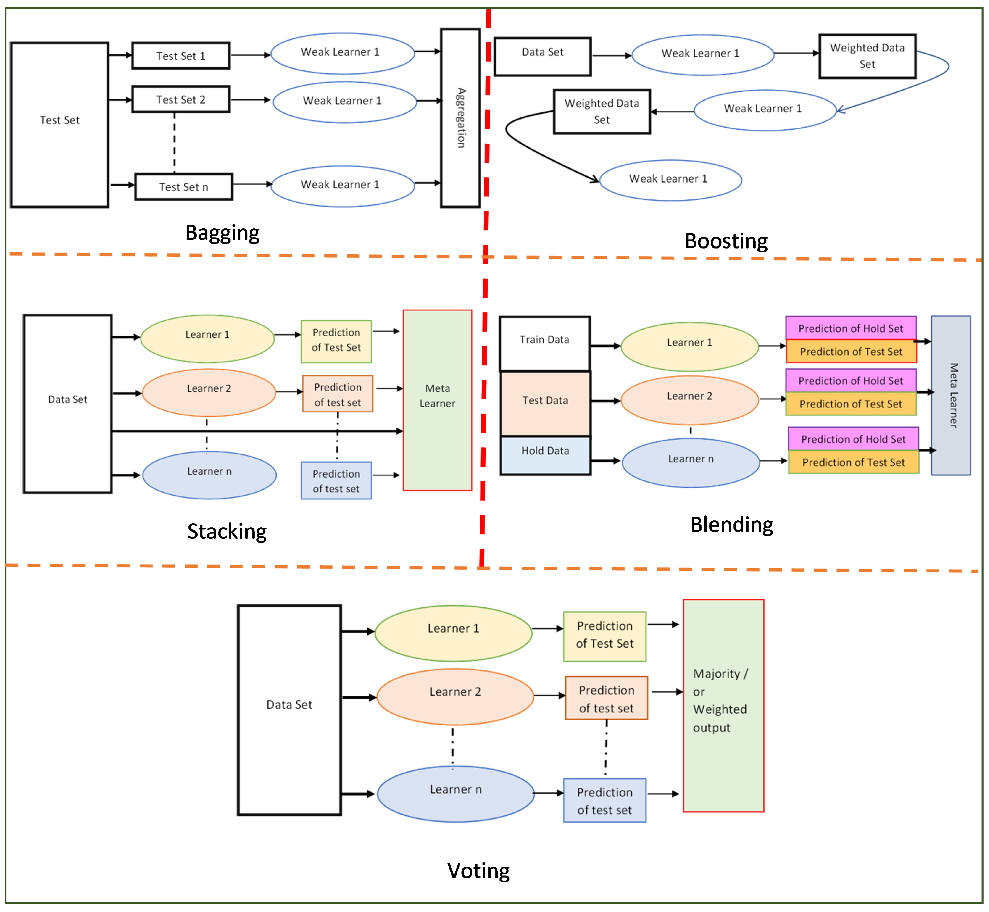
Ensemble Algorithms can be classified as Bagging, Boosting, Stacking, Blending, and Voting. The classification is based on whether the ensemble technique is sequential or parallel and whether the classifiers are homogenous or heterogeneous.
4.1. Bagging
In Bagging, the learning is done in parallel. The data set is classified into subsets, resampled (Boost-strapping) and fed to individual learners. All learners are of the same type and are weak learners. The output of these learners is then additively combined either by averaging or using the majority logic. The combination of Bootstrapping and Aggregation is Bagging. This is termed aggregation. The figure
Figure 1 depicts bagging, an example of which is Random Forest.
4.2. Boosting
4.2.1. Gradient Boosting
This is a stagewise addition method, where multiple weak learning algorithms are trained sequentially and a strong learner algorithm is used as a final model additively trained on multiple weak learning algorithms on the same dataset. It relies on the intuition that the best possible next model, when combined with previous models, minimizes the overall prediction error. The key idea is to set the target outcomes for this next model to minimize the error.
4.2.2. XGBoost (eXtreme Gradient Boosting)
This is a more regularized form of Gradient Boosting. XGBoost uses advanced regularization L1 (Lasso) and L2 (Ridge), which improve the model generalization capabilities. XGBoost delivers high performance as compared to Gradient Boosting. Its training is faster as it can be parallelized across clusters. The other gradient boosting methods, such as CAT Boost and LGM Boost, though faster than XGBoost are not used in our work as all our features are statistical, not categorical features.
4.2.3. ADABoost
Adaptive Boosting, is the most common estimator used with decision trees with one level which means Decision trees with only one split. These trees are also called Decision Stumps. This algorithm builds a model and gives equal weights to all the data points. It then uses the results to assign higher weights to points that are wrongly classified. Now all the points with higher weights are given more importance in the next model. It will keep training models until a lower error is received.
4.2.4. Stacking
In stacking, the learning is parallel, but the learners are heterogenous. The output of the learners is combined with the data set and fed to a meta-learner whose prediction is then taken as the final value.
4.2.5. Blending
With blending, instead of creating out-of-fold predictions for the train set, a small holdout set of say 10% of the train set is created. The stacker model then trains on this holdout set only. The meta-model trains and uses the prediction of the hold set and tests using the predictions of the test set.
4.2.6. Voting
Voting is an ensemble technique where multiple heterogeneous learners predict simultaneously and the prediction can be chosen using (a) Majority Logic, which is also termed as multiplicity. (b) Weights are assigned to each decision, and then a weighted output is compared against the threshold.
4.3. Algorithms Developed and used in this paper
4.3.1. Stack(A)
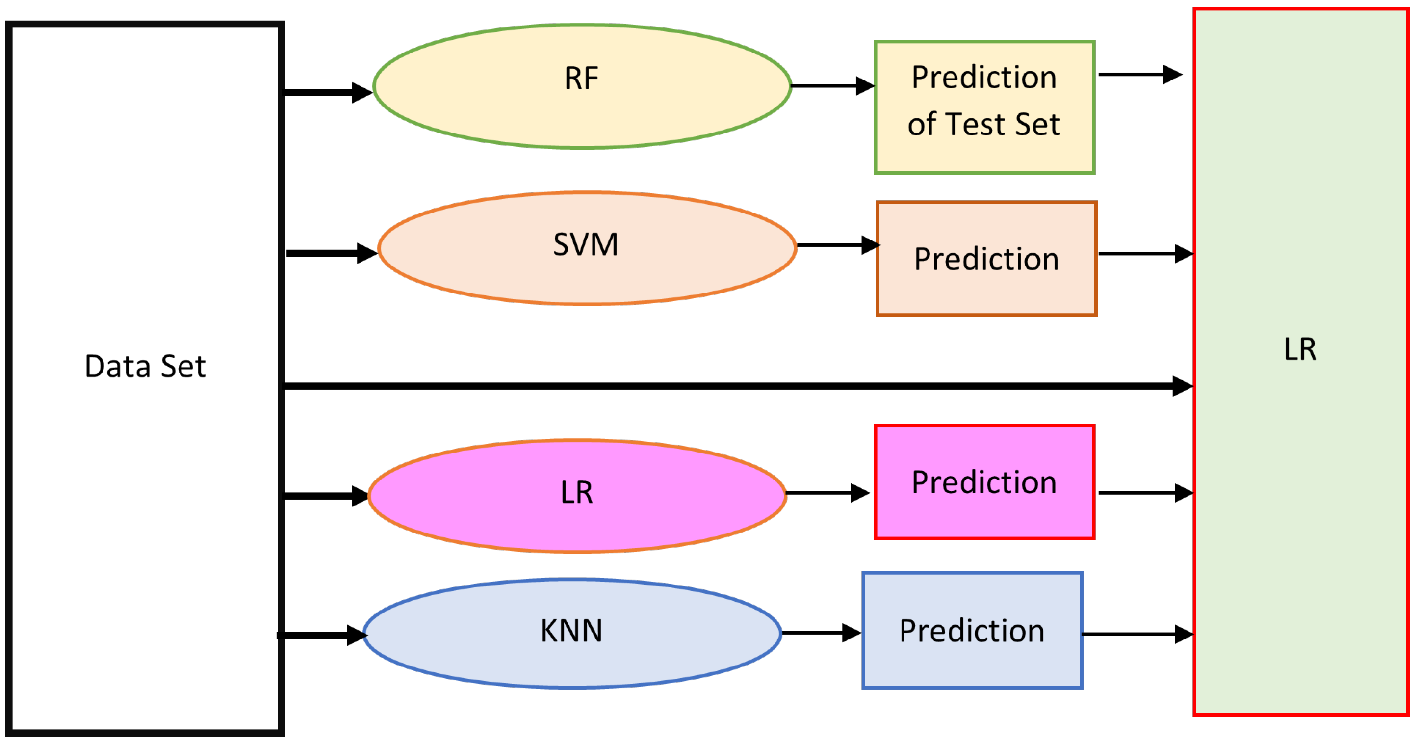
We tried various combinations of algorithms as first learners and meta learners (approximately 20 combinations) we got the best result as shown in
Figure 2
We got similar results when we used ADABoost, XGBoost, RF, and SVM but the latencies to run ADABoost is high hence we are using an ensemble of basic ML techniques that give the same type of accuracies but with less latency
4.3.2. VWE (B)
Voting-based Weighted Ensemble (B), uses heterogenous ensemble algorithms ADABoost, XGBoost, and Random Forest. We assigned varying weights to each of the ensemble’s predictions. The following equation was used:
We ran 500 different possible combinations of , & , we obtained the best accuracy results for .
4.3.3. VWE (C)
Voting-based Weighted Ensemble (C), uses heterogenous ensemble algorithms and non-ensemble algorithms SVM, XGBoost, and Random Forest. We assigned varying weights to each of the ensemble’s predictions. The following equation was used:
We ran 500 different possible combinations of , & , we obtained the best accuracy results for . Our voting methods are different in the sense that we do not use a simple majority but use a weighted value for every prediction.
5. Results and Discussion
5.1. Pruning
We initially ran all the ML algorithms with 112 features extracted. We analyzed the performance of all the algorithms (a) K-Nearest Neighbours (KNN) (b) Logistic Regression (LR) (c) SVM (Support Vector Machine). Each algorithm was run for 500 epochs. We ran for 500 epochs as that was where the accuracy and latency values started showing consistency.
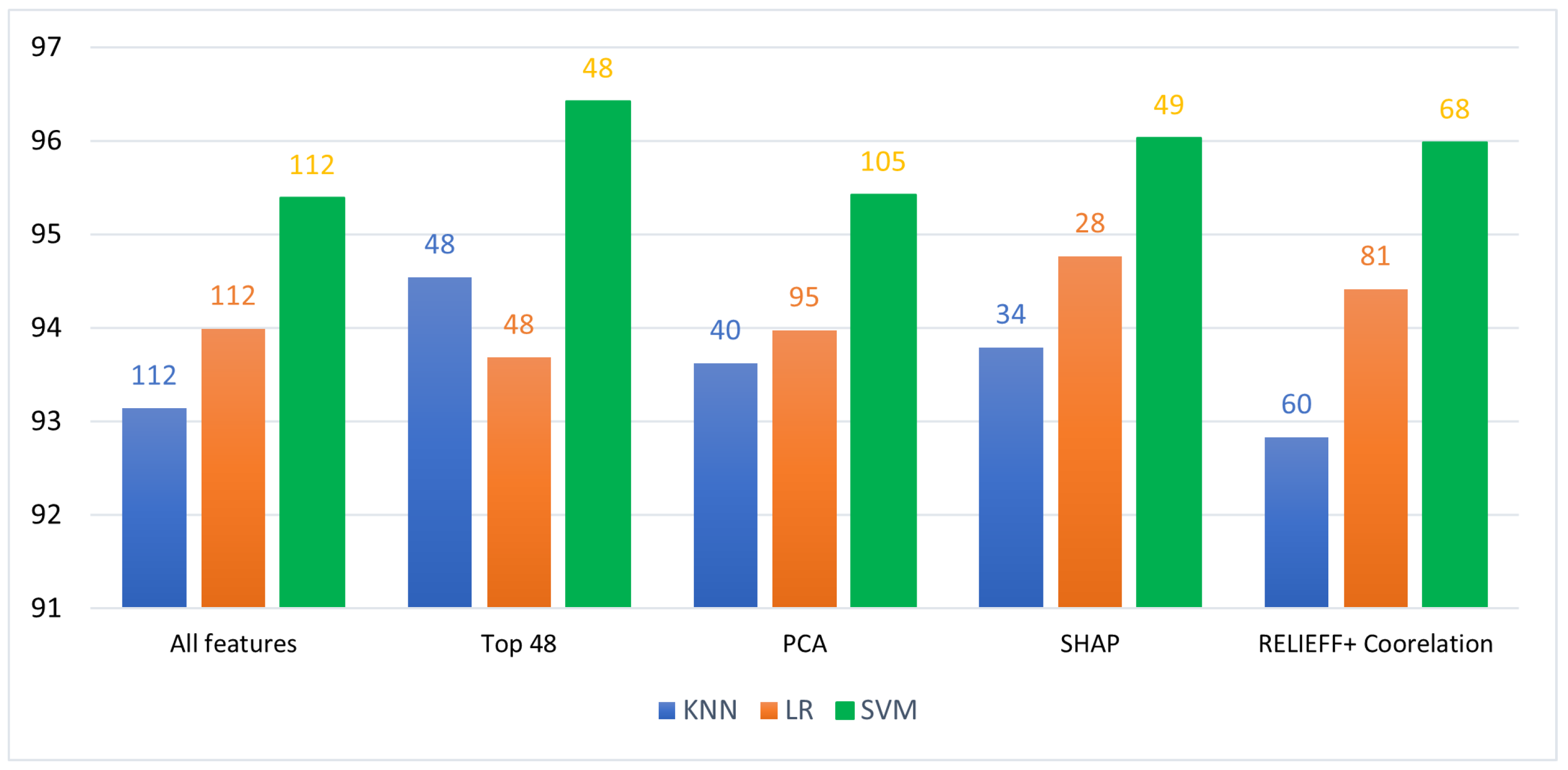
When all ML algorithms with all features were run the highest accuracy obtained was for SVM (95.3%). SVM classifies data by finding the best hyperplane that separates all data points of one class from those of the other class. The best hyperplane for an SVM means the one with the largest margin between the two classes.
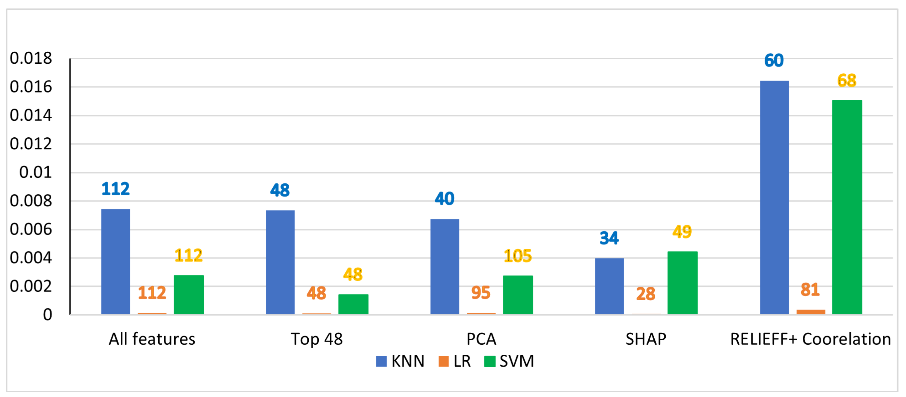
The latency was highest for KNN as we were using a K value of 9 (we got the highest accuracy when k was equal to 9 – we ran the KNN algorithm for K =3 to K = 91) KNN does run time training and testing as data comes in KNN makes a prediction by clustering with K neighbours hence high latencies can be expected. Logistic Regression gives the minimum latency irrespective of whether pruning was done or not. In the case of LR, a threshold comparison is done during train placing the prediction in the fall class or ADL class, and the time taken is proportional to the dimension of data, as our data dimension varied between 28 to 112. The time taken for LR varied accordingly. This is obvious when SHAP prunes the features to 28 as can be observed in
Figure 4.
To reduce the latency while retaining the accuracy we have to go in for feature pruning.
As described in section 3 we presented a brief overview of the pruning techniques. In this section, we present the results of applying the pruning techniques to the standard ML algorithms.
5.1.1. Column Drop
From
Figure 3 &
Figure 4 the accuracy and the latency we obtained can be observed. We analyzed the effect of individual statistical features on the accuracy. We are not presenting the results for all combinations as we tried with more than 500 combinations, but we got the best result for the top 3 statistical features for each data from the sensor. As we used 3-axis linear accelerometer, accelerometer, magnetometer, gyroscope, and heart rate. The number of features was a total of 48. This was obtained by taking the 3 axis of gyroscope, magnetometer and accelerometer, and the RMS values of the sensors were taken (this was 4*3 = 12 *3 = 36). The 3-axis values of the linear accelerometer without the RMS value were taken (3*3 = 9). The top 3 features of the heart rate sensor were taken. This gives a total of 36+9+ 3 = 48. The top three parameters were standard deviation, mean and minimum value.
There was a uniform increase in all algorithms especially in the case of SVM which gave an accuracy of 96.4%. The latency was decreased slightly as can be observed especially with Column Drop as they have the minimum number of features
5.1.2. Principal Component Analysis (PCA)
From
Figure 3 &
Figure 4 also gives the accuracy and latency when PCA is used as a pruning technique with ML algorithms.
As can be observed from the figures there is a slight increase in the accuracy of the ML algorithm, not much as in the case of column drop method but there is still an increase. The only algorithm that requires less than 48 features is KNN (40). The latencies again are higher in the case of KNN. This indicates more than the number of features; latency is determined by the complexity of the model under test.
We did not use PCA further as the increase in accuracy was less and PCA unlike other algorithms gives the top features fused and transformed into a new set of features and what those features were, is not available as an output from the algorithm. As we plan to use the features selected by each pruning method as the finalized features to run on the wristband SoC, this is not possible with PCA.
5.1.3. Shapley Pruning (SHAP)
Figure 3 &
Figure 4 give the accuracy & latency of Pruning using SHAP parameters. The improvement in accuracy when Shapley pruning is used is higher than that of PCA but slightly lesser than that of the column-drop method but the number of features required is less for all the ML algorithms except for SVM where the features selected are 49. Again, Latency is high for KNN and negligible for LR as the number of SHAP features is only 28.
LR takes the minimum latency also the accuracy is lower as logistic regression is more of a statistical method. It calculates the loss function a negative value that tries to reduce the error in predictions. This function is negative because when we train the model, we need to maximize the probability by minimizing the loss function. Decreasing the cost will increase the maximum likelihood, assuming that samples are drawn from an identically independent distribution. Hence LR works better with lesser features. It requires less training. It has good accuracy for many simple data sets, and it performs well when the dataset is linearly separable. Logistic regression is less inclined to over-fitting but it can overfit in high dimensional datasets. Hence LR works best with minimum features.
5.1.4. RELIEFF with cross-correlation
Initially, a cross-correlation threshold between features was applied. We obtained different thresholds per algorithm where the accuracy was high. The Correlation Thresholds were as follows:
KNN – 0.92
LR – 0.94
RF – 0.81
SVM- 0.91
The RELIEFF Feature Selection was run after removing features with high cross-correlation. The accuracy and the latency after pruning using RELIEFF are shown in
Figure 3 and
Figure 4.
The improvement in accuracy in RELIEFF is much lesser than SHAP or column drop methods. The number of features required is more than the other methods even after the features with high cross-correlation were removed. This is expected and has been computationally proved in [
27]. Again, SVM has the highest accuracy at 96% and requires 68 features.
The latency continues to be high in KNN, in this case, SVM also has high latency due to the increase in the number of features to 68 as compared to 48 or 49 in the earlier cases. Irrespective of which pruning method was used the accuracy has improved as using feature selection takes care of outliers and any overfitting.
5.2. Ensemble Algorithms with Pruning
We used six ensemble techniques – RF (Bagging), ADABoost and XGBoost (Boosting), and Stack (A) (stacking), VWE(B), VWE(C) (voting). We are not showing blending techniques as there was a huge drop in accuracy when blending was used irrespective of the pruning technique.
We first ran these algorithms on a CPU and then on Snapdragon 820c. The DragonBoard™ 820c development board is based on the Snapdragon® 820E embedded platform with a custom 64-bit Qualcomm® Kryo™ quad-core CPU and is compliant with the 96Boards Consumer Edition Extended Version specification managed by Linaro. The combination of the Snapdragon 820E embedded platform’s powerful Qualcomm® Adreno™ 530 GPU and quad-core CPU expands the possibilities of connected computing and high-power computing while consuming minimum power.
We have used the following pruning algorithms (a) Column Drop (b) Shapley (c) Correlation + RELIEFF We did not use PCA, since PCA does not give a set of features as output, but uses fused features and it does not list the fused features. Besides PCA showed very little improvement in accuracy after pruning.
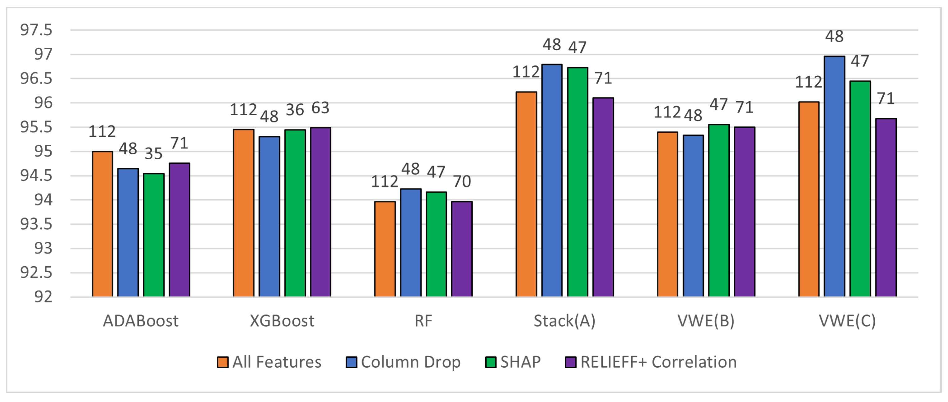
The variation in accuracy with the ensemble techniques is shown in the figure From
Figure 5 The best accuracies are obtained for Stack(A) at almost 97% for both Column Drop and SHAP methods. Column drop uses 48 features and SHAP 47 features. RELIEFF give slightly lower accuracies but is comparable with SHAP and Column drop. The only issue when using RELIEFF for pruning is the number of features is high at 71 also accuracy is lesser than when all 112 features are used. This eliminates RELIEFF as an ideal pruning technique. Column Drop is static whereas SHAP is dynamic irrespective of the data collected so the best pruning method.
SHAP and Column Drop gave similar results as 96% of the features selected by these pruning methods are the same.
VWE(C) gives good results in the case of column drop but there is a small drop of about 0.3% in the case of all pruning methods. In any case, VWE(B), the accuracies are higher than ADA and RF but lesser than XGBoost. VWEB has XGboost as one of its learners but ADABoost and RF who are the other learners seem to bring down the accuracy. We did vary the weightage of voting but this was the best accuracy obtained.
Among our three algorithms, the best performer is Stack(A). Even in the case of Stack(A) we tried various combinations of algorithms as the first learner and the meta-learner. We even tried less complex algorithms as the first learner( k-NN, LR, NB) and used SVM or ensemble algorithms as the meta-learner but are accuracies dropped to less than 93%. This is expected as the meta-learner learns from the first learners. If the first learners are strong the meta learner will be able to learn better.
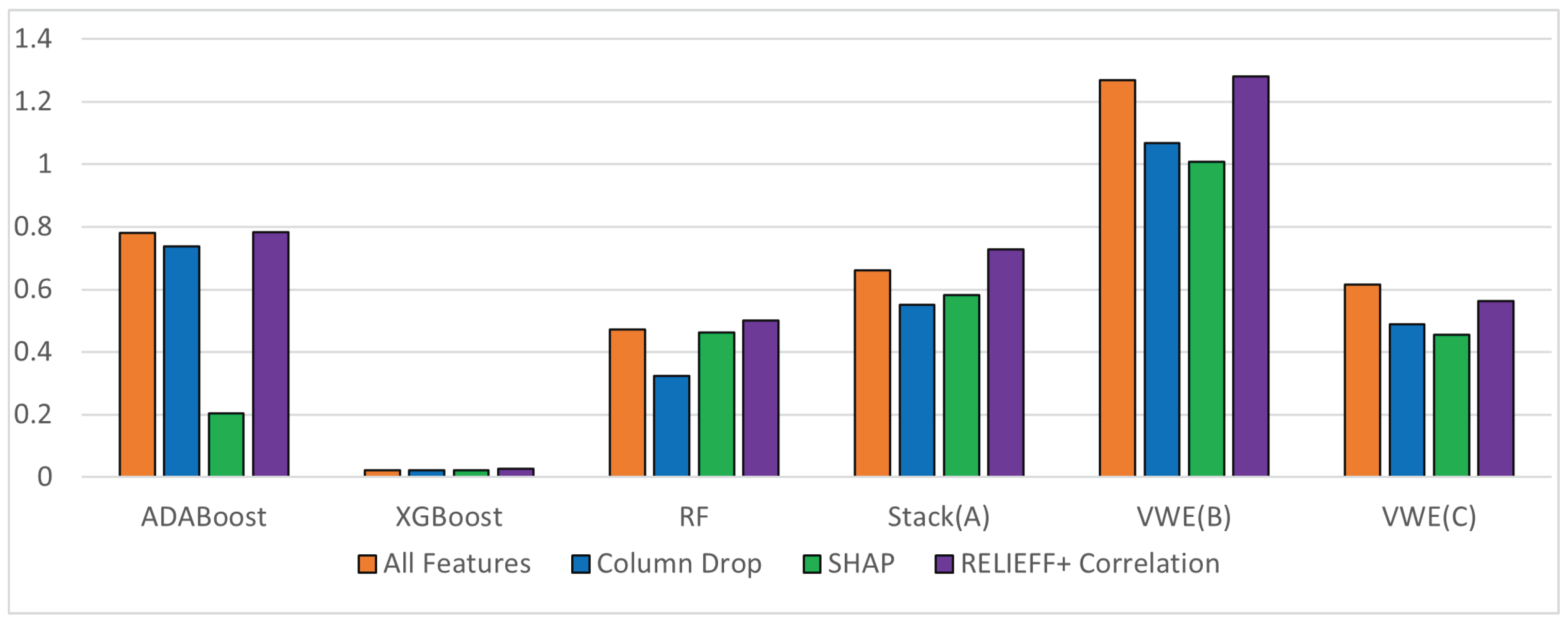
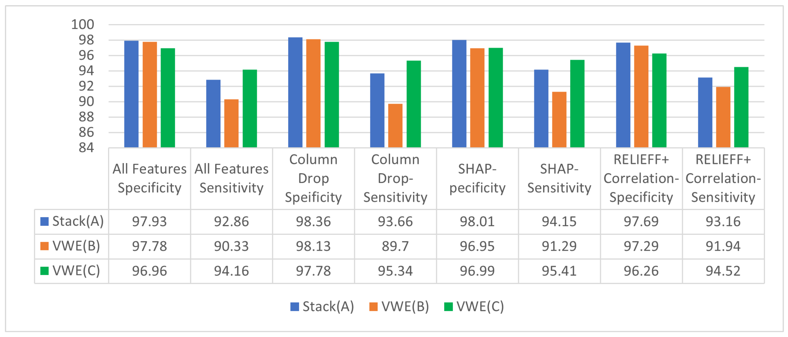
To understand the accuracies better we plotted the specificity and sensitivity. The specificity is high for all ensemble algorithms with all types of pruning. The specificity tells us when there is no fall. It minimizes false positives, contrary to the requirement that we do not want to miss any falls. Even if an ADL is misinterpreted as a fall it is better in our situation. The best sensitivities are obtained for VWE(C). Hence if sensitivity is important then VWE(C) is the better algorithm. Since our sensitivity is high, it means some of the ADLs are being incorrectly predicted as a fall. This is always better to err on the side of caution where the geriatric population is concerned.
Figure 7.
Latencies of ensemble algorithms with various pruning techniques.
Figure 7.
Latencies of ensemble algorithms with various pruning techniques.
In terms of latencies naturally XGBoost has the best latency but among our three algorithms, VWE(C) takes the minimum latency again for SHAP.
6. Summary
In this paper, we have presented three novel ensemble algorithms (a) Stack (A) (b) VWE(B) (c) VWE(C). The features that produced the maximum accuracy were used for training each ML algorithm. We collected IMU and heart rate data from 41 users. The features were extracted from the raw data. Generally, either feature extraction or selection is done. We initially extracted multiple statistical parameters from the raw data. Then different data pruning techniques were used to select the features for various ML algorithms. We have used the following pruning methods in this paper (a) Column Drop – where we use 48 features. (b)Principal Component Analysis (PCA). We did not use PCA further as in the case of PCA features are not identifiable, since PCA fuses features and do not produce a detailed output of the fused features. (c) SHAP (d) Cross-Correlation with RELIEFF.
We then ran the various ensemble algorithms (a) ADABoost (b) XGBoost (c) RF (d) Stack (A) (e) VWE(B) (f)VWE(C). The best accuracy was obtained for Stack(A) with SHAP as the pruning algorithm, Stack (A) also had higher specificity but low sensitivity. VWE(C) has slightly lesser accuracy but higher sensitivity which is a requirement of our application.
If the requirement is good specificity and accuracy the best algorithm is Stack(A) with SHAP for pruning. If we need good sensitivity at a slightly decreased accuracy, with low latency VWE(C) with SHAP for pruning is the best.
Our main aim in reducing the number of features is we want the ensemble algorithms to run on the end-device itself. Our end-device is built using Snapdragon 820c. Naturally, the accuracies remained the same on both the CPU and Snapdragon 820c. Even then The latencies on the Snapdragon with ensemble are higher than ML on the cloud. The latencies were less than milliseconds except where ADABoost was used so the ensemble algorithms with pruning can run on the end-device itself without any loss in accuracy or loss of data Since our data set had only 41 users in the feature, we plan to combine multiple data sets to train our ensemble with it. We then want to compare the performance against a DL technique such as RNN as our data is time series data. Also using wrist-based end-device make it very easy for the elderly to wear all through the day.
To summarize in this paper, we have combined feature extraction and selection both to trim the data so that the complexity and size of data is reduced and the algorithms even ensemble ones however complicated can be run on the end-device itself. We have proposed three different ensemble algorithms and presented scenarios where two of them (Stack(A), VWE(C)) would work better. The third algorithm (VWE(B)) is a combination of ensemble algorithms and will be used where the data set size is large and we need long-term analytics of the health data on the cloud. We can use VWE(B) for other geriatric health issues such as Sleep Apnea Detection or Lung based issues or Hiatal Hernia, all of which led to fatality among the geriatric population
References
- United Nations, D.o.E.; Social Affairs, W.P.A. World Population Ageing 2020 Highlights: Living arrangements of older persons, 2020.
- Anita Ramachandran, A.K. A Survey on Recent Advances in Wearable Fall Detection Systems. BioMed Research International, 2020; 17. [Google Scholar]
- Nandi, P.; Anupama, K.; Bajaj, A.; Shukla, S.; Musale, T.; Kachadiya, S. Performance evaluation of Machine Learning algorithms on System on Chips in Wearables for Healthcare Monitoring. Procedia Computer Science 2023, 218, 2755–2766. [Google Scholar] [CrossRef]
- Qualcomm. Snapdragon 820c Development Board, 2018. [Accessed 31-Mar-2023].
- Ray, P.P. An Introduction to Dew Computing: Definition, Concept and Implications. IEEE Access 2018, 6, 723–737. [Google Scholar] [CrossRef]
- Šojat, Z.; Skala, K. Views on the Role and Importance of Dew Computing in the Service and Control Technology. 2016. [CrossRef]
- Skala, K.; Šojat, Z. Cloud, Fog and Dew Computing: A Distributed Hierarchy. PhD thesis, 2015. [CrossRef]
- Vavoulas, G.; Pediaditis, M.; Chatzaki, C.; Spanakis, E.; Tsiknakis, M. The MobiFall Dataset:: Fall Detection and Classification with a Smartphone. International Journal of Monitoring and Surveillance Technologies Research 2016, 2, 44–56. [Google Scholar] [CrossRef]
- Sucerquia, A.; López, J.D.; Vargas-Bonilla, J.F. SisFall: A Fall and Movement Dataset. Sensors 2017, 17. [Google Scholar] [CrossRef] [PubMed]
- SmartFall Dataset, 2019.
- SmartWatch Dataset, 2018.
- Notch Dataset, 2016.
- Mauldin, T.; Canby, M.; Metsis, V.; Ngu, A.; Rivera, C. SmartFall: A Smartwatch-Based Fall Detection System Using Deep Learning. Sensors 2018, 18, 3363. [Google Scholar] [CrossRef]
- Nandi, P.; Anupama, K.; Agarwal, H.; Patel, K.; Bang, V.; Bharat, M.; Guru, M. Analysis of ML Algorithm for Geriatric Fall Detection Due to the Effects of Various User Characteristics. Preprints.org 2023 2023. [Google Scholar] [CrossRef]
- Escobar-Linero, E.; Luna-Perejón, F.; Muñoz-Saavedra, L.; Sevillano, J.L.; Domínguez-Morales, M. On the feature extraction process in machine learning. An experimental study about guided versus non-guided process in falling detection systems. Engineering Applications of Artificial Intelligence 2022, 114, 105170. [Google Scholar] [CrossRef]
- Venkatesh, B.; Anuradha, J. A Review of Feature Selection and Its Methods. Cybernetics and Information Technologies 2019, 19, 3–26. [Google Scholar] [CrossRef]
- Jolliffe, I.T.; Cadima, J. Principal component analysis: a review and recent developments. Philosophical Transactions of the Royal Society A: Mathematical, Physical and Engineering Sciences 2016, 374, 20150202. [Google Scholar] [CrossRef] [PubMed]
- Lundberg, S.M.; Lee, S.I. A unified approach to interpreting model predictions. Advances in neural information processing systems 2017, 30. [Google Scholar]
- Tripathi, S.; Hemachandra, N.; Trivedi, P. Interpretable feature subset selection: A Shapley value based approach. 2020 IEEE International Conference on Big Data (Big Data). IEEE, 2020, pp. 5463–5472.
- Gramegna, A.; Giudici, P. SHAP and LIME: An Evaluation of Discriminative Power in Credit Risk. Frontiers in Artificial Intelligence 2021, 4. [Google Scholar] [CrossRef] [PubMed]
- Chen, H.; Lundberg, S.M.; Lee, S.I. Explaining a series of models by propagating Shapley values. Nature Communications 2022, 13, 4512. [Google Scholar] [CrossRef] [PubMed]
- Ullah, I.; Rios, A.; Gala, V.; Mckeever, S. Explaining Deep Learning Models for Tabular Data Using Layer-Wise Relevance Propagation. Applied Sciences 2022, 12. [Google Scholar] [CrossRef]
- Kononenko, I.; Šimec, E.; Robnik-Šikonja, M. Overcoming the Myopia of Inductive Learning Algorithms with RELIEFF. Applied Intelligence 1997, 7, 39–55. [Google Scholar] [CrossRef]
- Urbanowicz, R.J.; Meeker, M.; La Cava, W.; Olson, R.S.; Moore, J.H. Relief-based feature selection: Introduction and review. Journal of Biomedical Informatics 2018, 85, 189–203. [Google Scholar] [CrossRef] [PubMed]
- Zhang, Y.; Song, X.f.; Gong, D.w. A return-cost-based binary firefly algorithm for feature selection. Information Sciences 2017, 418, 561–574. [Google Scholar] [CrossRef]
- Le, T.T.; Urbanowicz, R.J.; Moore, J.H.; McKinney, B.A. STatistical Inference Relief (STIR) feature selection. Bioinformatics 2018, 35, 1358–1365. [Google Scholar] [CrossRef] [PubMed]
- Tripathi, S.; Hemachandra, N.; Trivedi, P. Interpretable feature subset selection: A Shapley value based approach. 2020 IEEE International Conference on Big Data (Big Data), 2020, pp. 5463–5472. [CrossRef]
|
Disclaimer/Publisher’s Note: The statements, opinions and data contained in all publications are solely those of the individual author(s) and contributor(s) and not of MDPI and/or the editor(s). MDPI and/or the editor(s) disclaim responsibility for any injury to people or property resulting from any ideas, methods, instructions or products referred to in the content. |
© 2020 by the authors. Licensee MDPI, Basel, Switzerland. This article is an open access article distributed under the terms and conditions of the Creative Commons Attribution (CC BY) license (https://creativecommons.org/licenses/by/4.0/).
