Preprint
Article

Fish Monitoring from Low Contrast Underwater Images

Altmetrics

Downloads

144

Views

61

Comments

0

A peer-reviewed article of this preprint also exists.

Submitted:

12 June 2023

Posted:

12 June 2023

You are already at the latest version

Alerts
Abstract
A morphological feature estimation method is presented, that can be used to monitor fish from low contrast underwater images and videos. The fish orientation is classified in order to apply a shape alignment technique that is based on the Ensemble of Regression Trees machine learning method. Shape alignment allows the estimation of fish dimensions (length, height, mass) and the location of fish body parts of particular interest such as the eyes and gills. The developed system can be exploited both for fish monitoring in open sea as well as aquacultures where non-invasive, low cost morphological feature extraction is essential. Fish health can be assessed from malformations in body shape, the color of the eyes or the gills as well as the fish behavior. The proposed method can estimate the position of 18 landmarks with an accuracy of about 95% from low resolution and low contrast underwater images where the fish can be hardly distinguished from its background. Hardware acceleration can be applied at various stages of the proposed method for real time video processing. As a case study, the developed system has been trained and tested with several Mediterranean fish species in the category of seabream or similar: diplodous sargus annularis (white seabream), diplodus annularis seabream (spawn), oblada melanura (saddled seabream), pagrus pagrus (common seabream), etc. A large dataset with low resolution underwater videos and images has been created in the context of this work.
Keywords: 
Subject: Computer Science and Mathematics  -   Artificial Intelligence and Machine Learning

1. Introduction

Measuring fish morphological features and observing their behavior are important tasks that have to be carried out daily, in fish cultures. The morphological features include the body dimensions, estimation of the fish mass, eye diameter and color, the gill color as well as malformations in their shape. These features can be used to assess the welfare of the fish, growing conditions, their health and feeding needs. The behavior of the fish can be characterized by its trajectory, its speed, etc, and is an important indication of stress, starvation and health status. These indications are taken into consideration in fish farms to optimize the feeding process, stock control and the proper time for harvest. The measurement of fish dimensions, weight, etc, was performed manually until recently, in an invasive way, by taking sample fish out of the water. This is a manual, time consuming, high cost, inaccurate and harmful for the fish, procedure. Tasks like fish tracking and classification, morphological feature estimation and behavior monitoring are also important in observing the population of various species in rivers or the open sea.
A review of smart aquaculture systems has been presented in [1] where several processes are described for breeding, nursery to grow out stages of cultured species, preparation of cultured water resource, management of water quality, feed preparation, counting, washing the cultured systems, etc. Another review of computer vision applications for aquaculture is presented in [2]. These applications include fish and egg counting, size measurement, mass estimation, gender detection, quality inspection, species and stock identification, monitoring of welfare and behavior. The trends in the application of imaging technologies for the inspection of fish products are examined in [3]. The reviewed image processing approaches are classified by the position of the light source (reflectance, transillumination, transflectance, etc). The applications examined include rigor mortis, tissue and skin color as well as morphology to determine fat, firmness, shape, wounds, blood detection, etc.
Several approaches have been proposed concerning the estimation of fish freshness in a controlled lab environment, based either on sensors or image processing. In [4], various sensors that have been used in the literature for freshness estimation are reviewed. These sensors include biosensors, electric nose or tongue, colorimetric sensor array, dielectric and various sensor for spectroscopy (nuclear magnetic resonance, Raman, optical, near infrared, fluorescence, etc). Quality management systems have also been proposed for freshness, safety, traceability of products, adopted processes, diseases and authenticity [5]. In [6], the freshness of Scomber japonicus (mackerel) stored at a low temperature is assessed from the correlations between the light reflection intensity of mackerel eyes and the volatile basic nitrogen content. The assessment of fish freshness from the color of the eyes is also examined in [7]. In this approach, a handheld Raspberry PI device is used to classify the freshness of a fish in three categories (extremely fresh, fresh, spoiled) based on pixel counting.
Fish classification and counting from underwater images and videos is another major category where several approaches have been proposed in the literature. In [8], fish appearing in underwater images are classified in 12 classes based on Fast Regional-Convolutional Neural Networks (Fast R-CNNs). Similarly, in [9], You-Only-Look-Once (YOLO) [10] and Gaussian Mixture Models (GMM) [11] are compared for the classification of 15 species with an accuracy between 40% and 100% (>80% in most cases). Lekunberri et al [12], count and classify various tuna fish species transferred on conveyor belt with 70% accuracy. Their approach is based on various types of neural networks (Mask R-CNN [13], ResNet50V2 [14]) while the size of tuna fish, ranging from 23cm to 62cm, is also measured. Underwater fish recognition is performed in [15] with an accuracy of 98.64%. Similarly, fish recognition from low resolution images is performed in [16] with 78% precision.
Morphological feature estimation is often based on active and passive 3D reconstruction techniques. The active techniques are more accurate but require expensive equipment such as Lidars, while passive technique employ lower cost cameras. Challenges of passive 3D reconstruction include the accurate depth estimation from two images that have been retrieved concurrently, occlusions, patterns and saturate areas that may cause confusion. In [17] a system based on stereo camera is described for accurate fish length estimation as well as fish tracking. A monocular 3D fish reconstruction is presented in [18] where successive images are used from fish carried on a conveyor belt in order to measure their size. CNNs implemented on Graphical Processing Units (GPUs) are used for foreground segmentation and stereo matching. A median accuracy of less than 5mm can be achieved using an equivalent baseline of 62mm.
In [19], Facebook’s Detectron2 machine learning (ML) library has been employed for object detection and image preprocessing to generate 22 metadata properties including morphological features of the examined specimens with error rates as low as 1.1%. Otsu threshold is used for segmentation of relatively simple images and pattern matching to locate the eye. If the fish is detected without eye the images are upscaled.
Fish tracking (and classification) can be performed with both optical and sonar imaging as described in [20]. Using sonar imaging is the only way to monitor fish in night time. In this approach, the Norfair [21] tracking algorithm in combination with YOLOv4 [22] are used to track and count fish. The employed sonar equipment, is dual-frequency identification sonar (DIDSON) that exploits higher frequencies and more sub-beams than common hydroacoustic tools. The use of DIDSON has also been described in [23] for the detection of fish morphology and swimming behavior. In this approach, fish must be large enough and in an adequate distance thus, it is not appropriate for counting small fish. Fish length should preferably be around 68 cm, otherwise an estimation error ranging from 2%-8% was measured for fish with different size (40cm–90cm). In [24], optical and sonar images are also employed for fish monitoring.
In the system described in this paper, a three-stage approach is followed to detect fish in low quality image frames where fish cannot be easily discriminated from the background. The input image frame is segmented to extract the bounding boxes of the detected fish as separate image patches. In the second stage, each patch is classified to a draft orientation in order to select the corresponding pre-trained ML model that can align a number of landmarks on the fish body. The shape (and potential malformations) of the fish can be recognized in the third stage in order to measure fish dimensions, to classify fish in categories and to map fish body parts of special interest such as the eyes and gill.
In the first stage of the proposed system, the open source, fish detection, deep learning method presented in [25] was employed. Although detailed instructions are given on how to train a customized fish detection model, the pre-trained one performed very well even with the low resolution images of the developed dataset. Therefore, the pre-trained model was stored on the target platform and was called from an appropriate Python script that was developed for image segmentation. The output of this script is a number of image patches, and each one of these patches contains a single fish. The coordinates of these patches in the original input frame are also extracted. Each one of the image patches is classified in a draft fish orientation category following high speed methods, based on OpenCV [26] services. The coordinates of the patches can be used to track the movement of the fish in successive frames. The short history of fish positions that have been detected in the first stage can be used to estimate extended bounding boxes for the intermediate positions through interpolation in order to bypass the time consuming fish detection process in some frames.
The extracted patches from each image frame are used as inputs to the last stage of the developed system that performs shape alignment. Aligning a number of landmarks is based on the machine learning (ML) approach called Ensemble of Regression Trees (ERT) presented by Kazemi and Sullivan in [27] and is exploited in popular image processing libraries such as DLIB [28] and Deformable Shape Tracking (DEST) [29]. The DEST library has been exploited in our previous work [30] for driver drowsiness applications. The source code of the DEST library was ported to Ubuntu and Xilinx Vitis environments to support hardware acceleration of the shape alignment process on embedded targets. The DEST library has also been ported to MS Visual Studio 2019 environment and this version is adapted in this work for fish shape alignment.
Previous work on fish morphological feature measurement has also been presented by one of the authors in [31] but it concerned different fish species and employed different approaches for image segmentation, pattern matching and contour recognition. The fish contour detection method followed in [31] were not based on shape alignment and ERT. However, the absolute fish dimension estimation with stereo vision presented in [31] is also applicable in this work too.
The contribution of the present work can be summarized in the following: a) shape alignment based on ERT models is employed for high precision morphological feature estimation, b) different ERT models are trained for different fish orientations, c) high speed fish orientation detection is performed based on OpenCV services, d) an accurate fish detection method capable of detecting fish in low resolution images is adopted, e) fish tracking is supported and f) hardware acceleration techniques are applicable at the fish detection and shape alignment stages for real time video processing.
This paper is organized as follows. The materials and methods used, are described in Section 2. More specifically, the dataset, tools and target environment are presented in 2.1. The general architecture of the proposed system is described in 2.2. The employed fish detection and the fish orientation methods are described in 2.3 and 2.4, respectively. The methodology for implementing fish tracking is described in 2.5. The ERT background and the customized DEST package used for fish shape alignment and morphological feature extraction are described in 2.6 and 2.7, respectively. The experimental results are presented in Section 3. A discussion on the experimental results, follows in Section 4 and the conclusions are presented in Section 5.

2. Materials and Methods

2.1. Dataset, Tools and Target Environment

The image datasets used in similar fish monitoring applications usually consist either of images that have been captured in a lab environment under controlled light exposure, or high resolution underwater images where the fish are clearly visible. The images and videos used in the context of this paper have been retrieved using a low cost camera (TurboX Act201), their image resolution is 4608 × 3456 and the video resolution is 3840 × 2160, with a frame rate equal to 30 frames per second (fps). The photographs and videos of the developed dataset have been captured in two regions in Greece (Lampiri, Achaia and Gavathas, Lesvos island) and display Mediterranean fish species mostly seabream variations such as diplodous sargus annularis (white seabream), diplodus annularis seabream (spawn), oblada melanura (saddled seabream), pagrus pagrus (common seabream), etc. The trained ERT model aligns 18 landmarks on the fish body and can also be used with other species that have similar shape and color such as sithognathus mormyrus, sparus aurata, dicentrarchus labrax, etc. New ERT models can be easily retrained for different number of landmarks and fish shapes. The images/videos of the developed dataset have been captured both in sunny and cloudy days with calm or stormy sea. The images have been captured close to sea level and display fish in a depth between 0.5 and 3 meters.
From the initial large selection of videos and photographs, a relatively small number of image frames (400) have been used to generate 300 single fish image patches. The fish in these patches has a specific orientation e.g., horizontal body-facing left, or with tilt facing up-right, etc. An example photograph and a video frame with the corresponding fish patches extracted, are shown in Figure 1. As can be seen from Figure 1, the fish in these image frames, are hardly distinguishable from their background. Consequently, the fish detection, monitoring and morphological feature extraction methods presented in this paper are applied in worst case conditions.
The host computer used in the experiments is an ordinary Dell laptop with Intel(R) Core(TM) i5-1035G1 CPU @ 1.00GHz and 16GB RAM. The artificial intelligence (AI) inference for fish detection, the orientation classification script and the training/testing of the ERT model for shape alignment were installed on this computer. As will be discussed in subsection 2.7, the target board can be an embedded platform such as a Xilinx ZCU102 with ZynqMP Ultrascale+ field programmable gate array (FPGA) in order to support hardware acceleration and real time video processing. Concerning the programming languages used for the development of the system presented in this paper, the fish detection and orientation scripts are implemented in Python while the shape alignment is implemented in C++ (Visual Studio 2019 environment). A new landmark annotation editor (LAE) has also been developed in Visual Studio 2019, in C# as a Universal Windows Program (UWP) and is presented in subsection 2.7

2.2. General Architecture of the Proposed System

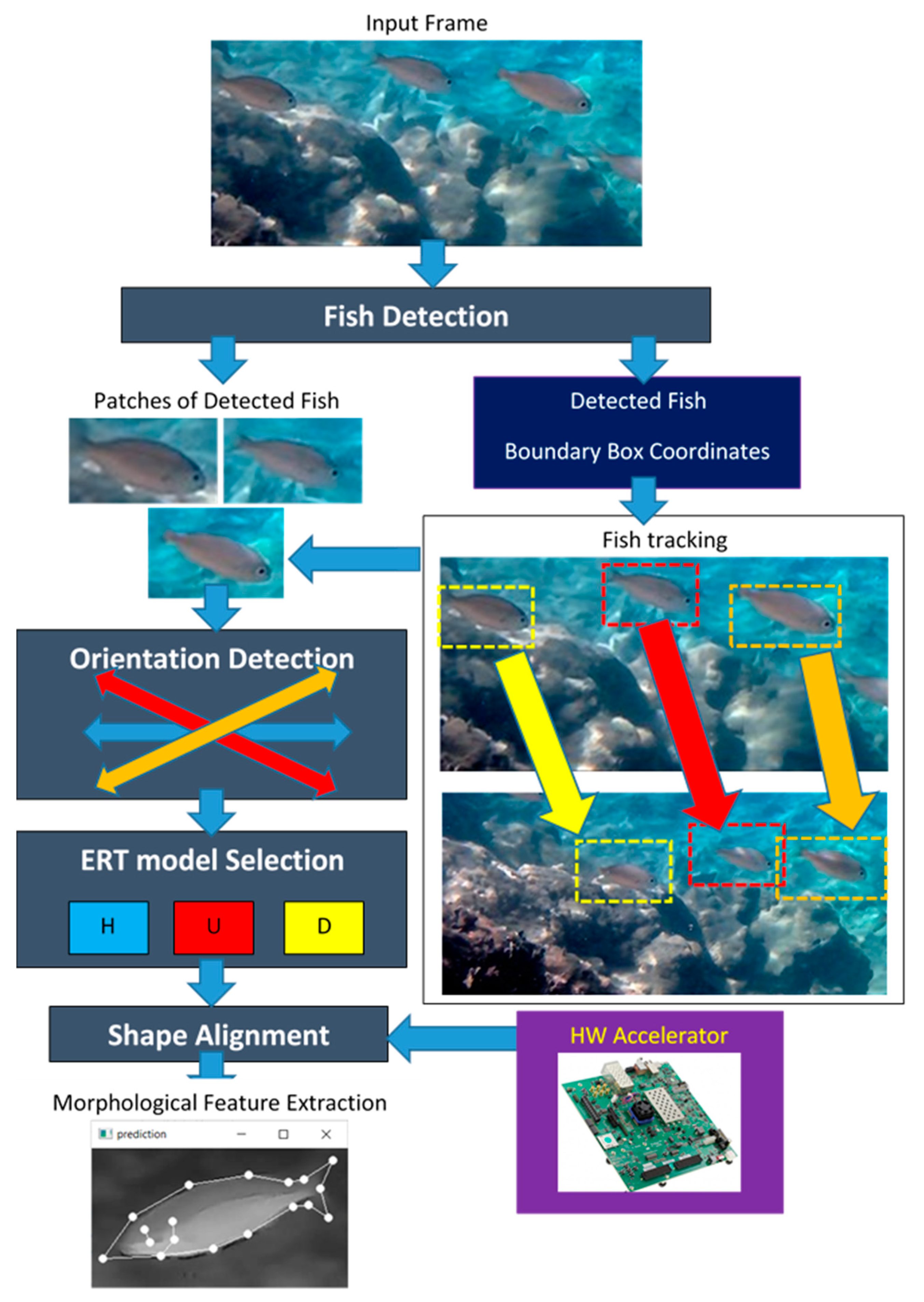
The architecture of the proposed fish monitoring and morphological feature estimation system is shown in Figure 2. The input of the system is either a single photograph or a frame from an input video stream. A customized Python script based on the open source code and the pre-trained fish detection model presented in [25], analyzes the input image frame and detects the bounding boxes of the fish. The coordinates of these bounding boxes are used to crop patches displaying a single fish. These patches are used as input to the next stage that detects fish orientation. The orientation of the fish is necessary in order to select the appropriate pre-trained ERT model for shape alignment. The ERT ML method employed for shape alignment is based on the correction of a mean shape stored in the pre-trained model. This correction procedure cannot support a rotation in the mean shape by more than ±20o. For this reason, different ERT models are trained for each direction and the appropriate model is selected by the orientation classification module for the shape alignment process.
The output of shape alignment stage is the set of 18 landmark coordinates that determine the location of fish body parts of particular interest such as the mouth, the eyes, the caudal fin, etc. From the distance of these landmarks, fish morphological features such as the relative fish length/height and its shape can be extracted. The shape alignment process can be accelerated with the aid of an embedded hardware platform as described in [30].
The AI inference of the model used for fish detection can also be accelerated in hardware since it is a time consuming process. However, an alternative way based on interpolation can be followed to speed up the fish detection process without special hardware support. Its aim is to define extended bounding boxes in the frames where fish detection is not applied for faster operation. If the shape alignment performed in one of the interpolated bounding boxes fails then, the results based on the extended bounding box approximation are invalidated. A small image frame buffering (e.g., of 10 image frames) is necessary to guarantee that all the processing results are correct. The successive positions of a fish are registered to track its movement in order to study its behavior.

2.3. Employed Fish Detection Approach

The fish detection method employed in this paper, is based on the tools presented in [25]. With this repository, the developer has the option either to use a pre-trained model or customize a new model, following the instructions given. The training process can be performed in an Ubuntu environment using a docker and consists in short of the following steps: a) a tensor flow object detection github repository is cloned, b) the training dataset has to be prepared in tfrecord format, c) a new label map should be created, d) an existing model like Faster RCNN has to be downloaded, e) a copy of an appropriate configuration has to be created and customized, f) the model should be trained using an available Python script, g) the validation results can be observed, h) a graph in .pb format has to be extracted and used as inference, i) the inference can be called within a Jupyter notebook or in Collab environment. The creator of the repository in [25] also offers a pre-trained .pb model as the one that can be generated in step (h). This model proved extremely sensitive for our dataset and even fish that were hardly recognized with the naked eye, have been detected by this model.
Certain Python scripts offered in [25], have to be executed when the fishes in a new image frame have to be recognized. The modification of these Python scripts was necessary in order to run the inference locally, i.e., outside a Jupyter environment and integrate the fish detection process in our flow. The coordinates of the bounding box of a detected fish are used to crop the initial image and generate a patch that will be used in the orientation detection and the shape alignment stages of the developed system. The bounding box coordinates are also passed to the fish tracking stage. Figure 1a shows the detection of 3 fish from an input photograph and Figure 1b, the detection of 2 fish from a video frame.
The drawback of this fish detection approach is the large latency required for the analysis of a single image. After loading the inference model, the Python script that performs the inference needs about 1.6 seconds to analyze each video frame, on an Intel i5, 1GHz processor and about Lfd=1 second on an Intel Core i5-9500 CPU @3.00GHz, 6 core processor with 16GB RAM. Video processing in real time would not be possible if fish detection had to be applied to all the input frames. One approach would be to accelerate the inference on a GPU or an embedded hardware platform. Lightweight or pruned NN models can also be trained following the procedure described in [25] to achieve higher speed with a slightly lower accuracy. Another lower cost approach is to buffer the video frames, apply fish detection in regular time intervals and interpolate the position of the fish between successive fish detections. This method will be examined in more detail and will be called henceforth: Fish Position Interpolation (FPI).
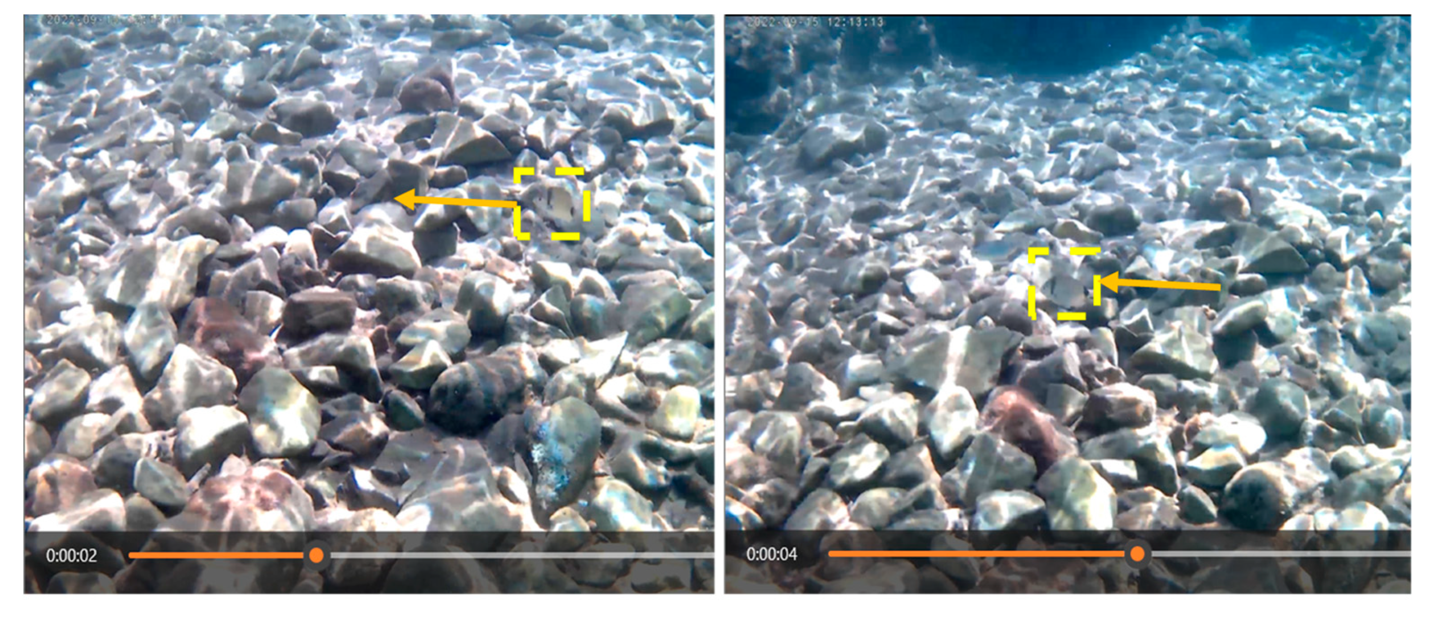
In FPI, it will be assumed that fish detection takes place every Tfd seconds. In modern multi-core processors Tfd can be as low as Lfd, since one thread can run the inference and another parallel thread can run the FPI between successive fish detections that took place with a time distance of Tfd. The fish orientation between successive fish detections does not necessarily have to remain the same, since the orientation detection may also be applied to the interpolated bounding boxes. However, if fish is found to have the same draft orientation between successive fish detections, the orientation detection procedure does not need to be repeated in the interpolated positions to speed up the whole process. For example, as can be seen in Figure 3, a fish is moving in the same direction (denoted by the orange arrow) for 2 seconds.
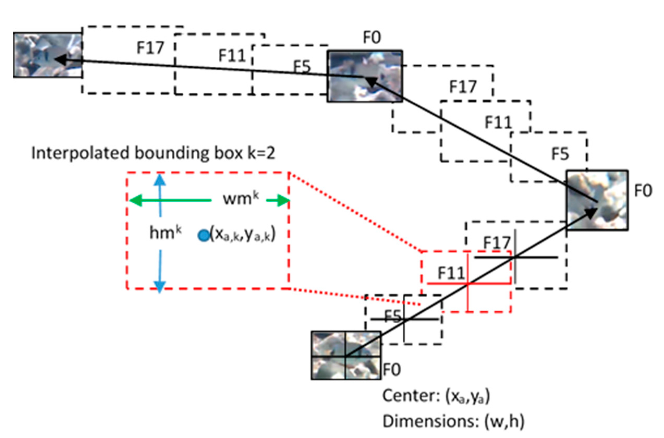
The FPI procedure is described in more detail in Figure 4. If the input stream has a standard frame processing speed of 24 fps, it is assumed that shape alignment is adequate to be applied every 6 frames, i.e., every 0.25sec. More intermediate shape alignments may be applied in shorter intervals but they are not expected to give more information about the track, the behavior and the morphological features of a fish. Thus, if a fish detection takes place every Tfd=1sec, at frame No. 0 (F0), the bounding boxes of the fish in frames No. 5 (F5), 11 (F11) and 17 (F17) have to be interpolated. For this purpose, the center of the 1st bounding box (F0) and the center of the bounding box generated from the next fish detection are located. The straight line connecting these bounding box centers is split according to the number of interpolations If that will be performed. As shown in Figure 4, the distance between two successive fish detections is split in 4 equal segments in order to define the center of the If interpolated frames (F5, F11 and F17). The size of the interpolated bounding boxes is incremented by a fraction z. The value of z was experimentally selected between 10% and 20%. Obviously, if z=20% is selected, the dimensions of F17 will be 172.8% larger than the original bounding box. If the size of the bounding box gets too large compared to the fish dimensions displayed in this box, the shape alignment accuracy will be degraded. On the other hand, if z=10%, F17 dimensions will be only 133.1% larger than the original bounding box. The shape alignment accuracy in this case would be higher but with a higher risk to get an interpolated bounding box where parts of the fish will be excluded, or even a bounding box that does not display a fish at all.
The general formal definition of the interpolation between two successive fish detection bounding boxes with centers (xa, ya) and (xb, yb) follows. If If interpolation bounding boxes are defined, the center (xa,k, ya,k) of the k-th (0<k≤If) interpolation bounding box is defined as:
x a , j , y a , j = ( x a + k x b x a I f + 1 , y a + k y b y a I f + 1 )
If the width and the height of the original bounding box is wbb and hbb, respectively, then, the corresponding dimensions wbb,k and hbb,k are defined as:
w b b , k , h b b , k = ( w b b · z k , h b b · z k )

2.4. Orientation Classification Method

The ERT model [27] that will be used for the shape alignment and consequently for the measurement of the morphological features of the fish has to be trained on fish that have similar orientation. The human face shape alignment approach presented in [27] and widely used in popular libraries like DLIB [28], defines the facial shape with 68 landmarks and is more tolerant on the tilt of the head due to the symmetry of the shape. The face shape is symmetrical since every landmark has a horizontal mirror landmark. This fact is actually exploited when training an ERT model, since the training dataset is augmented with the mirror images. The 2D shape of the fish side view is the most important since besides the length and height of the fish that can be estimated, special Regions of Interest (ROIs) can also be located in the fish body. Such ROIs are the eyes and the gills since the health of the fish can be assessed from the color of these regions. Moreover, fish shape malformations can be detected from the side view. The employed ERT ML method for shape alignment is tolerant to a tilt of the shape of about 20o.
An option would be to detect the 1D orientation of the fish on the image plane and rotate or mirror it before performing shape alignment. Horizontal mirroring is actually an applicable operation that does not affect the achieved accuracy i.e., a model trained with fish facing left are expected to have the same accuracy with a model trained with fish facing right. However, in the general case, a fish with tilt higher than 20o, may not have exactly the same shape with a fish captured horizontally, as shown in Figure 5 (depending also on the camera view of angle). For this reason, different ERT models have to be trained for a small number of distinct orientations in order to achieve an accurate shape alignment. Even if we are interested only in images with fish in horizontal position, it is necessary to detect the draft orientation in order to reject images where the fish is not horizontal or use them merely for fish tracking and not morphological feature extraction.
Concerning the approaches presented in the literature for object orientation, 1D orientation of vehicles is achieved in [32] based on a YOLO network architecture with a modified output fully connected layer (enriched with additional orientation parameters). Deep CNNs (DCNNs) are used in [33] for a continuous object orientation estimation between 0 and 360 degrees. Three continuous orientation prediction approaches based on DCNNs are described in [33]. In the first two, the orientation is represented as a point on a unit circle and either L2 loss or angular difference loss is minimized. In the third more efficient method, the continuous orientation estimation task is transformed into a set of discrete orientation estimations (as also required in our case) and then, the discrete orientation is converted to a continuous one with a mean-shift algorithm.
Principal Component Analysis (PCA) has also been proposed for feature extraction of a dataset. PCA accepts as input all the features of a dataset, but only considers a subset of features that are important to detect correlations between the selected features, resulting in a reduced dimensionality of the dataset [34]. The eigenvectors presented in the PCA process are determining the directions along which, the data have the highest variance [35]. In [36], OpenCV services are used to determine the direction of objects in images that are well discriminated.
A brief introduction to the PCA process follows. Let’s suppose we have a matrix Xrxn=[X1 X2 … Xn] with measurements. Xi is a sub-vector of r elements sj, which is necessary for the calculation of principal components. The covariance matrix with each Xi needs to be calculated for the measurement of the variability or spread in the dataset.
R r × r = i = 1 r X i X i T
The singular value decomposition (SVD) of (R)rxr, is defined as follows:
( R ) r × r = U S d V T
Sd is a diagonal matrix with the singular values of R on its diagonal, while V is a matrix having the right singular vectors of R as columns. U=[U1 U2 … Un] is a feature vector (matrix of vectors). The columns of U are the left singular vectors of R.
The first m sub-vectors from the vector U are preserved while the rest are discarded. In other words, the first m eigenvectors (ordered by magnitude) are used in order to create (Ureduced )nxm =[U1 U2 … Um], m<n. Those elements correspond to the principal components that can be used as a compressed version of the original input. More specifically, the transpose of the vector (Ureduced)nxm can be multiplied with the original data set:
( Y i ) m × 1 = ( U r e d u c e d T ) m × n ( X i ) n × 1
The original data can be restored with the following equation:
( X i r e c e i v e d ) n × 1 = ( U r e d u c e d ) n × m ( Y i ) m × 1
The detection of the draft fish orientation in our approach has to be performed with high speed and thus, DL methods are not appropriate due to their high latency. OpenCV PCA and image segmentation methods can offer an alternative faster solution with good accuracy. More specifically, the PCA method described in [36] has been adapted in our framework. In 95% of the cases the tilt of the fish is detected accurately in the patches extracted by the fish detection stage. However, only in 45% of the cases, the detection of the direction the fish is facing at, was correct. The employed PCA method, converts the input image patch in grayscale and resizes it. All resized patches have 320 pixels height.
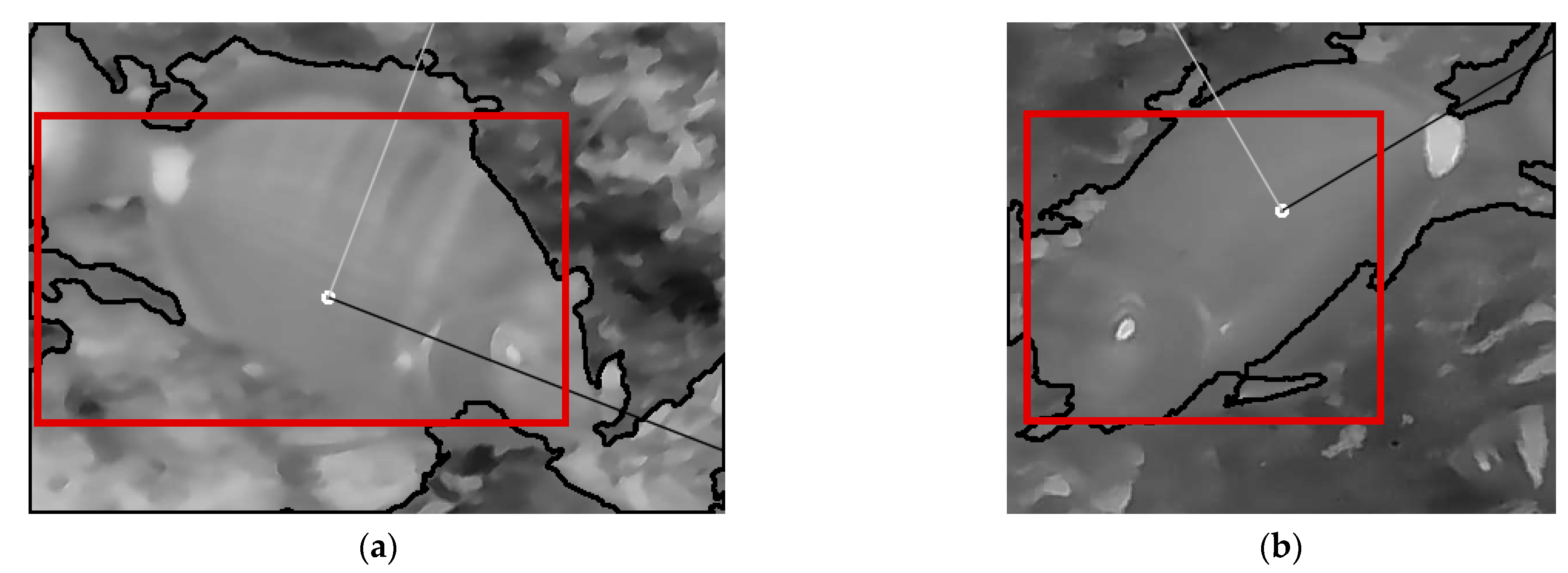
The image patch is inverted if the fish color is darker than its background. In order to detect the brightness of the fish, the average gray level of the internal part of the image is compared to that of the image border zone, separated by the red squares in Figure 5. The border zone is defined with a thickness of B=20 pixels. Having in mind that the image patches are actually bounding boxes of the detected fish, it is expected that most of the fish body is mainly displayed in the internal region while the background in the border zone. If the average gray color of the internal region (fish) is darker than that of the border zone (background) then, the image color is inverted as is the case in both images of Figure 5. Then, the image is segmented using Otsu’s threshold [37] and the contour surrounding the largest area is used as input to the OpenCV PCA method.
The output is an accurate estimation of the fish tilt axis but the direction is not detected accurately. Therefore, additional segmentation methods are deployed to determine the direction the fish is facing. Having in mind that the ERT model can detect shapes with a ±20o tilt, it is sufficient to classify fish captured from the side view in 4 different orientation categories: fish facing up-left (Q0), up-right (Q1), down-left (Q2) and down-right (Q3). We assume that fish cannot be captured in a 90o vertical tilt since it is not natural for a fish to swim in this direction. Using the anatomy of the fish it is expected that if most of the fish body is found in the left half of the image patch, the fish is facing left (Q0 or Q2), otherwise it is facing right (Q1 or Q3). This simple method is called hereafter Coarse Orientation Detection (COD). It is implemented by comparing the area of the fish body in the left and right areas of the image i.e., Q0+Q2 is compared to Q1+Q3. Symbols Q0, Q1, Q2 and Q3 are used to represent the number of pixels mapped to fish body in the corresponding quadrants. Extending this principle to the individual Q0, Q1, Q2, Q3 quadrants, a Fine Orientation Detection (FOD) takes place. If for example, the COD decides the fish is facing left then the fish is facing up-left if Q0>Q2 (i.e., the area of the fish in Q0 is higher than the area in Q2), otherwise it is facing down-left. The COD and FOD processes are demonstrated in Figure 6.
A fourth orientation detection method employed, is based on template matching. More specifically, a template of the fish eye is used to locate the position of the eye and consequently the orientation of the fish. Based on the resizing of the image patches described earlier and the fact that the fish have similar dimensions after resizing, a 30 × 30 pixel template of the eye is used. The OpenCV template matching procedure is repeated for resized eye templates of 28 × 28 and 32 × 32 pixels. The direction shown by the majority of the 3 template matching procedures is used as output of this orientation detection method. Figure 7 shows examples of successful and unsuccessful eye template matches. In some low contrast images the fish eye is not visible at all, while the eye template can easily match background objects or even other body parts such as the caudal fin of the diplodus annularis as shown in Figure 7d.
To improve the orientation classification accuracy of the 4 orientation detection methods described above, combinations of these methods can be examined as will be described in Section 3.

2.5. Fish Tracking

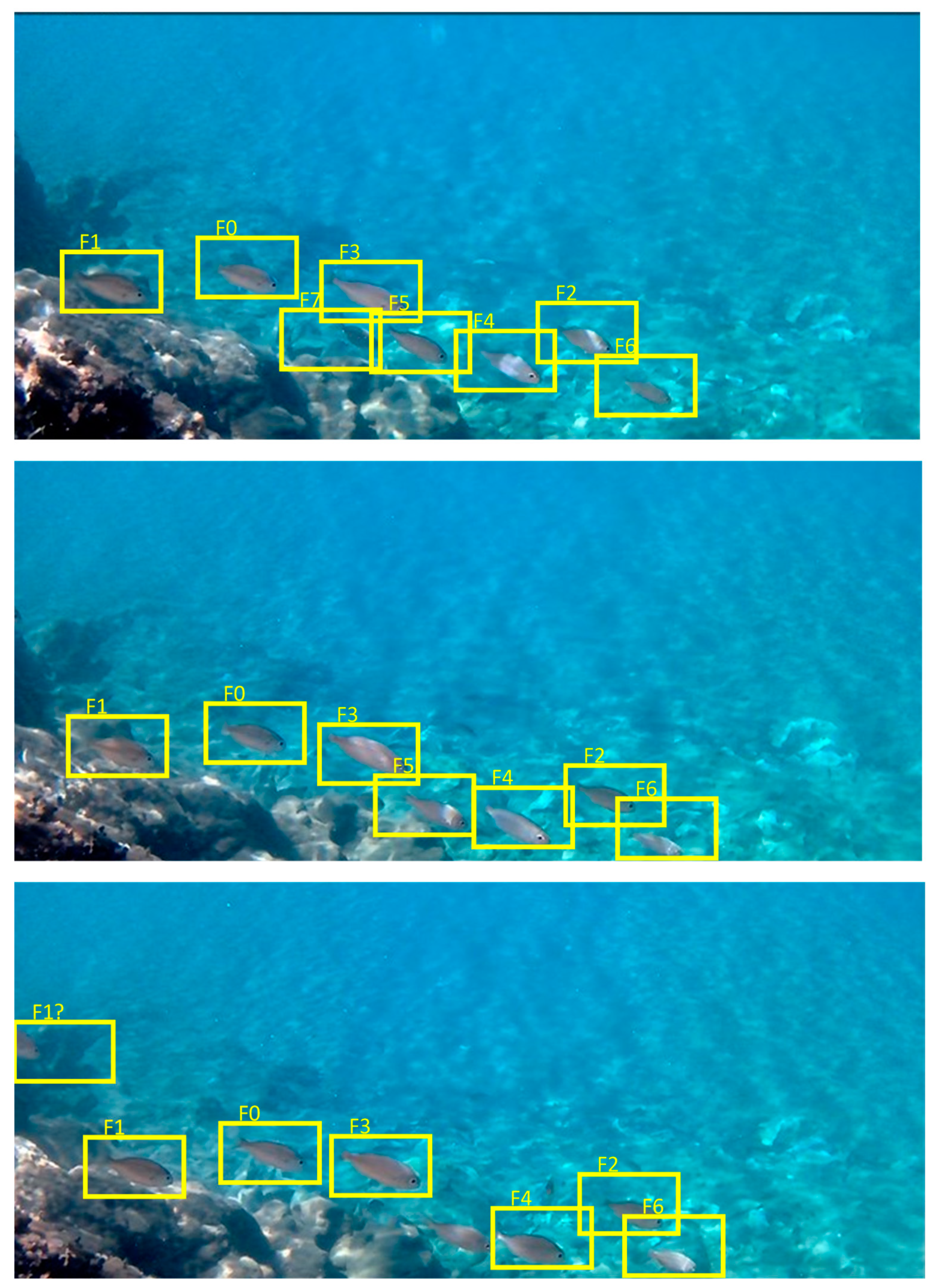
The fish tracking supported in the framework of this work registers the coordinates of the bounding boxes and orientations of the fish found in successive frames. The target is to determine the track of an individual fish and avoid confusion with tracks of other fish swimming in the neighborhood. To understand the concept of the adopted approach, the successive frames shown in Figure 8 can be considered. These frames have a time distance of 1 sec which is rather large and are captured from a camera that was not stable as required for the case of fish track monitoring. However, they contain a number of fish all facing in the same direction (down-left) making the explanation of the tracking algorithm easier. Let c i t be the coordinate pairs of the top left corner of the bounding box i in frame t. It is assumed that the bounding box j corresponding to the same fish in the next frame t+1 is the one that satisfies eq. (7), provided that the frames t and t+1 have a relatively short time distance e.g., less than 1 sec.
i = a r g m i n c j t + 1 c i t 2
If the time distance between these two frames is too long, the correspondence of bounding boxes with fish in the next frame may not be accurate since: a) the reference fish may have moved away and another one is now closer to the previous position of the reference fish and b) the reference fish may have changed direction, or orientation, etc. In the top frame of Figure 8, seven fish are detected (F0-F8). The new position of these fish is monitored in the next two frames of Figure 8.
The fish names in the middle and bottom frames of Figure 8 were assigned based on the Euclidean distances estimated in Table 1. In each frame, the coordinates of the top-left bounding box corners are listed for the fish detected in these frames. In the first frame, the bounding boxes are assigned to names F0 to F7. In the Frame 2, the top-left coordinates of each bounding box are used in eq. (7) to estimate its Euclidean distance from each one of the bounding boxes found in Frame 1. The shorter distance is used to assign fish names in the second frame as shown in the 4th column of Table 1. Each fish name is followed by its distance (in pixels) from the bounding box of the fish that it has been assigned to. Fish F7 was not recognized in Frame 2. Similarly, in Frame 3 the new bounding boxes are associated to the fish detected in Frame 2 using the shorter distances.
In Frame 3, fish F5 has not been recognized while a new fish appeared at the left side of the image and was associated to F1 since this fish is closer. For this reason, there are two bounding boxes associated with F1 and the system has to select which one actually corresponds to F1. The fish orientation is used to solve this issue. Since all the fish in the three frames are heading bottom-right the new fish that appeared from the left is not associated with the fish that appeared in Frames 1 and 2 and is assumed to be a new fish. The exploitation of the orientation features in fish tracking is triggered when a bounding box in the current frame is assigned to more than one fish detected in the next frame. Among the bounding boxes assigned to the same fish name, the one with the smaller distance and in the right direction is selected. Of course, if there is no ambiguity, the fish can change orientation in the current frame and its association with a fish in the previous frame is only determined by the Euclidean distance. On the other hand, the confirmed direction that the fish is following in the last frames, can also be exploited in the orientation classification and consequently in the morphological feature extraction stage to get more accurate results.
More features can also be taken into consideration for accurate track monitoring: a) the bounding boxes associated with fish from the previous frame should belong to fish of the same species, b) the size of the associated fish in successive frames should match, c) the position of the new bounding box should agree with the speed of the fish measured from previous frames. The study of how these features can be incorporated in our fish tracking procedure as well as its evaluation is part of our future work.

2.6. ERT Background

The face alignment method presented in [27] is based on a ML method called Ensemble of Regression Trees (ERT) and was originally used to align landmarks on human faces. We use this method to find the shape of a fish based on a set of 18 landmarks. When ERT is applied to a new image, the mean position of the landmarks stored in the trained model is gradually corrected in Tc cascade stages. In each cascade stage, Nr regression trees are visited. Each binary regression tree has 2Td-1 nodes and in each node the gray level of a pair of pixels from a sparse representation of the input frame is compared. The next node of the regression tree that has to be visited is selected according to the comparison results. A correction factor is found in the leaves of each regression tree and this factor is used to correct the current landmark positions.
Let S be the shape of the fish i.e., the set of 18 pairs of Cartesian coordinates, and S ^ t , the estimated shape at the cascade stage t (0≤t<Tc). In the next cascade stage t+1, the shape estimation S ^ t + 1 is updated from S ^ t with a correction factor rt:
S ^ ( t + 1 ) = S ^ ( t ) + r t
The correction factor rt is determined by the residuals between the current estimation and the trained shapes as well as the correction factors retrieved from the regression tree leaves. At the beginning of each cascade stage, the sparse image represented by Nr reference pixels is warped to match the shape of the fish within a process called Similarity Transform (ST). If q is a reference pixel and its neighboring landmark has index kq, their distance δxq is represented as:
δ x q = q x k q 2
The pixel q’ in the sparse input image that corresponds to q in the mean shape is estimated as:
q ' = x i , k q + 1 s i R i T δ x q
The parameters si and Ri are scale and rotation factors respectively, employed in the ST process to warp the fish shape. For more information, please see [27].

2.7. Shape Alignment for Fish Morphological Feature Extraction

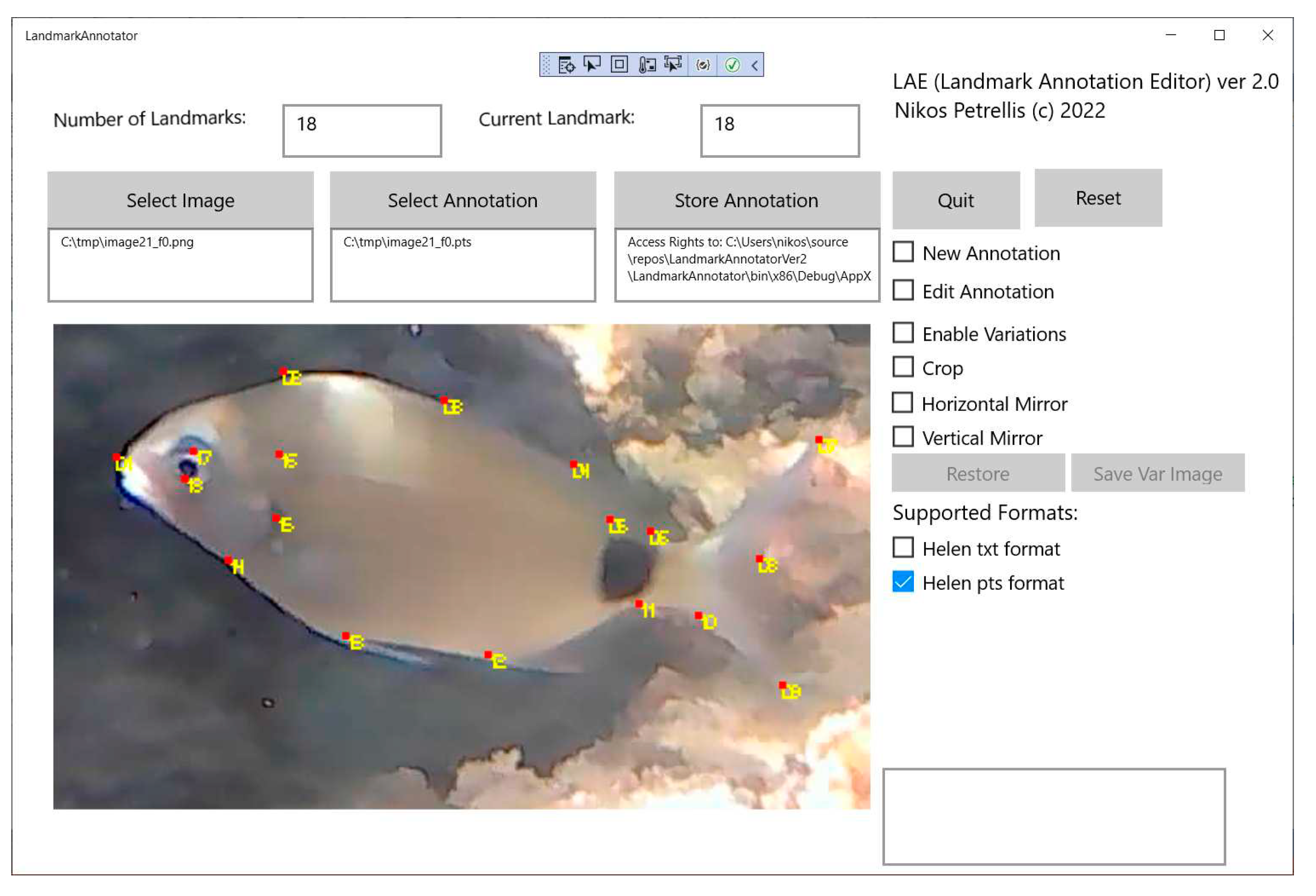
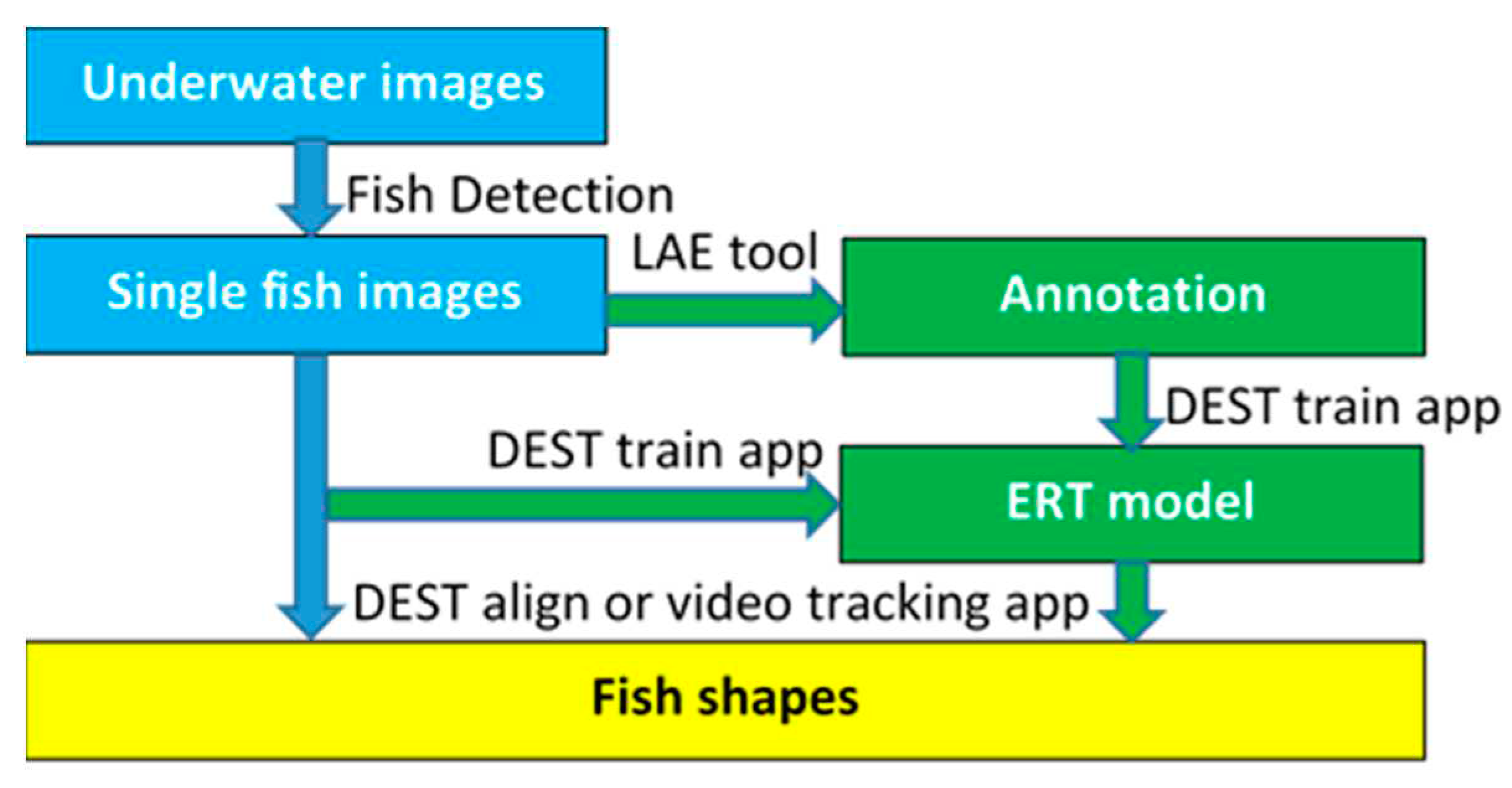
The ERT method described in the previous paragraph and its implementation in DEST [29] has been employed for fish shape alignment based on L=18 landmarks as shown in Figure 9. Landmark No. 1 marks the position of the fish mouth, landmarks 2-5, the upper part of the fish contour, landmarks 6-10, the perimeter of the caudal fin, landmarks 11-14, the lower part of the contour, landmarks 14-16, the position of the gill and finally landmarks 17-18, the position of the eye. These landmarks allow the estimation of relative fish dimensions and the location of regions of interest (ROIs) of the fish body, that are critical for the assessment of the fish health such as the eyes or the gills. The relative length of the fish can be determined as the distance (expressed in pixels) between landmarks No 1 and 8, while the relative height as the distance between landmarks No. 3 and 13. Absolute dimensions can be estimated if stereo vision is employed with a pair of cameras instead of a single one. More details on how this can be achieved, may be found in our previous work [31]. The fish shape malformations can also reveal information about the health of the fish, the specific species variation of the fish, its growing conditions, etc. The malformations can be indicated by the position of certain landmarks like the ones in the upper and lower part of the fish contour. A denser shape representation with more landmarks may be necessary to detect malformations or variations in the species. The developed framework can be trained to align fish shapes with any number of landmarks without any modification. The process that has to be followed is depicted in Figure 10.
The training on the target fish species requires a number of images, each one displaying a single fish. These images can be the patches generated by the fish detection phase in Figure 2, from underwater images. Each one of these single fish images should be accompanied by an annotation text file in order to perform the training procedure. A new Landmark Annotation Editor (LAE) has been developed that can be easily used to create or edit annotations of any number of landmarks. The format of the annotations created by the LAE editor is compatible with the one required by the suite of the DEST tools [29]. The main window of the LAE tool is shown in Figure 9. An image can be loaded in this editor and a new annotation can start or a stored one can be edited. Landmarks can be easily moved with a single mouse click. The annotation can be stored in one of the supported formats. The LAE tool offers a number of data augmentation functions (image crop and mirroring) that can be useful in the development of new training datasets. The dataset consisting of (fish image, annotation files) pairs are used for the training of an ERT model using the dest_train application of the DEST suite of tools.
The original DEST suite of applications [29] is written in C++ and has been ported in our previous work [30], in Ubuntu environment. The DEST application for video tracking has then been ported to a target Xilinx Vitis environment for hardware acceleration support in order to achieve a higher frame processing speed. Although the porting to the Ubuntu and Xilinx Vitis environment has been performed for human face alignment in the context of a driver drowsiness application, the tools already developed can be used without any modification for the alignment of other shapes like the fish shape described in this work. For more convenience, the DEST suite of applications has also been ported to Windows environment using Microsoft Visual Studio 2019.
The resulting ERT model that has been trained, can be used with other DEST applications like the one that aligns shapes in single photographs (dest_align) or the one that aligns shapes in video frames (dest_video_tracking). In the process of porting the DEST applications’ source code to both Ubuntu and Windows environments, a software restructuring took place that allowed an acceleration in the frame processing speed by more than 240 times: a 1920 × 1080 pixel frame processing latency was reduced from 116ms to 475us on an Intel 6-Core i5-9500 CPU running at 3.00GHz [29]. This significant acceleration in software was achieved by replacing time consuming calls to the Eigen math library [38] with optimized C code. The original DEST source code was calling Eigen template library functions for matrix/vector operations, Jacobi rotations, Singular Value Decomposition (SVD), etc. Using Eigen library and well defined C++ classes, ensures the integrity of the data values in any application and allows the operations to be described in a compact and portable way. However, excessive integrity checks and data type conversions were responsible for a high latency overhead. Moreover, the Eigen and C++ classes and data types used in DEST were not appropriate for hardware synthesis and implementation on reconfigurable hardware using state-of-the-art tools such as Xilinx Vitis.
If even higher frame processing speed is needed, the shape alignment latency can be further reduced by more than 50% if it is implemented on an embedded platform like a Xilinx ZCU102 development board with ZynqMP Ultrascale+ FPGA. Porting an ML method like ERT in hardware is not a typical hardware acceleration problem since a number of large arguments have to be passed to the kernel. Moreover, there are not many repetitive operations to be performed on this data. For this reason, the acceleration techniques have been focused in the reduction of the latency of bulk data transfers from the software (ARM processor) to the hardware kernel (FPGA). More details can be found in [30].

3. Experimental Results

A test set of P=100 fish photographs have been used to estimate the absolute error in the position of the landmarks compared to the annotation defined as ground truth in the LAE editor. The relative error εri between the estimated landmark k i ^ position and its corresponding position ki in the ground truth annotation is the Euclidean distance between these two positions, expressed in pixels:
ε r i = k i ^ k i 2
If k i = ( w i , h i ) and k i ^ = ( w i ^ , h i ^ ) and the image (width, height) is (w,h), the normalized relative error for landmark i, (εni) is:
ε n i = ( w i ^ w i ) 2 w 2 + ( h i ^ h i ) 2 h 2
The standard deviation (SD), σε in the distribution of the landmark estimation error εni across all L landmarks is:
σ ε = 1 L i = 1 L ( ε n i μ ε ) 2
where με is mean error of εni i.e.,
μ ε = 1 L i = 1 L ε n i
The standard deviation in the distribution of estimation error εnij of a specific landmark i in P images (0≤j<P) is:
σ i = 1 P j = 1 P ( ε n i j μ i ) 2
where μi is mean error of εnij i.e.,
μ i = 1 P j = 1 P ε n i j
Another standard deviation metric (σP) used is in the average relative error μεj (see eq. (14)) of all landmarks of an image in all the P test images:
σ P = 1 P j = 1 P ( μ ε j μ P ) 2
where μP is the mean of μεj:
μ P = 1 P j = 1 P μ ε j
Table 2, shows the average, minimum and maximum, absolute and relative errors that have appeared in all landmarks and all the P test images.
The standard deviation σε limits as well as the σP deviation of the average error in the P test images are listed in Table 3.
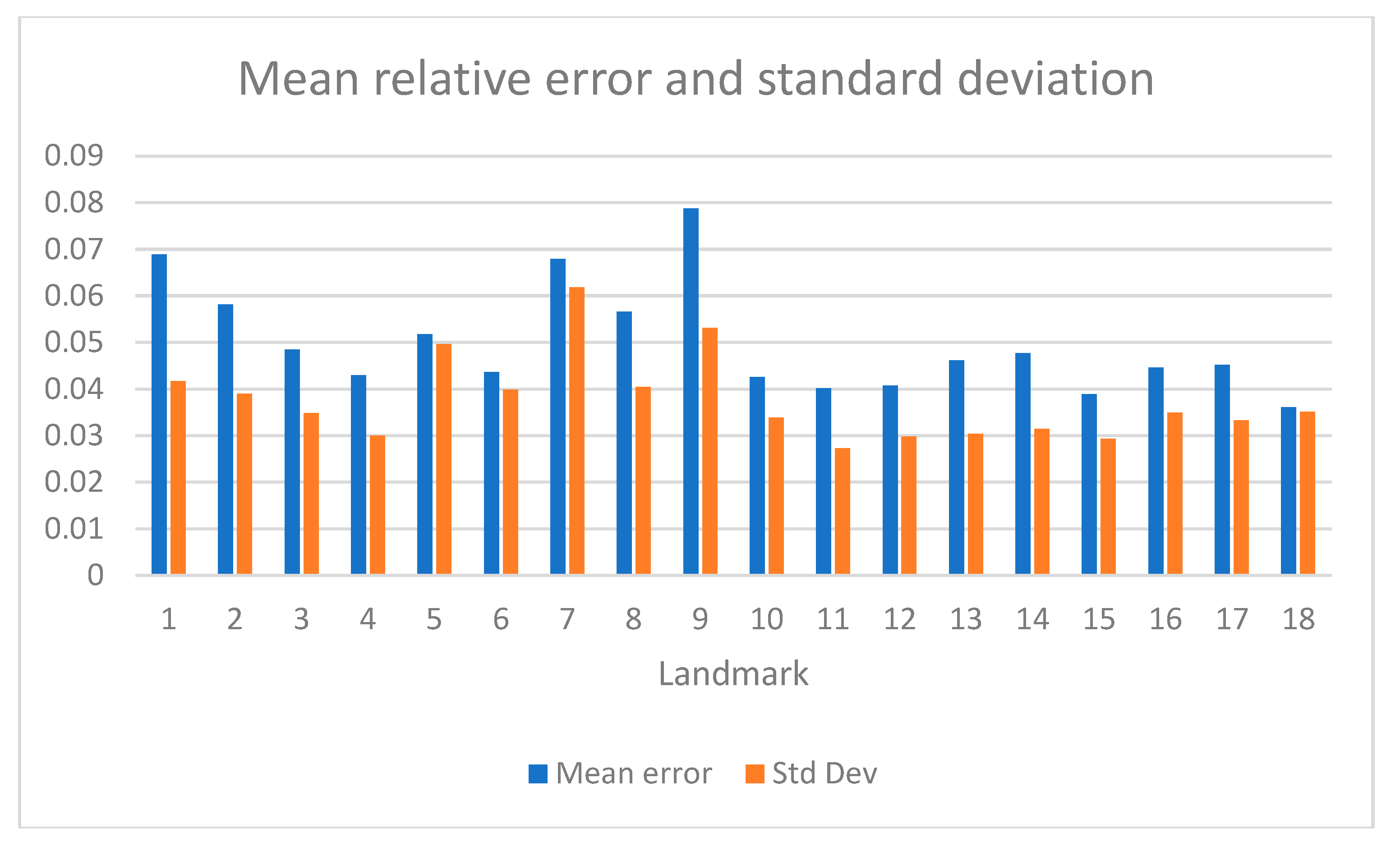
The mean error μi of each landmark i, along with its standard deviation σi is plotted in Figure 11. This plot is of particular interest because it highlights the landmarks that show the highest error.
The error in the relative height and length estimation of the fish in the test set is listed in Table 4 along with their standard deviations.
Concerning the fish orientation methods described in Subsection 2.4, Table 5 lists the success rates achieved with each method. The PCA method is capable of recognizing the fish tilt with a very good accuracy (less than ±10o in more than 95% of the cases). However, the direction that the fish is facing, is recognized with much lower accuracy as shown in Table 5. COD performs a draft classification in left or right direction, while FOD performs a more detailed orientation classification in quadrants Q0-Q3 with the success rate listed in Table 5. Eye template matching (TM) is also used to classify the direction in one of the Q0-Q3 quadrants. Then, a number of combinations of these orientation classification methods are tested.
In PCA+COD, the tilt found by PCA is used while COD is used to detect the direction. In PCA+COD (2), COD direction is taken into consideration only if the confidence is above a threshold. In PCA+TM the coarse left-right direction indicated by TM is taken into consideration to decide the direction on the tilt estimated by PCA. If, for example, the tilt is from bottom-left to top-right, then Q1 is selected if TM finds the fish eye in the right quadrants (Q1, Q3). If the fish eye is found in the left quadrants (Q0, Q2), then Q2 is selected. In PCA+TM (2) method the TM direction is considered only if the template matching found the fish eye in one of the quadrants that are compatible with the fish tilt indicated by PCA. For example, if the fish is facing up-right, its caudal fin is in Q2 and its head is in Q1. If the TM method finds the fish eye in Q1 or Q2 then, the direction indicated by TM will be assumed correct. Specifically, with fish eye found by TM in Q1 it will correctly be recognized that the fish is facing up-right while if the fish eye is found in Q2 it will be assumed by mistake that the fish is facing down-left. If the TM finds the fish eye in Q0 or Q3, the direction indicated by TM will not be taken into consideration and only the direction indicated by PCA will be used.
In Table 6, a comparison can be found between our fish length estimation method and the references that present fish size estimation results.

4. Discussion

From the experimental results presented in the previous section, it was shown that the average relative error in the alignment of a single landmark is 4.8% (corresponding to an absolute error of 17.54 pixels) with the following SDs: σε=0.03, σΡ=0.0215. When estimating specific fish body dimensions, the relative error is 5.4% in the length and 5.5% in the height (with the corresponding SD being 0.049 and 0.062, respectively). Taking into consideration that the length of the fish recognized in the photographs of the dataset ranges from 10cm to 20cm, the average absolute error is in the order of 0.5cm-1cm.
From Figure 11, more details can be seen about the accuracy in the alignment of individual landmarks. For example, landmarks 7 (top of the caudal fin) and 9 (bottom of the caudal fin) are located with a mean error equal to 6.8% and 7.8%, respectively. These are the highest relative errors measured per landmark. They appear at the landmarks that mark the edge of the caudal fin because in most photographs of the dataset used for training and testing, the caudal fin perimeter is often indistinguishable from the background. Landmarks 1 (mouth) and 8 (middle of the caudal fin), that are used for the estimation of fish length are located with a mean error of 6.8% and 5.6%, respectively. When they are combined to estimate the fish length, the average relative error is 5.4%.
Landmarks 3 and 13 are used to estimate fish height. Their average relative error is 4.8% and 4.6%, lower than the error shown by landmarks 1 and 8 that have been used for length estimation. However, when they are combined to estimate fish height, the average relative error measured is a little higher (5.5%) than that of the fish length (5.4%). Other landmarks of interest are No. 17 and 18 that are used to locate the fish eye ROI. These landmarks are located with an average relative error of 4.5% and 3.6%. Taking into consideration the fish size range mentioned above, this relative error in the fish eye localization is translated to about 0.4cm-0.8cm. Although it is not always safe to assume that the fish eye is within landmarks No. 17 and 18, additional pattern recognition methods can be applied to detect accurately the shape of the eye near the area indicated from these landmarks. Similarly, the gills’ area is another ROI located by landmarks No. 14, 15 and 16. The mean relative errors in the estimation of the position of these landmarks range between 3.8% and 4.7%.
Concerning the fish orientation classification, Table 5 shows that the best results are achieved with the combination of PCA with TM when the false eye template matching estimations are ignored. PCA is capable of detecting with a high accuracy the tilt of the fish. However, it could detect the direction of the fish in only 44.8% of the times, using the low contrast images of the developed dataset. The COD achieved a higher success rate (67.2%) but can detect only a draft left or right direction. The FOD method could be used to classify the direction of the fish in four quadrants but its classification accuracy is only 43.1%. On the other hand, fish eye template matching has a relatively higher success rate of 63.8%. This could have been even higher, if the resolution and the quality of the dataset images was better because in many fish image patches the eye is not visible at all. In these cases, the eye is confused either with background objects or with other parts of the fish like a strip in the caudal fin of some species like Diplodus annularis. Certain combinations of these orientation detection methods were also tested as shown in Table 5. Combining PCA with the left or right classification of COD achieved a success rate of 65.5%. The highest accuracy was achieved when the PCA was combined with TM and can reach 79.3%. A much higher orientation accuracy is expected to be achieved if the track of the fish is also taken into consideration at explained in subsection 2.5.
Comparing the fish size estimation methods listed in Table 6, it is obvious that the proposed fish length or height estimation achieves one of the highest accuracies. In [17], a slightly lower error (5%) is achieved while in [23] the error is lower only in some specific fish sizes. However, in most of the cases presented in the literature, fish size is estimated in a controlled environment (e.g., on a conveyor belt) or with high resolution underwater images. Estimating fish size in low contrast and low quality images like the ones of the dataset used, is a much more challenging task.
Summarizing, the developed framework offers a number of useful services for fish monitoring such as morphological feature estimation, fish orientation classification and fish tracking. These services can be useful both for monitoring fish in free waters and aquacultures. The fish detection, orientation classification and shape alignment methods for morphological feature estimation were described in detail. The principles of fish tracking in the developed framework were also discussed.
One of the limitations of the current work is the latency of the fish detection. Specific directions were given to pipeline the fish detection in specific frames with other tasks that can run in parallel threads. These tasks can be the bounding box interpolation in intermediate frames between actual fish detections, the execution of the orientation methods and the shape alignment. Shape alignment is already available with hardware acceleration on embedded platforms. Similarly, the neural network for the inference that performs fish detection can also be implemented in hardware on the same target platform. Developing such an architecture is part of our on-going work in order to achieve a high frame processing speed and real time operation.
Finally, more sophisticated techniques can also be incorporated in the presented fish tracking approach. For example, feedback from the shape tracking stage can be used to identify with higher confidence the fish in successive frames without confusing their positions. The fish orientation can also indicate when the fish is changing direction in its track.

5. Conclusions

Fish detection, orientation classification, size estimation, locating regions of interest and fish tracking is supported in the developed framework, presented in this paper. It can be exploited for fish monitoring in aquacultures and open seas. It is based on deep learning for fish detection, OpenCV services for orientation classification and the adaptation of a shape alignment machine learning method called Ensemble of Regression trees. The fish detection is performed with an accuracy higher than 95% since in all cases, almost all of the fish that are expected to be monitored, were detected. The orientation of the fish is classified in four major directions with 80% success rate. The relative fish size estimation was also performed with 5.5% accuracy.
Future work will focus on employing hardware acceleration for the fish detection inference, in order to achieve high frame processing speed and real time operation. Moreover, the employed fish tracking method will be improved with enhanced techniques that will detect the speed and the changes in the direction of the fish.

Supplementary Materials

A description of how DEST was ported to Ubuntu environment and MS Visual Studio 2019 as well as the use of LAE editor can be found in the videos of the playlist https://www.youtube.com/playlist?list=PLXUuQj2gQ4s9TXI12kP9WMaxthWrjAweF. The description of how hardware acceleration has been applied to DEST video tracking application for face shape alignment can be found in https://youtu.be/OlCBCwroAkw.

Author Contributions

Conceptualization, N.P. and G.K.; methodology, N.P.; software, N.P.; validation, N.P. and G.K; resources, C.A. and N.V.; data curation, N.P.; writing—original draft preparation, N.P.; writing—review and editing, all; supervision, N.V.; project administration, N.P. and N.V. All authors have read and agreed to the published version of the manuscript.

Funding

This research received no external funding.

Data Availability Statement

The dataset used will soon be publically available.

Acknowledgments

The authors wish to thank the student Spilios Kostopoulos for conducting part of the experiments

Conflicts of Interest

The authors declare no conflict of interest.

References

  1. Vo, T.T.E.; Ko, H.; Huh, J.-H.; Kim, Y. Overview of Smart Aquaculture System: Focusing on Applications of Machine Learning and Computer Vision. Electronics 2021, 10, 2882. [Google Scholar] [CrossRef]
  2. Zion, B. The use of computer vision technologies in aquaculture—A review. Computers and Electronics in Agriculture 2012, 88, 125–13. [Google Scholar] [CrossRef]
  3. Mathiassen, J.R.; Misimi, E.; Bondø, M.; Veliyulin, E.; Østvik, S.O. Trends in application of imaging technologies to inspection of fish and fish products. Trends in Food Science & Technology 2011, 257–275. [Google Scholar] [CrossRef]
  4. Franceschelli, L.; Berardinelli, A.; Dabbou, S.; Ragni, L.; Tartagni, M. Sensing Technology for Fish Freshness and Safety: A Review. Sensors 2021, 21, 1373. [Google Scholar] [CrossRef]
  5. Freitas, J.; Vaz-Pires, P.; Câmara, J.S. From aquaculture production to consumption: Freshness, safety, traceability and authentication, the four pillars of quality. Aquaculture 2020, 518, 734857. [Google Scholar] [CrossRef]
  6. Choi, J.W.; Jang, M.K.; Hong, C.W.; Lee, J.W.; Choi, J.H.; Kim, K.B.; Xu, X.; Ahn, D.H.; Lee, M.K.; Nam, T.J. Novel application of an optical inspection system to determine the freshness of Scomber japonicus (mackerel) stored at a low temperature. Food Sci Biotechnol 2020, 29, 103–107. [Google Scholar] [CrossRef]
  7. Dowlati, M.; Mohtasebi, S.S.; Omid, M.; Razavi, S.H.; Jamzad, M.; De La Guardia, M. Freshness assessment of gilthead sea bream (Sparus aurata) by machine vision based on gill and eye color changes. J. Food Eng. 2013, 119, 277–287. [Google Scholar] [CrossRef]
  8. Li, X.; Shang, M.; Qin, H.; Chen, L. Fast accurate fish detection and recognition of underwater images with Fast R-CNN. Oceans 2015, 1–5. [Google Scholar] [CrossRef]
  9. Jalal, A.; Salman, A.; Mian, A.; Shortis, M.; Shafait, F. Fish detection and species classification in underwater environments using deep learning with temporal information. Ecological Informatics 2020, 57, 101088. [Google Scholar] [CrossRef]
  10. Sung. M. Vision based real-time fish detection using convolutional neural network. Oceans 2017, 1–6. [CrossRef]
  11. Xie, Y. Improved Gaussian Mixture Model in Video Motion Detection. Journal of Multimedia 2013, 8, 527–533. [Google Scholar] [CrossRef]
  12. Lekunberri, X.; Ruiz, J.; Quincoces, I.; Dornaika, F.; Arganda-Carreras, I.; Fernandes, A.A. Identification and measurement of tropical tuna species in purse seiner catches using computer vision and deep learning. Ecological Informatics 2022, 67, 101495. [Google Scholar] [CrossRef]
  13. He, K.; Gkioxari, G.; Dollár, P.; Girshick, R. Mask R-CNN. Available online https://arxiv.org/abs/1703.06870. (accessed on 25 May 2023).
  14. He, K.; Zhang, X.; Ren, S.; Sun, J. Deep Residual Learning for Image Recognition. In Proceedings of the 2016 IEEE Conference on Computer Vision and Pattern Recognition (CVPR), Las Vegas, NV, USA, 27–30 June 2016; pp. 770–778. [Google Scholar] [CrossRef]
  15. Qin, H.; Li, X.; Liang, J.; Peng, Y.; Zhang, C. Deepfish: accurate underwater live fish recognition with a deep architecture. Neurocomputing 2016, 187, 49–58. [Google Scholar] [CrossRef]
  16. Sun, X.; Shi, J.; Dong, J.; Wang, X. Fish recognition from low-resolution underwater images. Proceedings of 9th IEEE International Congress on Image and Signal Processing, BioMedical Engineering and Informatics (CISP-BMEI), 471–476, Datong, China, 15–17 October 2016. [Google Scholar] [CrossRef]
  17. Ubina, N.A.; Cheng, S.C.; Chang, C.C.; Cai, S.Y.; Lan, H.Y.; Lu, H.Y. Intelligent underwater Stereo Camera Design for Fish Metric Estimation Using Reliable Object Matching. IEEE Access 2022, 10, 74605–74619. [Google Scholar] [CrossRef]
  18. Fisher, M.H.; French, J.; Gorpincenko, A.; Mackiewicz, M.; Holah, H.; Clayton, L.; Selkow, R. Motion Stereo at Sea: Dense 3D Reconstruction from Image Sequences Monitoring Conveyor Systems on Board Fishing Vessels. IET Image Processing 2022. [Google Scholar] [CrossRef]
  19. Karnani, K.; Pepper, J.; Bakis, Y.; Wang, X.; Bart, H.; Breen, D.; Greenberg, J. Computational Metadata Generation Methods for Biological Specimen Image Collections. , PREPRINT (Version 1) available at Research Square. 27 April. [CrossRef]
  20. Kandimalla, V.; Richard, M.; Smith, F.; Quirion, J.; Torgo, L.; Whidden, C. Automated Detection, Classification and Counting of Fish in Fish Passages With Deep Learning. Front. Mar. Sci. 2022, 8, 823173–10. [Google Scholar] [CrossRef]
  21. Alori, J.; Descoins, A.; Ríos, B.; Castro, A. Norfair Library. tryolabs/norfair: v0.3.1. Available online: https://doi.org/10.5281/zenodo.5146254 (accessed on 25 May 2023).
  22. Bochkovskiy, A.; Wang, C. Y.; Liao, H. Y. M. Yolov4: Optimal speed and accuracy of object detection. arXiv 2020, arXiv:2004.10934. [Google Scholar]
  23. Martignac, F.; Daroux, A.; Bagliniere, J.L.; Ombredane, D.; Guillard, J. The use of acoustic cameras in shallow waters: new hydroacoustic tools for monitoring migratory fish population. A review of DIDSON technology. Fish and Fisheries 2015, 16, 486–510. [Google Scholar] [CrossRef]
  24. Terayama, K.; Shin, K.; Mizuno, K.; Tsuda, K. Integration of sonar and optical camera images using deep neural network for fish monitoring. Aquacultural Engineering 2019, 86, 102000. [Google Scholar] [CrossRef]
  25. Fish detection. Available online: https://github.com/kwea123/fish_detection (accessed on 1 March 2023).
  26. OpenCV. Available online: https://opencv.org/ (accessed on 25 May 2023).
  27. Kazemi, V.; Sullivan, J. One millisecond face alignment with an ensemble of regression trees. In Proceedings of the IEEE Conference on Computer Vision and Pattern Recognition, Columbus, OH, USA, 23–28 June 2014; pp. 867–1874. [Google Scholar] [CrossRef]
  28. Dlib C++ library. Available online: http://dlib.net/ (accessed on 25 May 2023).
  29. Deformable Shape Tracking (DEST). Available online: https://github.com/cheind/dest (accessed on 25 May 2023).
  30. Petrellis, N.; Christakos, P.; Zogas, S.; Mousouliotis, P.; Keramidas, G.; Voros, N.; Antonopoulos, C. Challenges Towards Hardware Acceleration of the Deformable Shape Tracking Application. In Proceedings of the 2021 IFIP/IEEE 29th International Conference on Very Large Scale Integration (VLSI-SoC), Singapore, Singapore, 4–7 October 2021. [Google Scholar] [CrossRef]
  31. Petrellis, N. Measurement of Fish Morphological Features through Image Processing and Deep Learning Techniques. Appl. Sci. 2021, 11, 4416. [Google Scholar] [CrossRef]
  32. Chyrka, I.; Kharchenko, V. 1D direction estimation with a YOLO network. In Proceedings of the 2019 European Microwave Conference in Central Europe (EuMCE), Prague, Czech Republic, 13–15 May 2019; pp. 358–361. [Google Scholar]
  33. Hara, K.; Vemulapalli, R.; Chellappa, R. Designing Deep Convolutional Neural Networks for Continuous Object Orientation Estimation. arXiv:1702.01499. [CrossRef]
  34. Song, F.; Guo, Z.; Mei, D. Feature selection using principal component analysis. In Proceedings of the 2010 International Conference on System Science, Engineering Design and Manufacturing Informatization, Yichang, China, 18 November 2010; pp. 27–30. [Google Scholar] [CrossRef]
  35. De Silva A. Object Orientation Detection and Correction using Computer Vision. Culminating Projects in Computer Science and Information Technology. 33. St. Cloud State University, 2020. https://repository.stcloudstate.edu/csit_etds/33.
  36. Lendave, V. Detecting Orientation of Objects in Image using PCA and OpenCV. Available online: https://analyticsindiamag.com/detecting-orientation-of-objects-in-image-using-pca-and-opencv/ (accessed on 15 May 2023).
  37. Otsu, N. A threshold selection method from gray-level histograms. IEEE Trans. Sys. Man. Cyber 1979, 9, 62–66. [Google Scholar] [CrossRef]
  38. Eigen 3.3.9. Available online: https://eigen.tuxfamily.org/ (accessed on May 15, 2023).
Figure 1. Fish patches extracted from a 4608 × 3456 resolution photograph (a) and from a 3840 × 2160 resolution video frame (b).
Preprints 76335 g001
Figure 2. The architecture of the developed system for fish monitoring and morphological feature extraction.
Preprints 76335 g002
Figure 3. Fish movement in video frames with time distance of 2 seconds.
Preprints 76335 g003
Figure 4. Fish Detection Interpolation (FPI).
Preprints 76335 g004
Figure 5. The Segmentation of the image using OpenCV Otsu threshold and applying PCA with m=2 to get the angles of the eigenvectors with the higher magnitude (black and white line). In both images the tilt denoted by the black line is recognized successfully but the direction in (a) is correct while in (b) is incorrect.
Preprints 76335 g005
Figure 6. COD and FOD methods. (a) Q0+Q2>Q1+Q3 (COD: fish facing left), Q0>Q2 (FOD: fish facing Up-Left. (b) Q1+Q3>Q0+Q2 (COD: fish facing right), Q3>Q1 (FOD: fish facing Down-Right).
Preprints 76335 g006
Figure 7. Fish eye template (a), successful matching in (b) and (c), caudal fin confused with fish eye in (d) and background object confused with fish eye in (e).
Preprints 76335 g007
Figure 8. Monitoring fish in 3 successive frames.
Preprints 76335 g008
Figure 9. Fish shape alignment based on 18 landmarks and the developed LAE landmark annotator.
Preprints 76335 g009
Figure 10. Fish shape alignment and training procedure.
Preprints 76335 g010
Figure 11. The mean relative error and standard deviation for each one of the 18 landmarks.
Preprints 76335 g011
Table 1. Association of the coordinates of the bounding boxes detected in Frames 2 and 3 with the fish detected in Frame 1.
Fish Frame1 Frame1 Y Frame1X Fish Frame2 Frame2 Y Frame2 X Fish Frame3 Frame3
Y
Frame3
X
F0 186 164 F0 (12) 197 165 F3(12) 206 250
F1 190 63 F3(52) 207 238 F0(11) 197 176
F2 231 409 F1(14) 203 69 F1(8) 211 71
F3 190 242 F2(14) 242 418 F2(23) 243 441
F4 246 353 F4(13) 259 355 F6(10) 276 474
F5 230 285 F6(12) 280 464 F1(104) 117 10
F6 269 459 F5(21) 249 295 F4(10) 265 364
F7 231 254
Table 2. Global absolute and relative errors.
Type of Error Error
Min Absolute Error 0.36 pixels
Max Absolute Error 78.33 pixels
Average Absolute Error 17.54 pixels
Min Relative Error 0.1%
Max Relative Error 33.6%
Average Relative Error 4.8%
Table 3. Relative error standard deviation σε limits and σP.
Parameter Value
Min σε deviation 0.0068
Max σε deviation 0.081
Average σε deviation 0.03
σP deviation 0.0215
Table 4. Error and standard deviation in measuring relative fish length and height.
Parameter Value
Fish length error 5.4%
Length error deviation 0.049
Fish height error 5.5%
Width error deviation 0.062
Table 5. Success rate in fish direction recognition with PCA, left or right direction classification with COD, classification in Q0-Q3 quadrants with FOD, template matching (TM) and their combinations.
PCA COD FOD TM PCA+COD PCA+COD (2) PCA+TM
Success Rate: 44.8% 67.2% 43.1% 63.8% 65.5% 65.5% 77.6%
Table 6. Fish size estimation comparison.
Reference Description Error
[12] Tuna fish size estimation SD: 0.328-0.396
[17] Fish length estimation Error 5%
[18] Fish size estimation Error 8%
[23] Fish length estimation Error 2%-8% depending on the fish size
This work Fish length estimation Error 5.4%
SD: 0.049
Disclaimer/Publisher’s Note: The statements, opinions and data contained in all publications are solely those of the individual author(s) and contributor(s) and not of MDPI and/or the editor(s). MDPI and/or the editor(s) disclaim responsibility for any injury to people or property resulting from any ideas, methods, instructions or products referred to in the content.
Copyright: This open access article is published under a Creative Commons CC BY 4.0 license, which permit the free download, distribution, and reuse, provided that the author and preprint are cited in any reuse.
Prerpints.org logo

Preprints.org is a free preprint server supported by MDPI in Basel, Switzerland.

Subscribe

© 2024 MDPI (Basel, Switzerland) unless otherwise stated