1. Introduction
A limestone quarries mine is used for the extraction of limestone, which is a useful non-metallic mineral in several mineral industries. It is a raw ingredient used in the cement industry. Drilling and Blasting is the significant excavation method of limestone quarry mine compared to the mechanical excavation methods. Blasting operations take place to breakdown the rock material into the desired size and we call that fragmentation, which is defined as the extent to which a rock mass or rock sample is broken into small pieces either primarily by mechanical tools, blasting, caving, and hydraulic fracturing or secondary by the breakage happened in loading and transportation of the material to the mill [
1]. Oversize of fragmented material and small-sized blasts lead to indirect cost escalation, unmanageable digging, and transportation of blasted muck pile, improper throw of fragmented rock material, ground vibration, fly rock at the time of blasting, and generation of overbreak [
2].
Most of the time it is stated that rock blasting operation is a way of producing fragmentation in mining and construction areas. The fragmented material produced by blasting has a great influence on mining and construction in different aspects. [
3] Cited from [
4] that in mining and processing plants, rock fragmentation distribution has high influences on loading, hauling, crushing rate, crushing, grinding capabilities, and ore recovery in beneficiation processes. According to [
5], the best fragmentation is a “blasting approach that offers the degree of fragmentation required to accomplish the lowest unit cost of the combined activities of drilling, loading, conveying, and crushing." Optimizing rock fragmentation results in increased excavator productivity, lower maintenance and repair costs for machinery used in loading and crushing operations, increased crusher productivity, and an impact on the complete process from start to finish, known as mine to the mill [
6], [
7]. The fragmented rock should be easily handled by the loading equipment and should fit with the available crusher/plant [
8].
Prediction of fragmentation has a great role in the optimization of rock fragmentations by finding the accuracy of the result with the presence of exact values. It has been observed by different researchers those different empirical methods like the kuz-Ram model, Kuznetsov’s equation, Rosin-Rammler’s equation, Cunningham’s uniformity index, and Modified Kuz-Ram model have been used to predict and improve the fragmentations resulting from blasting [
9]–[
12]. The kuz-Ram model is one of the approaches used for the prediction of rock fragmentation due to blasting. In the Kuz-Ram model, the input data consists of the relevant blast design parameters. Three key equations are the backbone of this equation, and these equations are Kuznetsova's equation, the Rosin-Rammler equation, and the uniformity index. The formula was created by Kuznetsov and further developed by Cunningham [
13]. [
10] Stated the Kuz-Ram model, not as a quantitative prediction model, but as a tool to examine how different parameters could influence blast fragmentation. A uniformity index is introduced later due to the deficiency of the model to describe the distribution of the fine, below the mean size. It is hypothesized that the finer fractions are produced by the pulverizing or crushing action of the explosive in a blast hole. The crushing zone radius around each blast hole is determined based on the peak blast-hole pressure and the strength of the rock [
14].
In this research, Artificial Neural Network (ANN) in comparison with machine learning models i.e., Random Forest regression (Bagging), Support vector regression, and XG Boost regression (Boosting) are used for the prediction of fragmentation. An artificial neural network (ANN) is a computational model mostly used for nonlinear fittings, which can simulate structures and functions of the biological neural network. ANN works by connecting various processing units and it can mimic how a human brain works. It is composed of many neurons of highly interconnected structure which can capable of performing massively parallel computations for data processing and knowledge representation to perform the desired functions [
15]–[
18].
Rock breakage mechanism and factors affecting rock fragmentation: Rock breaking due to blasting is a mechanism for breaking rock by producing shock waves and stress waves through detonations of an explosive placed in a drilled hole. The explosive placed inside the rock is detonated to impact the surrounding rocks and occurs in three phases. The first phase is a shock wave produced from the detonated explosive that applies strong impact and crushes the rock near the explosive charge (surrounding the holes). The second phase deals with stress wave damping, which is caused by shock waves moving outward from the blast hole in the rock [
19], [
20]. [
21]Stated about shock wave interaction in the presence of a short delay for the improvement of fragmentation, when the delays were in the range of contacts compared with no shock wave interactions, the results showed no clear differences or significant improvements in the fragmentation.
The stress waves break the rock by propagating in it in radial directions and forming a radial crack and spalling when they are reflected from a free face. [
22] claims that shock wave interactions are always extremely limited, affecting just a small portion of the Aside from proper blast geometry and effective stemming, the different properties of an explosive play a role in achieving optimal fragmentation [
25], [
26]. We can choose the types of explosives according to their properties by correlating them with the rock conditions that can fit. Some of the properties of the explosive which may affect the fragmentation are energy content, gas volume, detonation velocity, density, etc. It is necessary to consider its environment to get a satisfactory picture of an explosive's rock blasting performance because the useful energy released by the explosive depends on a lot of factors like the properties of the explosive, overall volume and that stress waves in the field never have similar shapes. The third phase is the extension of the cracks formed in the second phase to break the rock and move the broken rock in a direction toward the free face. This is carried out by the gases produced behind the detonation front, which are called gas energy. The pressure of gases helps in the final breakdown of the rock by extending cracks and increasing the volume of rocks. The broken rock always moves in a direction toward the free face [
23].
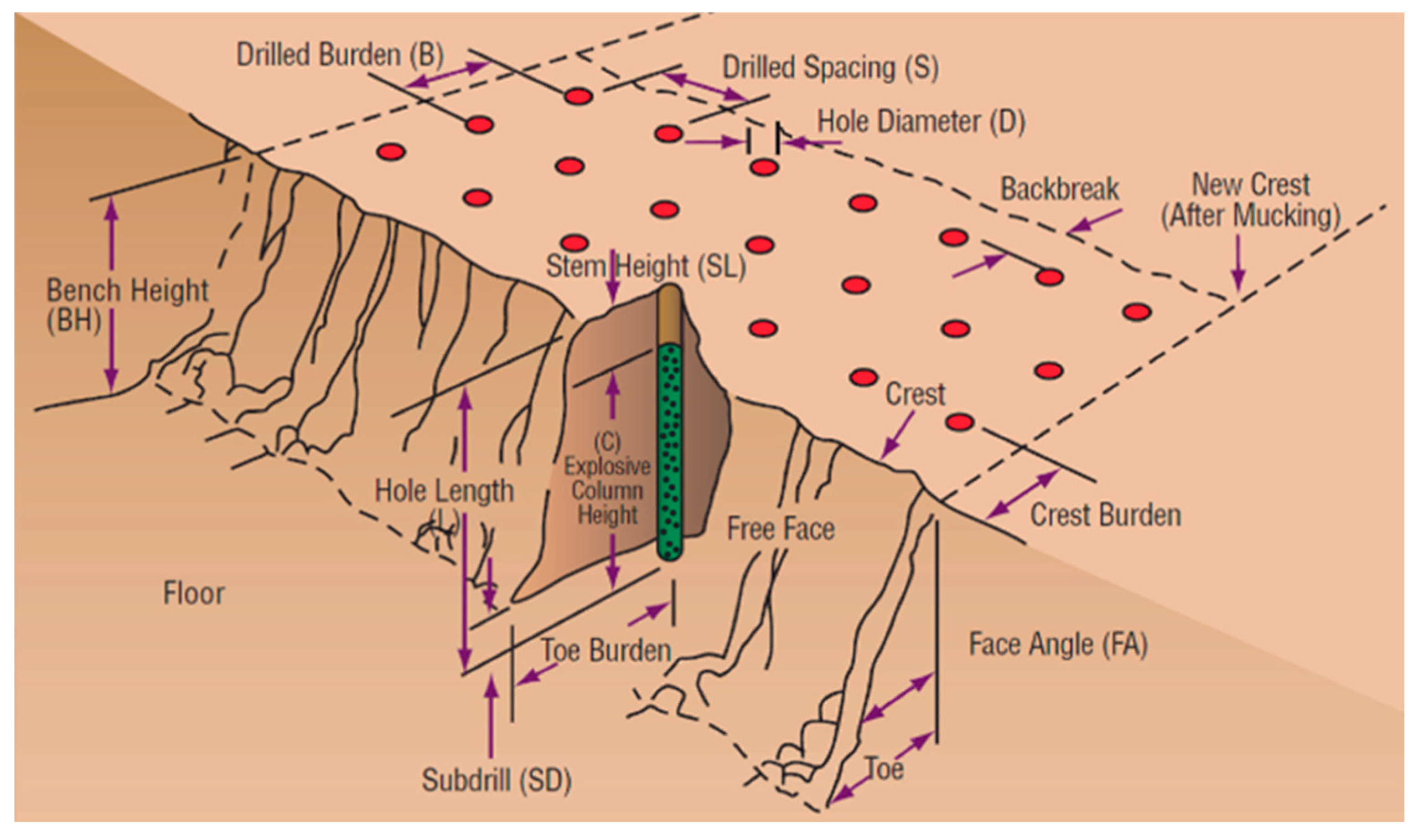
Factors affecting rock fragmentation: Different researchers explained that fragmentation is the breakage of rock material either using mechanical excavation or drilling and blasting operations. This outcome of blasting, which is called fragmentation, is influenced by several factors. Some are well-known, while others are more difficult to grasp. The conditions of the rock are of great importance, which means that the influence of changes in other factors can vary considerably from one place to another. A change in a parameter in one type of rock, for instance, can make an important difference in the result, whereas the same change in other places may not be noticed at all. They classified the factors into two big categories: controllable and uncontrollable parameters. The main controllable parameters are blast design parameters, which can differ from one blasting operation to the next and are used to modify and adjust the output of the operations to give us preferable results. They stated that the controllable parameters are classified into various groups. These groups are geometric parameters, which include burden, spacing between boreholes, bench height, drill hole diameter, hole length, charge depth, stemming height, sub-drilling, the drilling pattern, hole inclination (vertical or inclined), blasting direction, explosive parameters (types of explosives, energy, strength, priming systems, etc.), and time (delay timing and initiation sequence) [
24]. confinement of the explosive, i.e., properties of the rock, hole diameter, and degree of coupling. The more predictable fragmentation resulted in explosive VOD being high. This is achieved due to an increase in explosive energy, which corresponds to an increase in fragmentation [
27]. [
19] observed that the results of blasting operations are determined by a different parameter. Jimeno stated that poor fragmentation, insufficient swelling of the muck pile, uncontrolled fly rock, high vibration levels, and low-frequency vibrations are results of blasting if the delay timing and the initiation sequence of blasting are not adequate.
Figure 1.
Design parameters for bench blasting (source:[
28]).
Figure 1.
Design parameters for bench blasting (source:[
28]).
The second thing that can affect the outcome of a blasting operation is things that can't be controlled. These things include but are not limited to, the geology of the rock, the strength of the rock, the properties of the rock, the presence of water, and the structure of the rock, which is usually shown by the way the cracks are distributed [
29].
According to [
30], rock properties have a high effect on the output of blasting when they are compared to other variables. Hagan stated the relationship between the importance of rock material strength and its rock mass strength as the mean spacing between the fissures, cracks, or joints. Besides, he explained that blasting operations are required in a rock mass with widely spaced joints to create new cracks in the rock mass to form fragmentation. [
10] also stated that the relation between the tensile strength of the rock and the fragmentations was that a tensile strength of more than 15 MPa should tend to give a rough fragmentation, whereas a tensile strength of fewer than 6 MPa is supposed to give a fine fragmentation.
[
31] conducted extensive research on overburden blasting and fragmentation in three large opencast coal mines. They used RQD to represent all the rock mass structure parameters. Based on RQD, the rock masses have been investigated and are divided into massive and jointed branches [
32]. After the division has been done, they consider the observed mean fragment size as the dependent variable and different rock mass properties, blast design parameters, explosive properties, firing sequence, and drilling error as independent variables. Separate multiple linear regression analyses were performed for massive and joint formations. The structural features of the rocks, like bedding planes, fractures, faults, etc. have high influences on the responses of the rock mass as well as blasting results, and those should not be ignored during blast design. Researchers who studied the response of rock structure to blasting results stated that structural features have a greater influence on blasting results than explosive properties and blast geometry [
33].
Predictor model of rock fragmentation: Predictive modeling is the process of using known results or outputs to create, process, and validate a model that can be used to forecast future outputs from viable alternative input data. After blasting, we can quantify the size distribution of fragmented rock using direct and indirect methods. Sieving analysis of fragments is the only technique in the direct method. However, it is the most accurate technique when we compare it with the indirect methods, but it is not practicable due to its expense and time consumption. Indirect methods are methods that include observational, empirical, and digital methods, and these are developed to solve the shortcoming of direct method analysis [
34].
The prediction and assessment of the rock size distribution produced by blasting are important concerns in understanding the blasting process and its costs. In a quarry, the total cost of production has a minimum value at an optimum fragmentation size [
35]. Forecasting of the optimum fragmentation size will assist a quarry in choosing blasting parameters, crushers, loader capabilities, and conveyor systems to achieve the required material size at a known cost. By knowing the size distribution for particular blast and rock mass conditions, a blasting engineer can modify the blasting if it’s possible, so even the optimum fragmentation size may not be the required size [
36].
Artificial neural network
The artificial neural network (ANN) technique is a component of artificial intelligence developed since the 1980s, and it is now considered one of the most intelligent tools to imitate complex problems. According to [
37], “A neural network is often defined as a massively parallel distributed processor made from neurons that features a natural propensity for storing experimental knowledge and making it available for use.” This technique can extrapolate a result from the pattern that was performed during training. The network with enough input data can be trained, and the test can be done based on previous learning with new inputs having similar patterns [
38]. A neural network is an intelligent hub that's ready to predict an output pattern when it recognizes a given input pattern. A large number of datasets are required for a neural network's initial training process. After completion of proper training, neural networks can detect similarities when presented with a new pattern and, accordingly, result in a predicted output pattern. Depending on the availability of computational capabilities, neural networks may be used as a direct substitute for auto-correlation, multivariable regression, linear regression, and other statistical analysis techniques[
15].
[
16] stated that an artificial neural network consists of artificial neurons or processing elements and is organized into three interconnected layers: the input layer, hidden layers, and output layer. The input layer contains input neurons (nodes) that send information to the hidden layer. Outputs are produced using hidden layers through the output layer. Every neuron has weighted inputs (synapses in biological neurons), an activation function (defines the output given an input), and one output. ANNs are capable of learning, but they have to be trained. The learning strategies of ANN are supervised learning, unsupervised learning, and reinforcement learning. How the neurons of a neural network are structured is intimately linked with the training algorithm used to train the network with a different class of network architectures, i.e., single-layer feed-forward networks, multilayer feed-forward networks, and recurrent networks [
18].
Artificial neural networks (ANNs) were used by [
39]–[
41] to predict ground vibration, forecast back-break, evaluate the effects of design parameters in fly rock, and predict and optimize blast-induced impacts. [
42] predict back-break in the Chadormalu iron mine's blasting operation (Iran). He experimented with several hidden layers and neurons before settling on a network with a topology of 10-7-7-1 as the best option. Using mean square error (MSE), variance account for (VAF), and coefficient of determination (R
2) as comparison metrics, the ANN model outperformed traditional regression analysis. Sensitivity analysis showed that water content is the least effective parameter in the study, while weight is the parameter that has the biggest impact on the back break. [
43] also addresses the simultaneous prediction of rock fragmentation and back break, using a radial basis function neural network (RBFNN) and a back propagation neural network (BPNN). A network with the architecture 6-10-2 is determined to be ideal for BPNN modeling, while RBFNN's architecture 6-36-2 with a spreading factor of 0.79 offers the best predictive ability. As a result, it is found that the BPNN model is the most desirable since it offers the highest accuracy and lowest error.
The backpropagation (BP) network is the most popular network architecture today as it contains the highlights of the neural network theory, is simple in structure, and is clear in mathematical meaning. It has been proved that any continuous function is often uniformly approximated by the BP network model with just one hidden layer[
44]. [
45], [
46] used a Backpropagation network to predict the mean particle size of a rock fragmentation resulting from blasting. The backpropagation method was found to be optimum for predicting fragmentation.
Regression Analysis
Regression analysis is one of the statistical models used for predictions. Multiple regression analysis is an appropriate method when the research problem includes one unique metric variable that is associated with one metric experimental variable [
47]. The purpose of multiple regression analysis is to learn about the relationship between several independent or predictive variables and a dependent or criterion variable. The objective of this analysis is to use independent variables whose values are known to predict the worth of the unique dependent selected variable [
48].
Supervised machine learning algorithms like support vector machine, random forest regression, and XG boost showed remarkable prediction efficiency in many disciplines due to their ability to generalize [
49]–[
57]. [
58] created a powerful machine learning method known as SVM to address classification issues based on mathematical statistics. Regression issues can be resolved with SVM by using the ε-insensitive loss function [
59], [
60]. Random forest regression is a non-parametric regression method [
61] that has proven its high accuracy and superiority [
62]. According to [
63], random forests construct K regression trees and average the outcomes of regression. The outputs of all individual trees are combined to provide the final anticipated values [
64].
2. Methods and Materials
Mining processes are highly variable. Starting with uncertainty about the nature of the resource being mined, mining operations take place in extremely dynamic and variable operating conditions, often resulting in a lack of control and visibility, reduced productivity, an increased cost of operation, poor-quality control of the ore being mined, and so on. The productivity of mining operations worldwide continues to fall despite continuous improvements to operations and even after adjusting for declining ore grades. On top of that, the industry continues to face volatile commodity prices, the maturity of existing mines, and innovation barriers.
The world is growing with technology. But a large number of mines are still using conventional technologies and hence are facing the growing need to drive operations for more productivity as the mines are getting deeper and operations are becoming more complex. The amount of data generated from mining has increased exponentially over the last few years. An increase in computational power and the development of new analytic methodologies enable mining to conduct highly sophisticated analyses of this data. Traditional statistical methods that could process no more than a handful of production parameters are giving way to machine learning algorithms like decision trees, support vector machines, random forests, etc., and deep learning algorithms like artificial neural networks, which are capable of crunching through numerous factors concurrently even when those factors lack a linear relationship.
Data generated across the mining processes needs to be captured and leveraged on a real-time basis to accurately predict the variability of various mining processes and bring consistency to operations. Complex mining tasks such as mine planning and equipment operations must use disruptive digital technologies to achieve a breakthrough in controlling mining variables for enhanced performance.
As for ML and AI, humans learn from their day-to-day lives owing to their ability to think. For example, they can learn from education or from their thoughts and memories. However, unlike humans, computers learn through algorithms. This is called machine learning (ML). ML uses computer algorithms to simulate human learning and allows computers to identify and acquire knowledge from the real world, thereby improving the performance of certain tasks based on the newly acquired knowledge. The more advanced form of machine learning is deep learning, which incorporates neural networks with brain-like structures.
So, as was said above, this paper is a step toward using machine learning and deep learning algorithms to predict the amount of fragmentation in opencast mining (in percentage).
4.2. Data collection
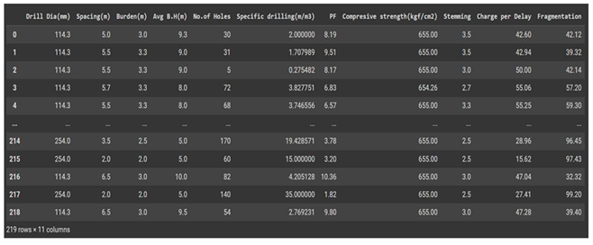
Collecting sample data is the first and most basic step in designing any machine learning or ANN model. It deals with the collection of the right dataset with decided input and output parameters. For the purpose of this paper, secondary data was collected from the blast record of the limestone quarry mining that was used. A number of inputs and output data were collected. In the dataset, there are a total of 219 data points and 11 features. There are a total of 10 input features (Drill Dia (mm), Spacing (m), Burden (m), Average Bench Height (m), Number of Holes, Specific Drilling (m/m3), Powder Factor, Compressive Strength (kgf/cm2), Stemming, and Charge Per Delay) and 1 output feature (Rock Fragmentation).
Table 1.
Visualization Input and output datasets.
Table 1.
Visualization Input and output datasets.
By looking at the data in its raw format, it can be seen that the drill diameter is not changing so much with the changing value of rock fragmentation (most of the time the value is only 114.3). It means it may not be contributing to the variability of our output feature and hence can be eliminated to reduce model complexity. The same is the case with compressive strength. However, we will establish it with the help of a correlation plot and eliminate the unwanted features accordingly.
If we refer to domain knowledge of drilling and blasting in mining, the powder factor in determining rock fragmentation is a very important factor. So, it will contribute significantly to the prediction of rock fragmentation with different models.
Here, the quantity of data is very small, so we will be training both machine learning models (Random Forest Regression (Bagging), Support Vector regression, and XG Boost Regression (Boosting)) as well as a deep learning model (Neural Network Regression) and then assessing the best model for this type of data.
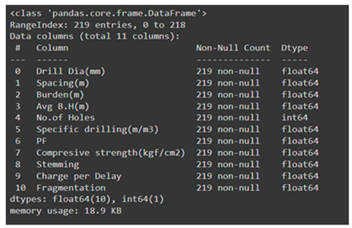
Table 2.
Variable features.
Table 2.
Variable features.
In the dataset, out of 10 input features, 9 have decimal values, and the remaining feature has integer values (number of holes). The output feature, which is rock fragmentation, is also expressed in terms of decimal values.
Since there are no categorical features, there will not be any need to create dummy variables for the purpose of training different models. Also, there will not be any cases of treating imbalanced classes for the same purpose.
4.3,. Pre-processing
Data pre-processing is a technique that involves transforming raw data into a more coherent format. After data collection, the basic data pre-processing procedures are conducted to train the ANNs and MLs more efficiently. The data pre-processing involves checking out missing values, splitting the data into training and test sets, and finally doing feature scaling to limit the range of variables so that they can be compared and worked on in common.
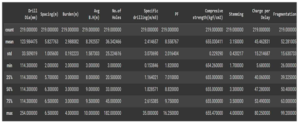
Table 4.
Statistical Parameters.
Table 4.
Statistical Parameters.
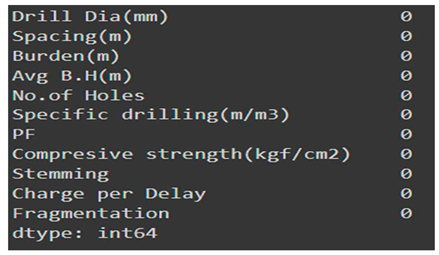
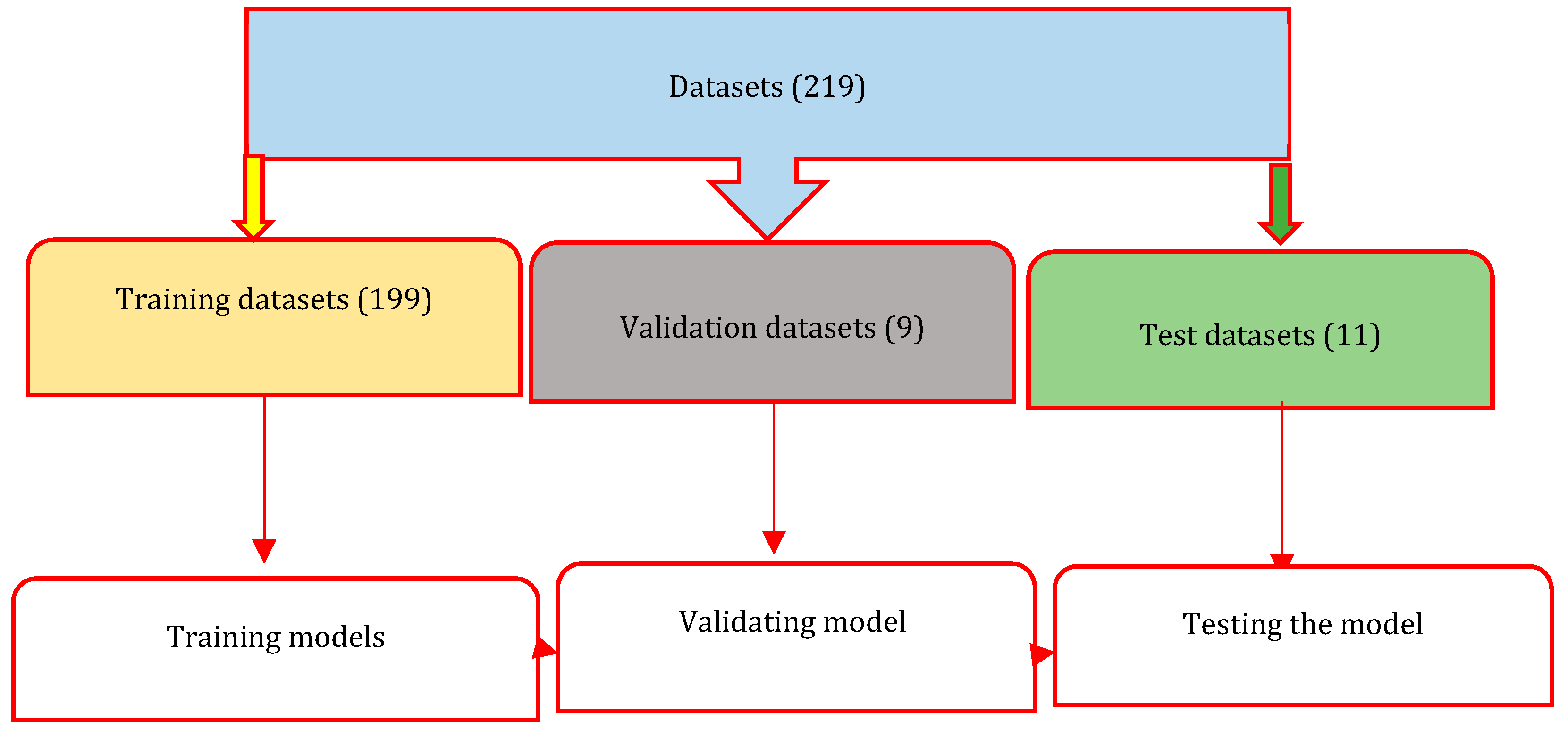
A total of 219 datasets are prepared for the model. As we can see from the table above, there are no missing values for any of our input or output features. Hence, there will not be any need to apply techniques for treating missing values (mean, median, and mode treatment). Afterward, the datasets were grouped into training and testing data sets. 199 data points were considered for training the network, 9 data points (approximately 3.8% of total data) were kept for cross-validation, and 11 data points (approximately 5 % of total data) were considered for testing the model.
4.4. Data Analysis
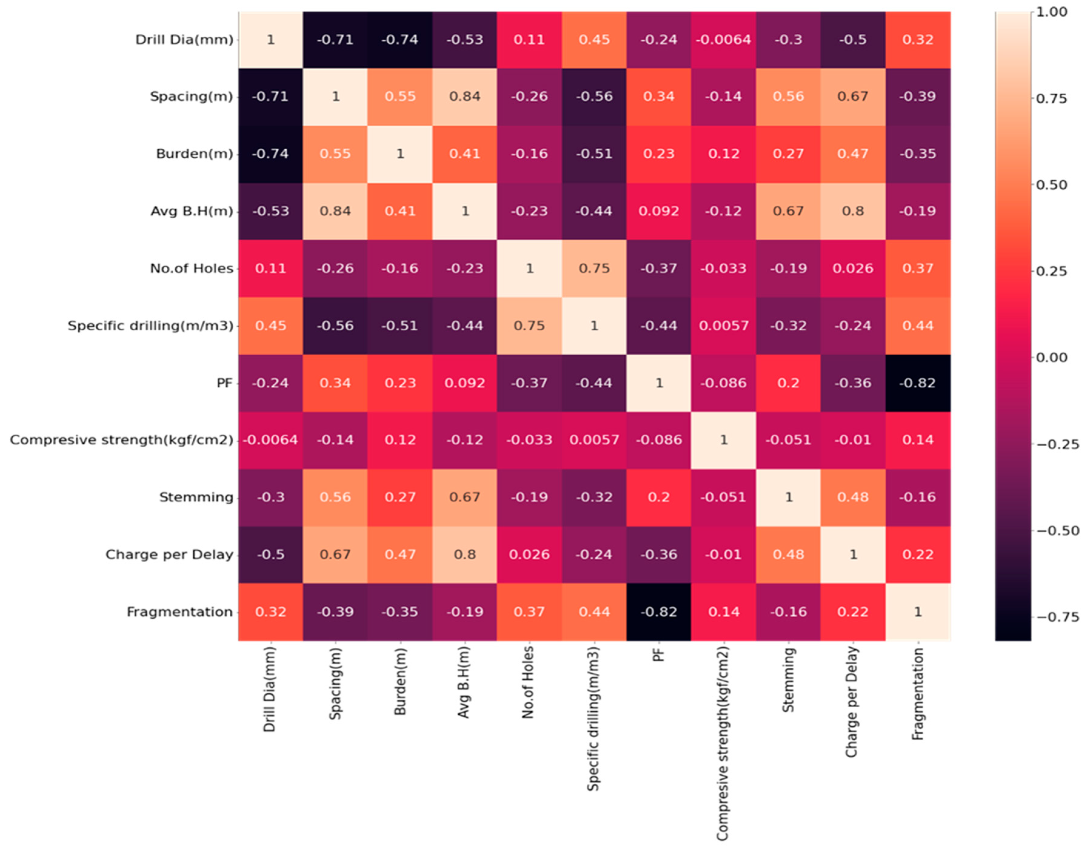
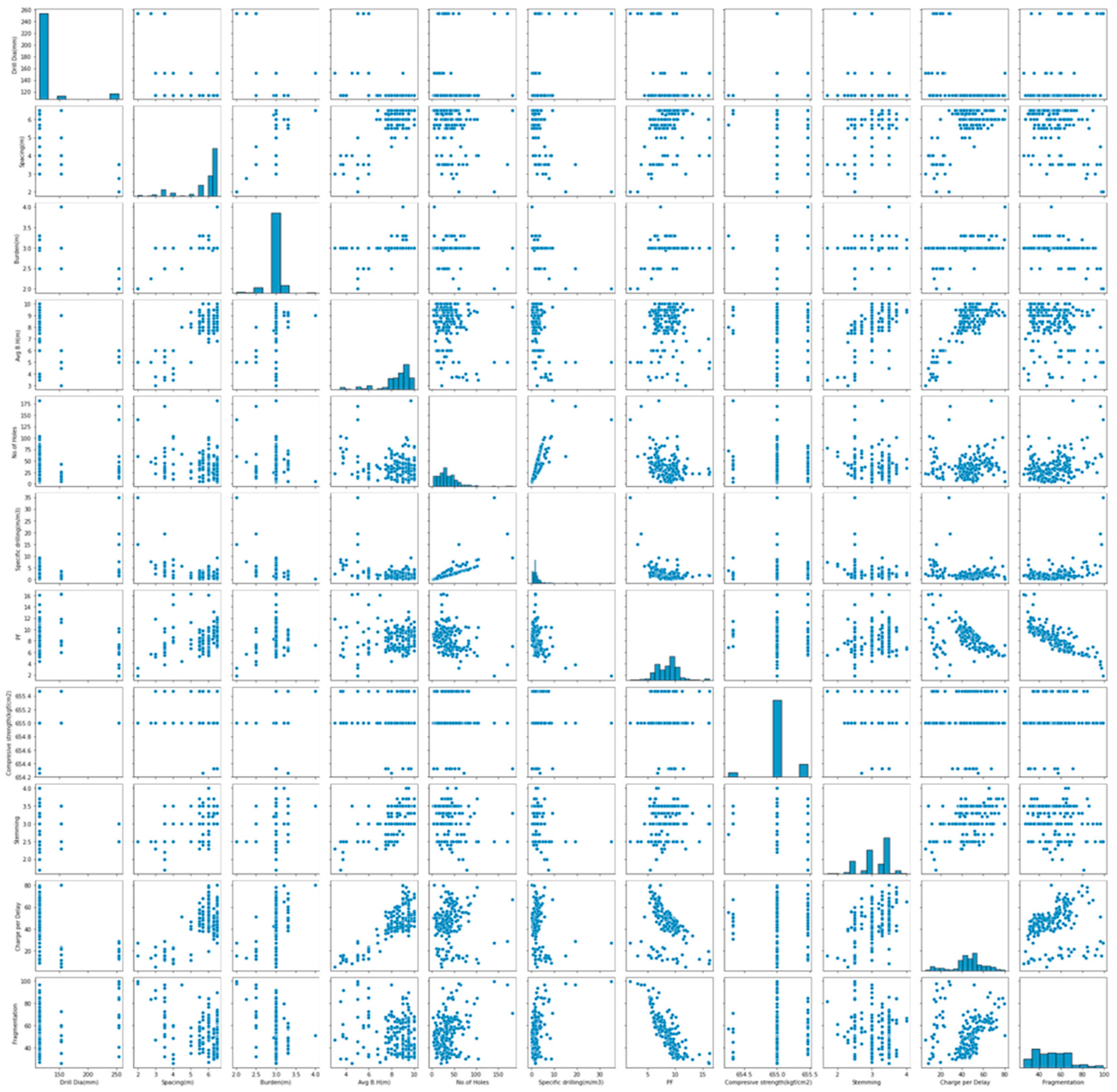
In this study, a total of 11 input parameters (drill hole diameter (mm), spacing (m), burden (m), average bench height (m), number of holes, specific drilling (m/m3), powder factor (PF), compressive strength (kg/cm2), stemming, the charge per delay, and one output fragmentation) are used. The presentation of data in a graphical or pictorial format is known as "data visualization." To get insights, it enables decision-makers to see analytics displayed visually. Visualization action is the act of using visual representations of our data to identify trends and relationships. A variety of Python data visualization libraries, like Matplotlib and Seaborn, are used to do data visualization in this work. Statistical parameters, correlation plots, scatter plots, and histograms are used to visualize and recognize the relationship between the inputs and outputs of the datasets.
Figure 2.
Correlation plot.
Figure 2.
Correlation plot.
Figure 3.
Scatter plots and histograms.
Figure 3.
Scatter plots and histograms.
By looking at the results of the statistical table, correlation plot, and pair plot we can draw the following conclusions:
Drill diameter has a mean of 124 and a standard deviation of 33.5. Its value at the 25, 50, and 75 percentiles is 114.3. It means 114.3 is the most frequently occurring value in it, and this feature may not show any variability with the output feature. Furthermore, its correlation value with rock fragmentation is only 0.32, which means it has a very weak correlation with rock fragmentation and hence cannot contribute anything to the model.
Specific drilling is another such feature that does not show any variability with the output feature as per the statistical description, as well as not showing any sign of a strong correlation with rock fragmentation.
Features like a burden, powder factor, compressive strength, and charge per delay show a normal distribution of their values, which may improve the results of the model by a very small value. Other features are either negatively skewed or positively skewed.
The feature that has the strongest correlation with rock fragmentation is Powder factor (correlation of 0.82). Its value ranges from 1.82 to 16.25 with a mean value of 8.55.
As per the pair plot, the powder factor is also showing a strong decreasing trend with rock fragmentation.
Unlike features like drill diameter, average bench height, compressive strength, stemming, and charge per delay, all other features show strong correlation, so eliminating these weakly correlated features will reduce model complexity.
All of the other features have strong correlations, but drill diameter, average bench height, compressive strength, stemming, and charge per delay don't. Getting rid of these weakly correlated features will make the model simpler.
For training support vector regression, we will need to scale the data as per the standard assumptions of support vector machine-based models. This we can do separately while training the model.
Figure 4.
Splitting of datasets into training datasets, validation datasets, and testing datasets.
Figure 4.
Splitting of datasets into training datasets, validation datasets, and testing datasets.
A feature scaling procedure before presenting the input data to the network is also a good practice since mixing variables with large and small magnitudes will confuse the learning algorithm on the importance of each variable and may force it to finally reject the variable with the smaller magnitude. Normalization is one of the feature scaling techniques in which values are shifted and rescaled so that they end up ranging between 0 and 1. It is also known as Min-Max scaling. The scaling of the input and output parameters is performed using the following equation:
Scaled value = (Unscaled value – Minimum value)/ (Maximum value- Minimum value
4.4. Building the neural network and machine learning model (SVR, RFR, and XG Boost)
We have completed the database with a constrained quantity of data, using the Python programming language to perform multiple machine learning and deep learning methods, and are now going to compare the outcomes of all of them using comparison performance. We chose ANN from deep learning, Random Forest regression, Support Vector Regression, and XG Boost regression from supervised machine learning because each has its strengths that might work for our project.
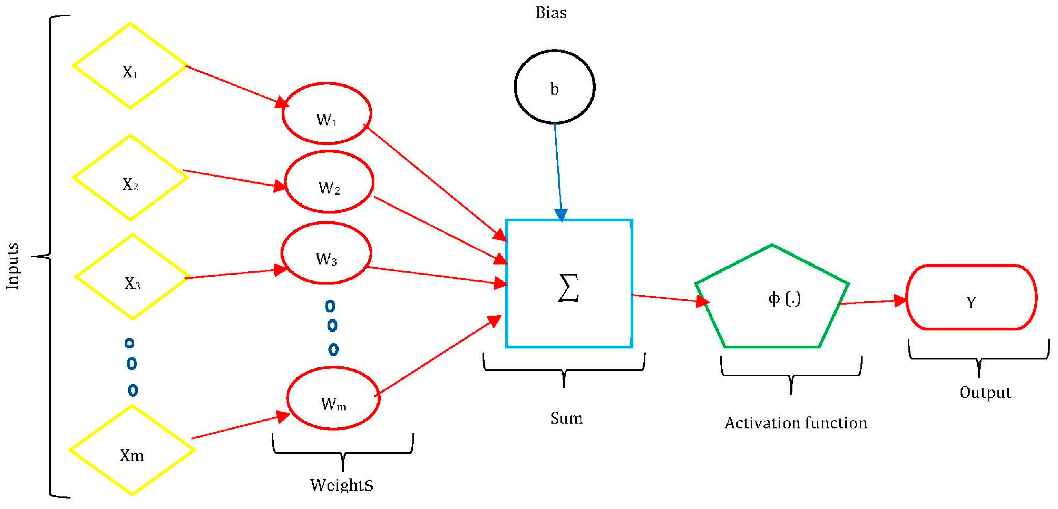
In an artificial neural network model, the number of hidden layers, neurons in each layer, activation function in each layer, training function, weight/bias learning function, and performance function are specified. The input layer contains input neurons (nodes) that send information to the hidden layer. The activation functions in each layer, training function, weight/bias learning function, and performance function are specified. The input layer contains input neurons (nodes) that send information to the hidden layer.
Figure 5.
Artificial neural network structure.
Figure 5.
Artificial neural network structure.
As a supervised learning technique, the random forest has labels for our inputs and outputs as well as mappings between them. It can be used for classification and regression problems [
65]. In the event of regression, the random forest will average the outcomes of each decision tree rather than choosing the vote with the greatest number of participants. For algorithms with large variances, such as decision trees, bagging is a general method that can be used to lower the variance [
66]. Bagging causes each model to run independently before aggregating the results without regard for the performance of any particular model.
The Boost algorithm has been improved by XG Boost [
67]. The trees that minimize a loss function are used to create an XG Boost repressor. A loss function is made up of two components: an error rate that is derived using validation data and a regularization factor to prevent overfitting the model. A scalable end-to-end tree-boosting technique is called XG Boost [
68].
Due to the cost function's disregard for samples whose prediction is close to its target, the support vector regression model can only be created using a portion of the training data. SVR, NuSVR, and LinearSVR are three distinct ways to implement support vector regression. In this paper, for support vector regression, a linear kernel is used.
The following methods are performed in modeling a machine learning model, i.e., Random Forest regression, Support vector regression, and XG Boost regression.
1. Importing Python libraries and loading our data set into a data frame
2. Splitting our data set into a training set and a test set
3. Creating a Random Forest regression, SVR, and XGBR model and fitting it to the training data
4. Visualizing the Random Forest regression, SVR, and XGBR results.
4.5. Sensitivity analysis
Sensitivity analysis was used to assess the effects of different blasting parameters on fragmentation by determining how different parameters affected the way rocks broke apart [
69]. To solve this issue, the Shapley effects were recently developed. They divide the mutual contribution of a group of inputs (owing to correlation and interaction) among all of the inputs in the group [
70]. Permutation importance and shapely values are used as feature importance measures to identify the sensitivity analysis in this work.
The Shapley value is a tool used in machine learning for data valuation, ensemble pruning, multi-agent reinforcement learning, explainability, and feature selection [
71]. [
72] stated that the Shapley value has been used as the foundation for many techniques that link a machine-learning model's predictions on input to its underlying features. A model-independent global explanation technique that sheds light on a machine learning model's behaviour is feature permutation importance. Depending on how each feature affects the predictions made by the machine learning model that has been trained, it calculates and ranks the relevance of each feature.
3. Results and Discussion
Model
Using the correlation plot shown in
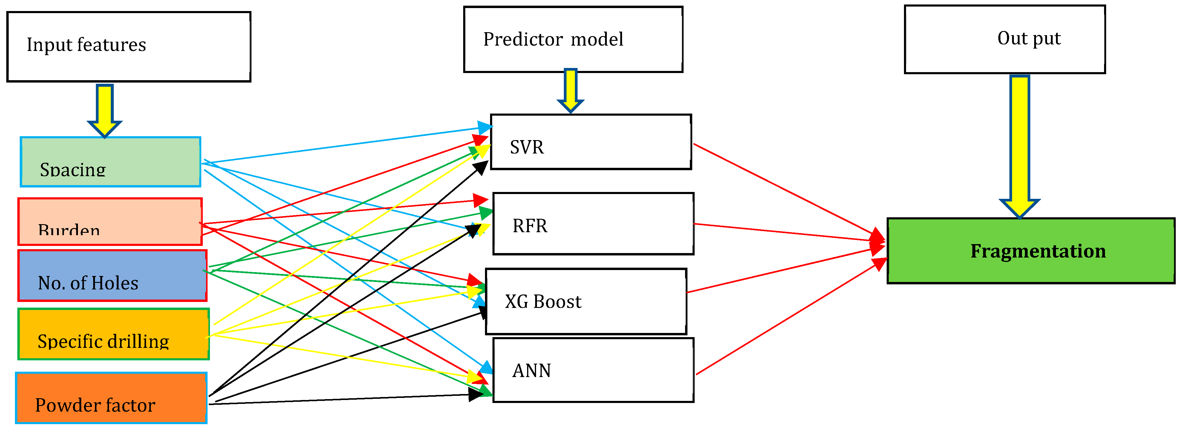
Figure 2, we have seen the relationship between different input parameters and the output parameter, which is fragmentation. Some of the input features (drill diameter, average bench height, compressive strength, stemming, and charge per delay) showed a weak correlation with rock fragmentation. To reduce model complexity, we eliminated those weakly correlated parameters are eliminated in all models we trained.
Figure 6.
Input parameters and models used for predicting fragmentation.
Figure 6.
Input parameters and models used for predicting fragmentation.
Mean absolute error (MAE), mean absolute percentage error (MAPE), mean square error (MSE), root mean square error (RMSE), and determination coefficient (R2) is used to compare the performance of the machine learning analysis and ANN approach models.
1, Results of Random Forest Regression (RFR)
• Model parameters: estimators = 10
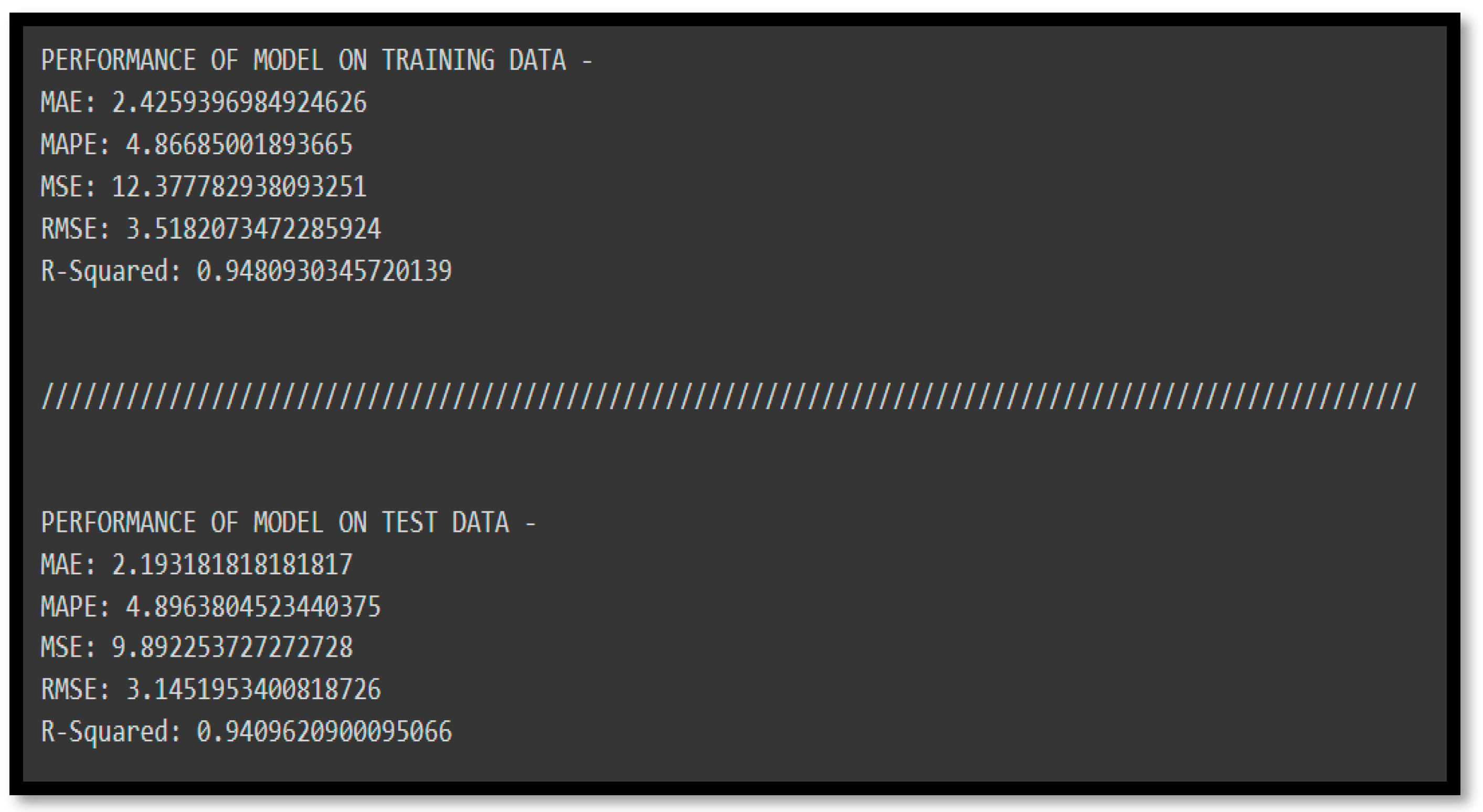
Figure 7.
Performance model of Random Forest Regression (RFR).
Figure 7.
Performance model of Random Forest Regression (RFR).
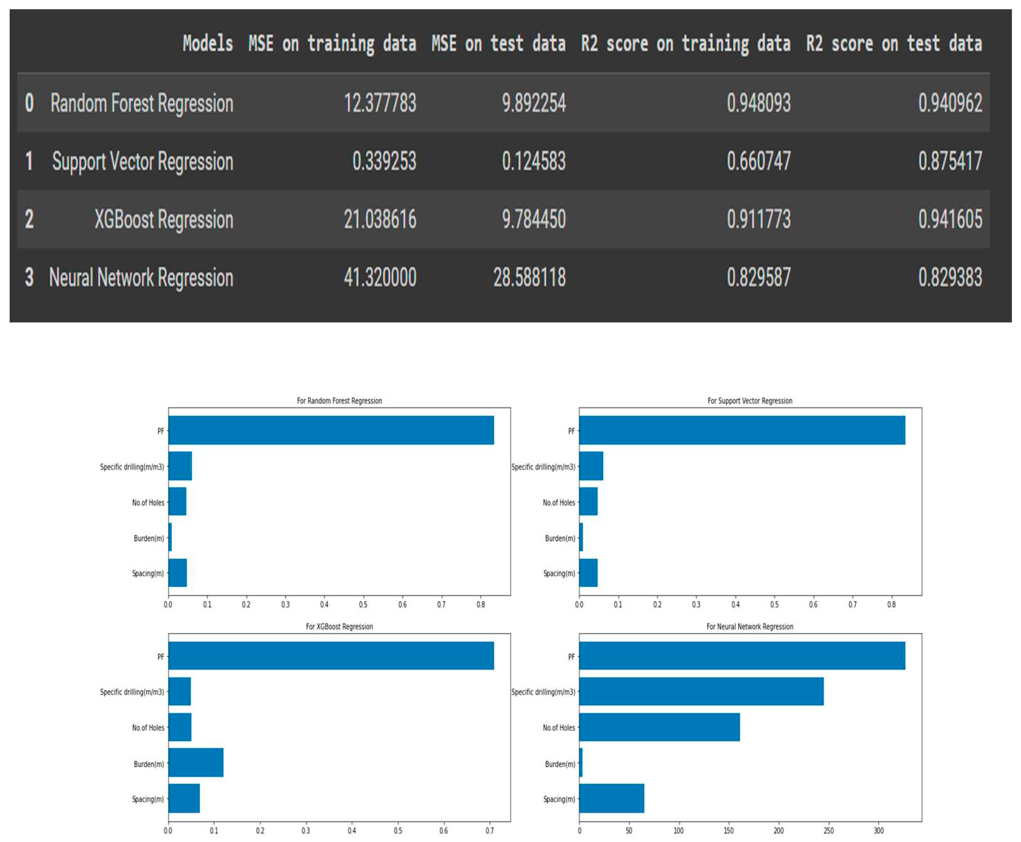
The mean squared error values for training and test data are 12.37 and 9.89. Similarly, the R2 value for both the training and test data is 94%. It means there is no issue of underfitting or overfitting with this model. It also means that random forest regression has the potential to perform well on this kind of data (from varied distributions).
The mean squared error values for training and test data are 12.37 and 9.89. Similarly, the R2 value for both the training and test data is 94%. It means there is no issue of underfitting or overfitting with this model. It also means that random forest regression has the potential to perform well on this kind of data (from varied distributions).
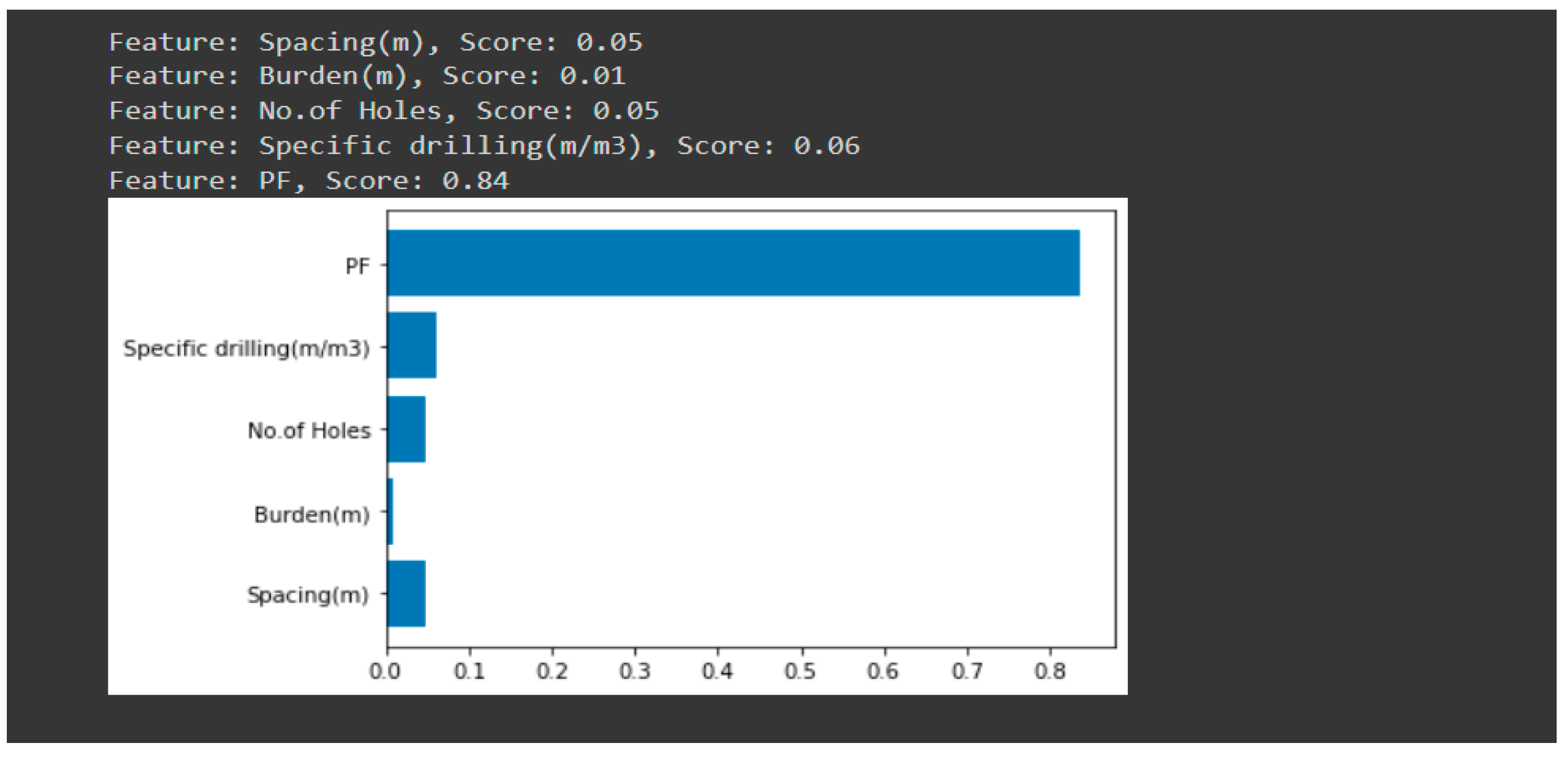
Figure 8.
Feature importance of the Random Forest Regression (RFR) model.
Figure 8.
Feature importance of the Random Forest Regression (RFR) model.
According to the feature importance figure from the random forest regression model, the powder factor is the most important feature and the burden is the least important feature in the determination of rock fragmentation. All other features are not as significant as the powder factor and have a score of 0.8 less on the feature importance scale.
2, Results of Support Vector Regression (SVR)
Figure 9.
Performance model of Support vector regression (SVR).
Figure 9.
Performance model of Support vector regression (SVR).
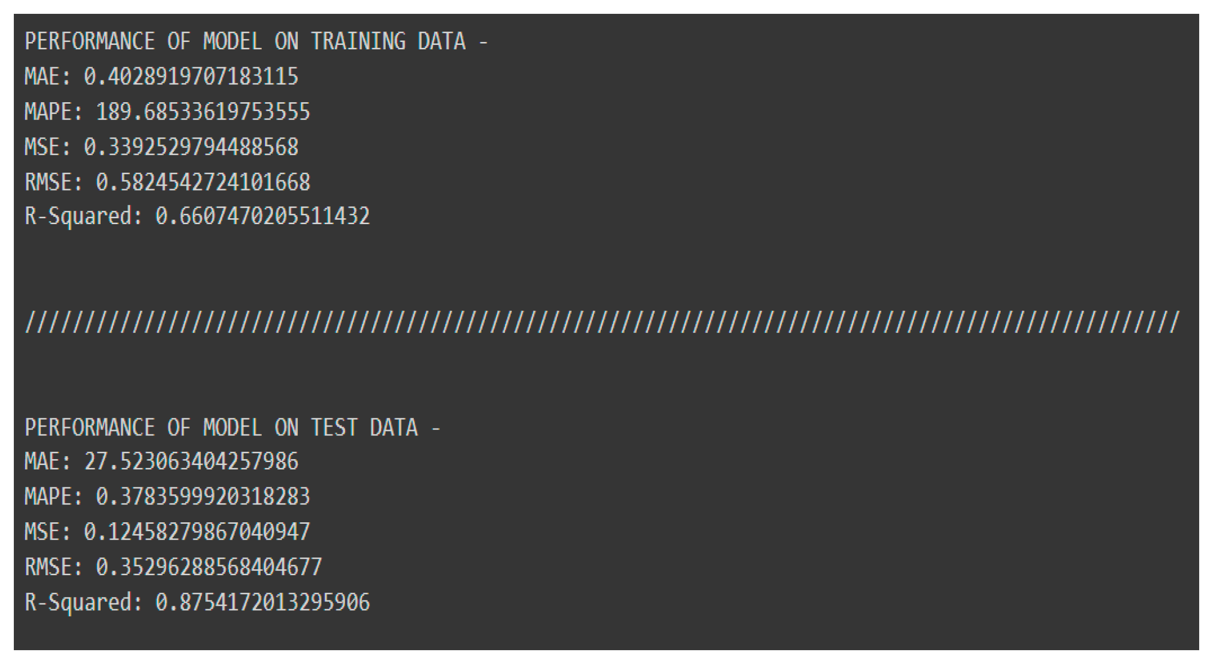
The above figure shows the mean squared error values for both training and test data are 0.339 and 0.124, respectively, which seem small because of data scaling. Similarly, the R2 values for both the training and test data are 66% and 87%, respectively. With this model, there is an issue with over- and under-fitting. Because the variability of training data is low, this model was unable to investigate the variance between input features and output features. Also, it is showing that support vector regression has no potential to perform on this kind of data (from varied distributions).
Figure 10.
Feature importance of the Support vector regression (SVR) model.
Figure 10.
Feature importance of the Support vector regression (SVR) model.
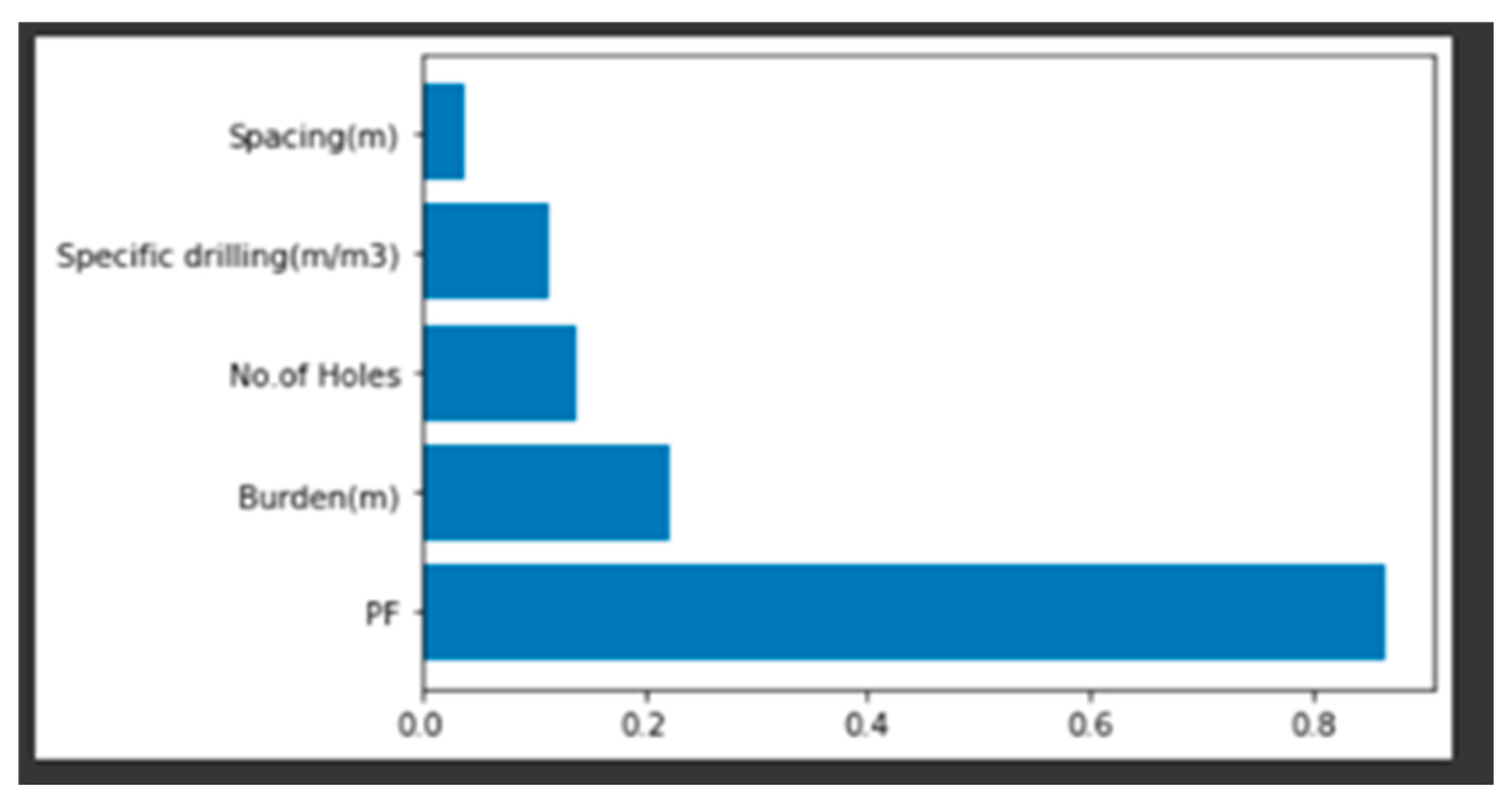
According to the feature importance figure from the support vector regression model, the powder factor is the most important feature, but instead of being a burden, spacing is the least important feature in the determination of rock fragmentation. All other features are showing more significance as compared to what we have in the random forest regression model. This is happening because of the bad fit of the SVR on the dataset.
3. Results of XG Boost Regression (XGBR)
Figure 11.
Performance model of XG Boost regression.
Figure 11.
Performance model of XG Boost regression.
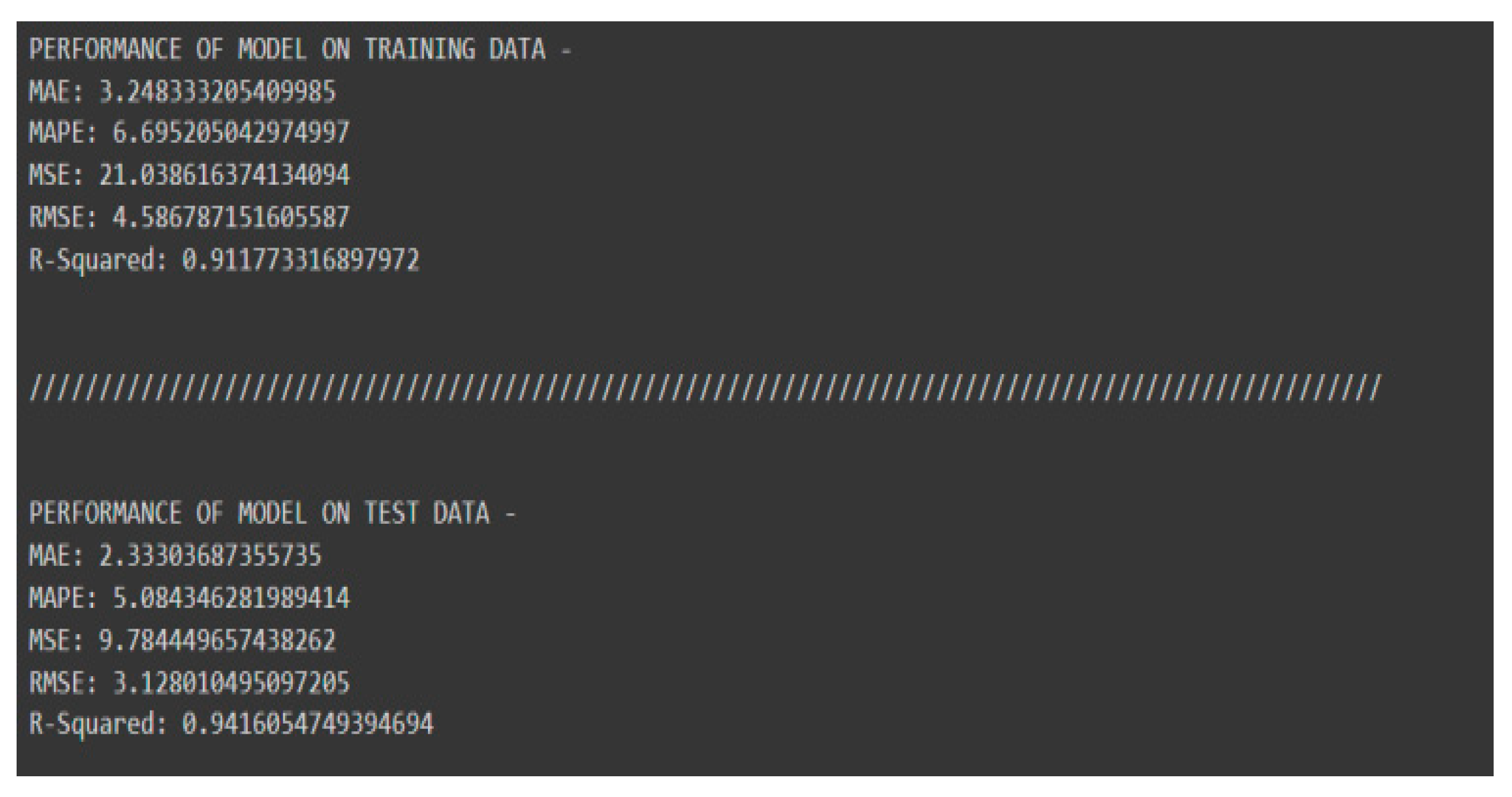
The mean squared error values for both training and test data are 21.03 and 9.78, respectively, which is a little bit more than what we have in the RFR model. Similarly, the R2 values for both the training and test data are 91% and 94%, respectively.
Since the difference between the two is significant, we are probably underfitting this model, i.e., not being able to study the variability of input variables with the output variable.
It shows that XG boost regression has the potential to perform on this kind of data (from varied distributions), but we need more data for better performance.
Figure 12.
Feature importance of XG Boost regression model.
Figure 12.
Feature importance of XG Boost regression model.
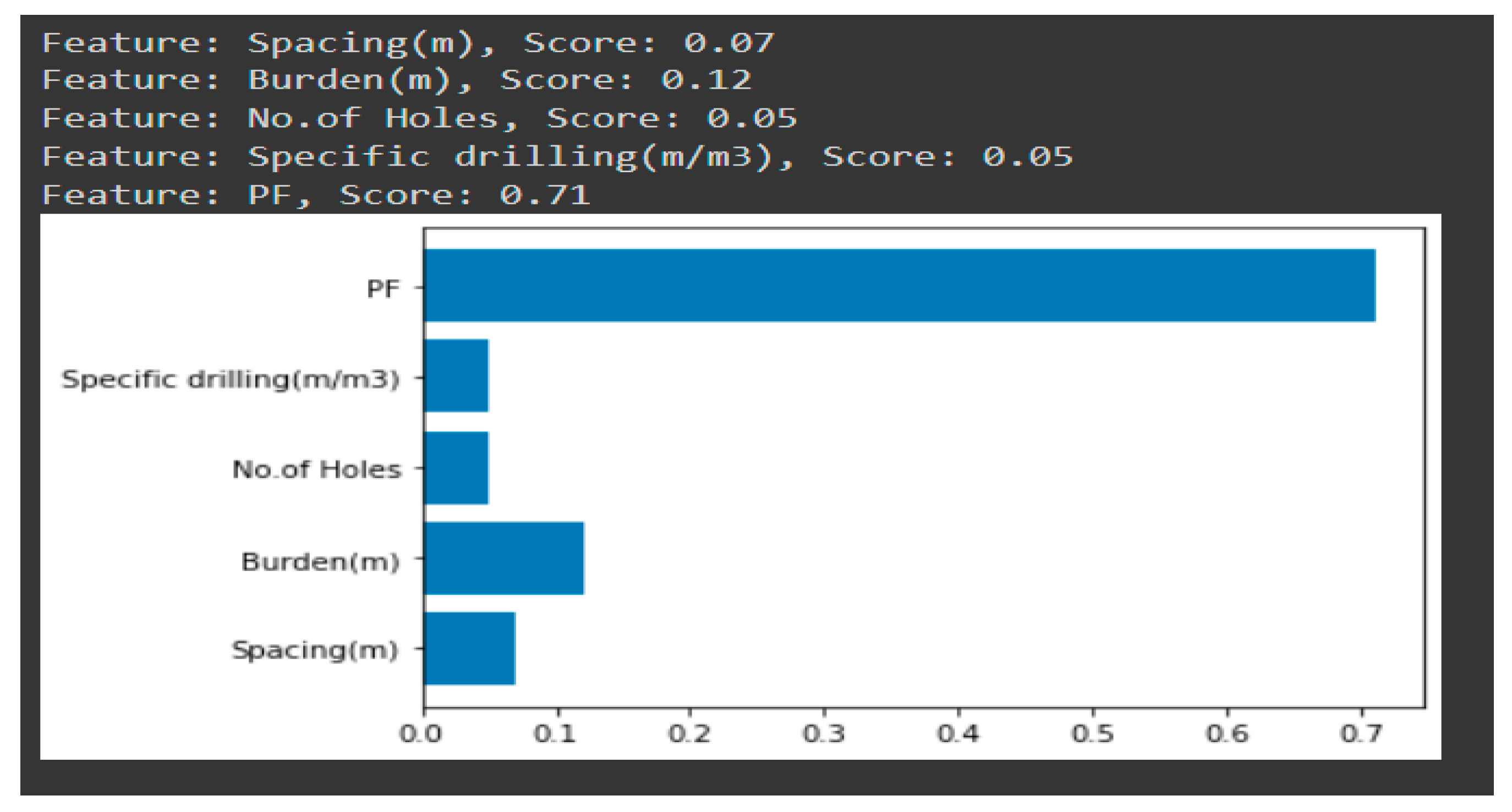
features are showing more or less the same significance as compared to what we have in the random forest regression model.
This is again happening because of the bad fit of the XG boost regression on the dataset.
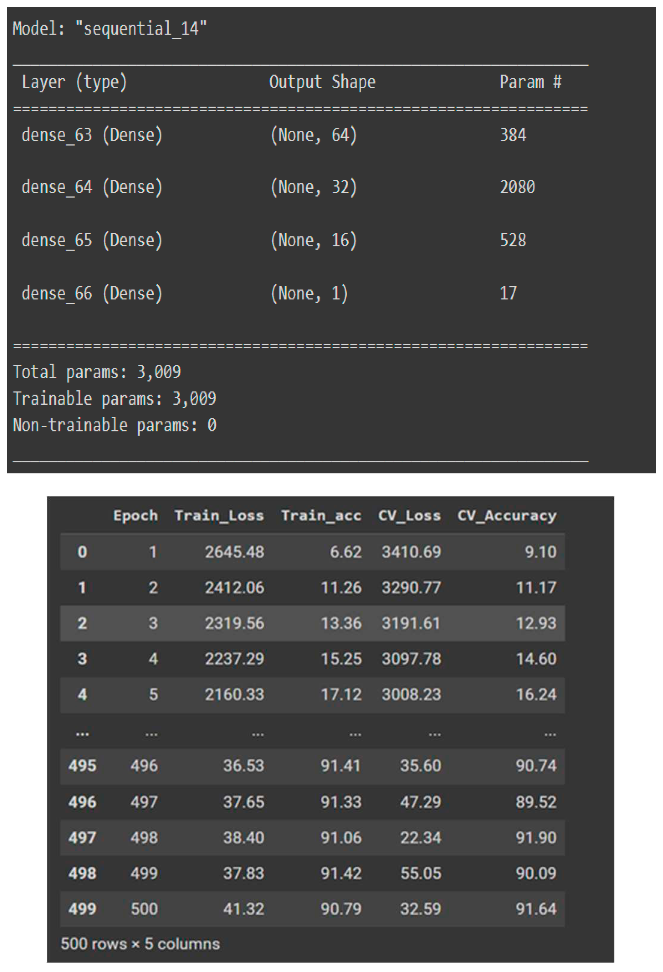
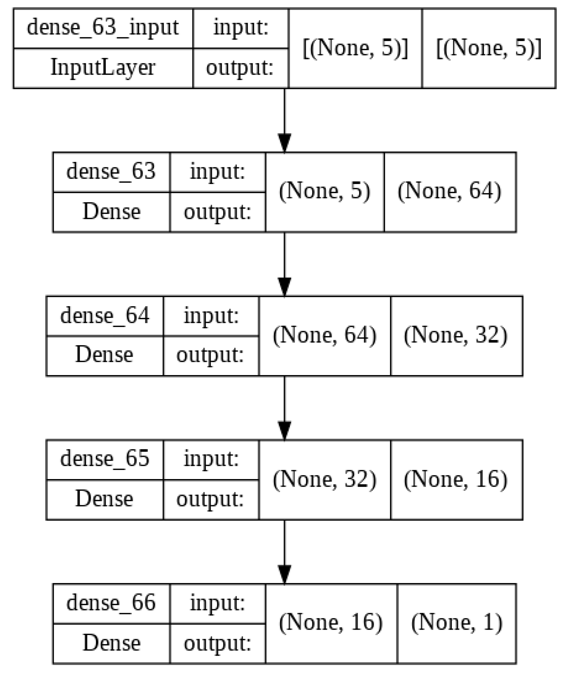
3. Results of Artificial neural network (ANN)
Structure of the neural network
Figure 13.
Structure of the neural network model developed.
Figure 13.
Structure of the neural network model developed.
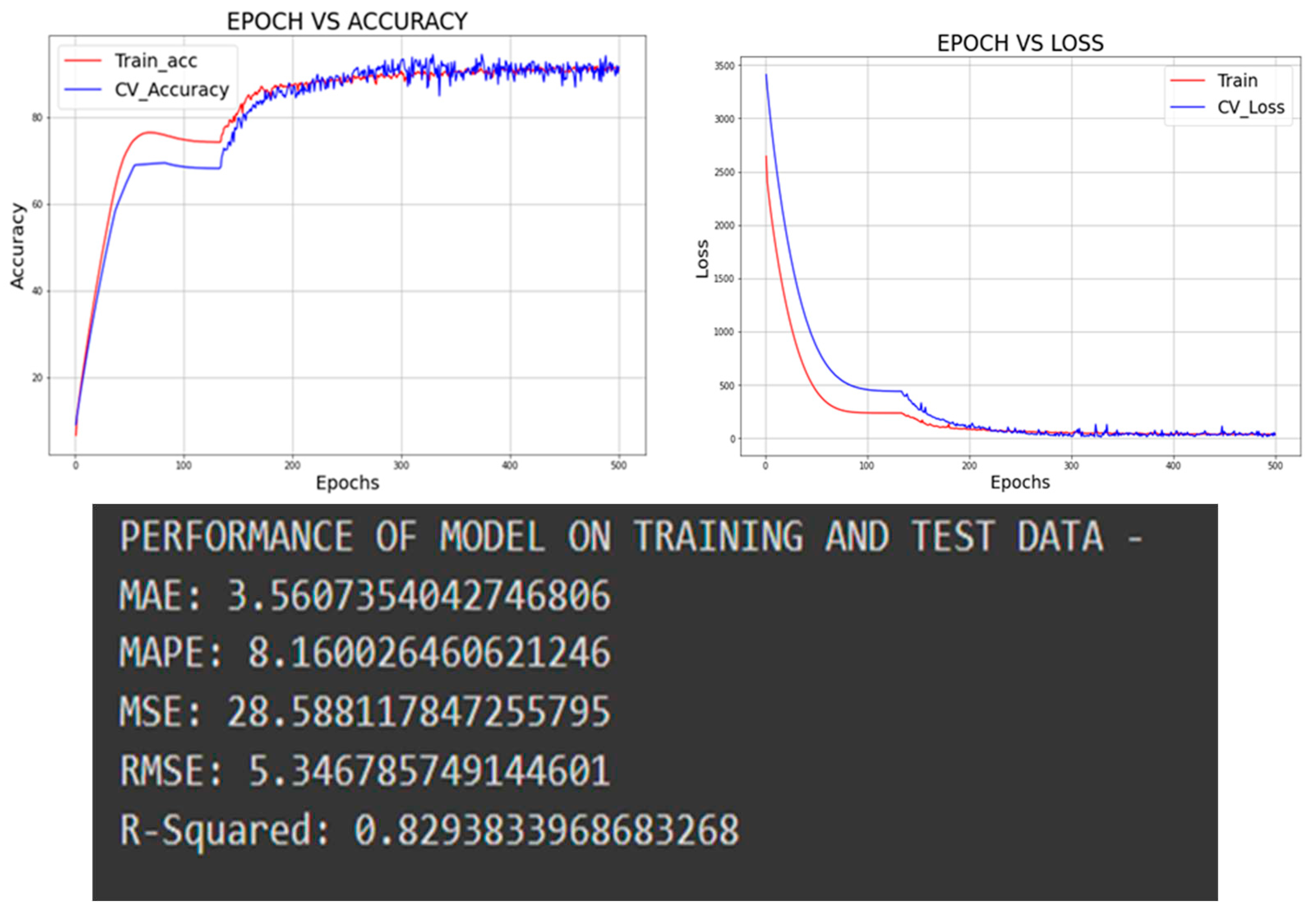
Figure 14.
Performance model of ANN on training and test data .
Figure 14.
Performance model of ANN on training and test data .
The mean squared error values for training and test data are 41.31 and 28.58, respectively. Similarly, the R² value for both training and test data is near 83%. It means that there is no issue of underfitting or overfitting with this model. The performance of the model can still be improved if we get more data, but it is also not giving any unrealistic figures, as we were getting in the case of the random forest regression model.
It is showing that neural network has the greatest potential for performing on this kind of data (from varied distributions) if collected in large quantities.
A. Feature Importance
Now, which of the explanatory variables is most relevant when predicting the fragmentation percentage? This is a very important question. This question is almost as old as the field of statistics itself. When it comes to linear models and other “white-box” approaches, the straightforward answer is given in traditional statistical books. What happens when the model is not as interpretable as a simple linear model? It is now not enough to look at the coefficients themselves. Instead, we make use of the computation power of our computers and calculate the so-called permutation importance.
The intuition behind permutation importance is straightforward. The only requirement is to have fitted a model, either for regression or classification. If a feature is deemed unimportant by the model, we can shuffle it (rearrange the rows) with little effect on the model's performance. On the other hand, if the feature is relevant, shuffling its rows will negatively affect the prediction accuracy.
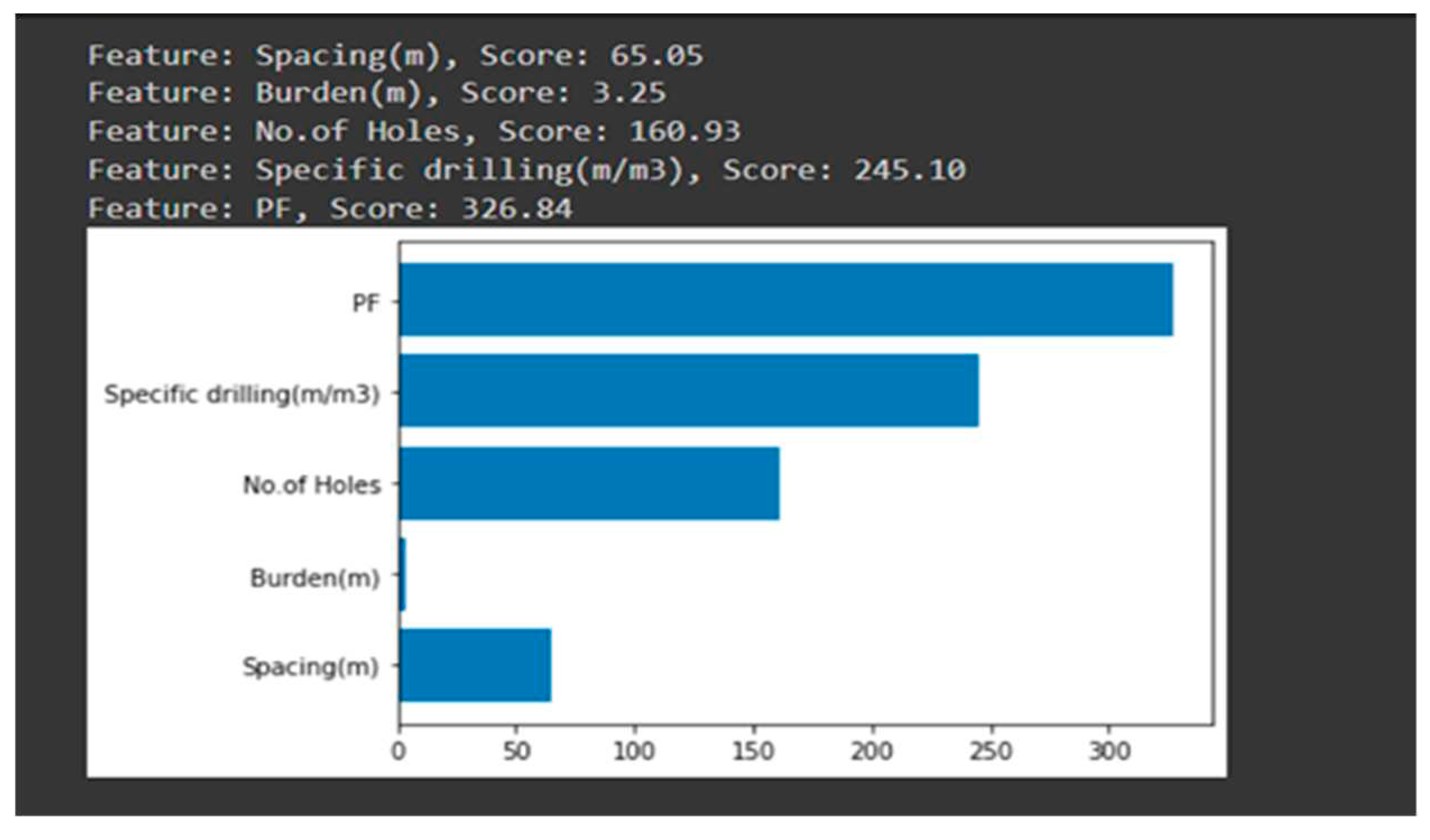
Figure 15.
Feature importance of ANN model.
Figure 15.
Feature importance of ANN model.
According to the feature importance of the neural network model (figure 15), the powder factor is the most important feature in the RFR, SVR, and XGBR models. The burden is the least important feature in the determination of rock fragmentation, as we were getting in the RFR model. Other features are showing more significance as compared to what we have in other models.
B. Residual plots
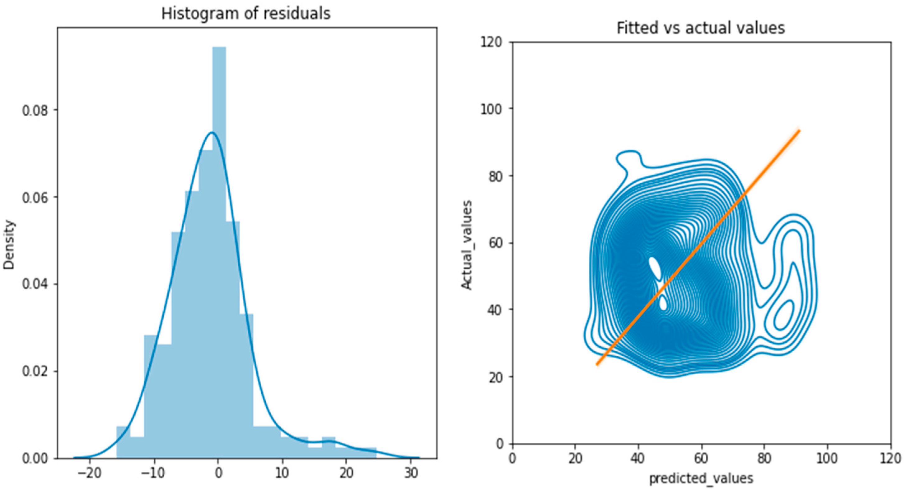
Figure 16.
Residual plots.
Figure 16.
Residual plots.
There is nothing too strange, and the model is behaving as it should according to the terms of NN concepts. There are several points one can explore here, like:
According to the histogram generated above, residuals are following a normal distribution with a mean of 0. It means the residuals satisfy the constant variance assumption for the unbiasedness of ordinary least squares estimators (mean squared error) and show that selected features are optimal for the prediction of rock fragmentation.
The second graph is a kernel density estimate (KDE) plot, which is a method for visualizing the distribution of actual and predicted values, analogous to a histogram. It is showing that the predicted values of rock fragmentation are in line with the actual values of the same. The range covered is 25 to 100 for predicted values and 25 to 90 for corresponding actual values. The central tendency for both values is near 45 which depicts that model is giving the same statistical observations as the actual rock fragmentation value for the predicted rock fragmentation value.
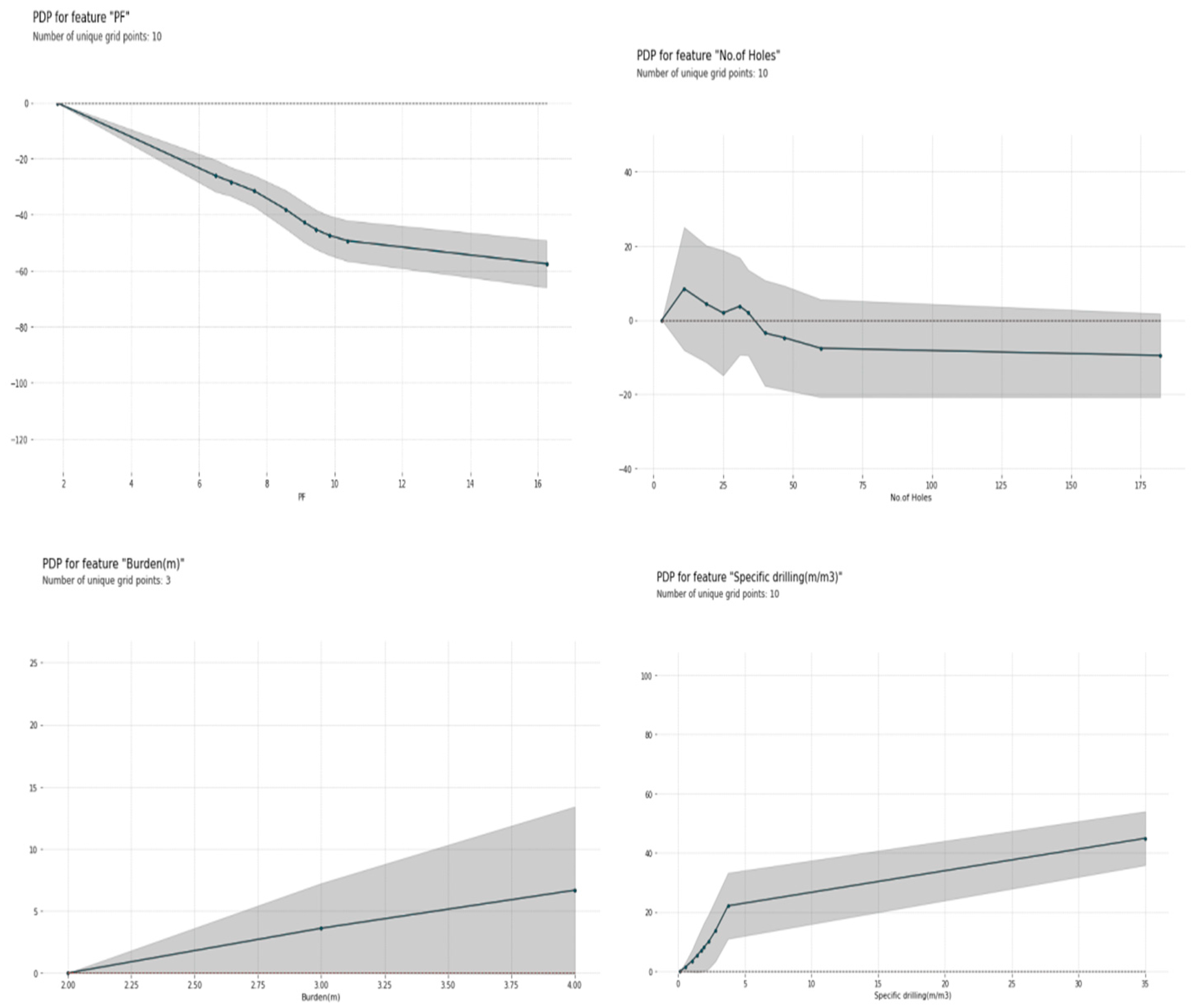
C. Partial dependence plots
Permutation importance allowed us to find out which variables are most important in terms of predicting rock fragmentation. The next question comes naturally: What is the effect of such variables on the value of rock fragmentation? In the world of linear models, this question is answered by looking at the coefficients. In the black-box world, we look at the partial dependence plots (PDP).
The underlying idea behind these plots is to marginalize the effect of one or two variables over the predicted values. When a neural network has several features and layers, it is really hard or even impossible to assess the impact of a single feature on the outcome by simply looking at the coefficients. Instead, the marginal effect is approximated by a Monte Carlo approach. We run predictions for a set of features and then average them out over the features for which we are interested in knowing their effects.
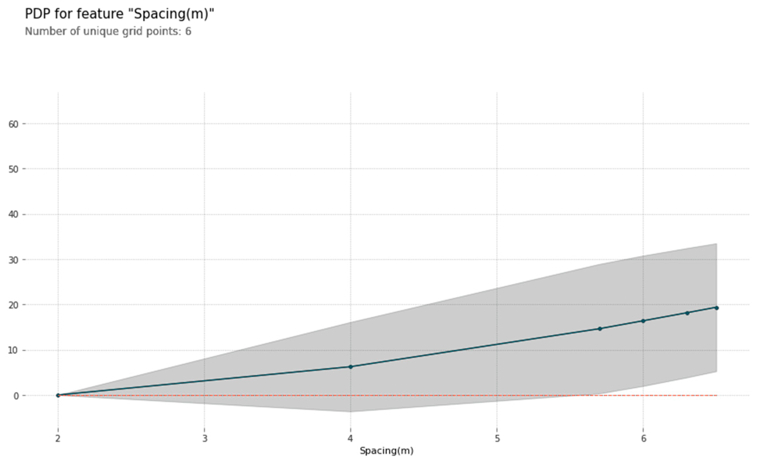
From the following figures, we can draw some interesting conclusions:
1, Higher values of spacing, burden, and specific drilling lead to higher values of rock fragmentation.
2, The change in the number of holes has a negligible impact in the range of more than 40 holes. There are some cases (number of holes less than 40) where the relationship with rock fragmentation is positive. It means the effect of the number of holes on rock fragmentation stabilizes after a value of 40.
3, The powder factor has a decreasing effect on the value of rock fragmentation with its increasing value which was also confirmed earlier with a correlation plot.
Figure 17.
Partial dependence plot.
Figure 17.
Partial dependence plot.
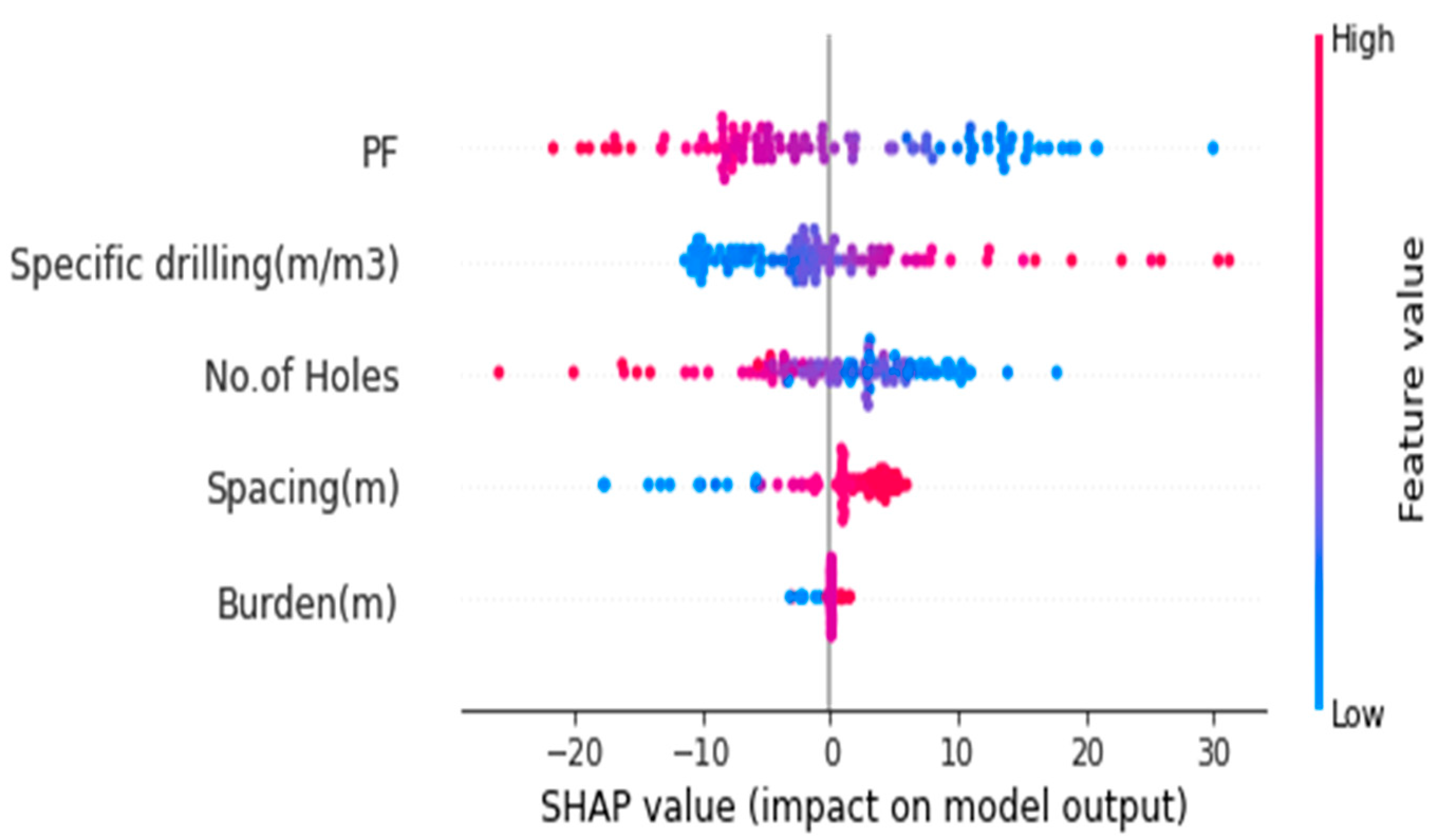
D, Shapely values
Shapely values contribute to understanding the model in an analogous way to coefficients in a linear model. Given a prediction, how much of it is affected by the explanatory variables? What features contribute positively and negatively?
The Shapley value is the average marginal contribution of a feature value over all possible combinations of the other features. They are useful for understanding the contributions of the features of the model when we produce a prediction. Shapely values answer "why" the prediction is different from the mean prediction.
Figure 18.
shapely values.
Figure 18.
shapely values.
Each row corresponds to a feature, the color represents the feature value (red high, blue low), and each dot corresponds to a training sample.
From the combined Shapely plot values, we observe the following:
1, Powder factor is the feature with the highest impact. We already found this out when calculating the permutation importance. Nevertheless, it is always a good idea to double-check our conclusions. The effect of specific drilling is reversed to the powder factor: higher specific drilling levels imply more rock fragmentation.
2, Burden and spacing seem somewhat irrelevant because the least impact is there for these features than the value of powder factor. They may also be removed from the model.
5, Combined Support Vector Regression, Random Forest Regression, XG Boost Regression ANN results
Table 6: combined Support Vector Regression, Random Forest Regression, XG Boost Regression, and ANN Accuracies result
Figure 19.
Importance figure of Combined Support Vector Regression, Random Forest Regression, XG Boost Regression ANN results.
Figure 19.
Importance figure of Combined Support Vector Regression, Random Forest Regression, XG Boost Regression ANN results.
