3.1. Pearson Correlation Coefficient
The statistics of each measurement variable are shown in
Table 3 and
Table 4. The initial investigation relied on simple correlation analysis (
Table 5) due to the variance in measurement units between water quality parameters and biometric parameters. The standardized correlation coefficient (r) is utilized to evaluate the level of linear correlation between each measurement variable and is employed as a benchmark for the development and refinement of subsequent models.
The standardized correlation coefficient (r) ranges between -1 and +1, with a value closer to -1 or +1 indicating a stronger correlation between the two random variables, and a value closer to 0 indicating a weaker correlation. In
Table 5, it is evident that a majority of the measurement variables under investigation in this study exhibit a substantial degree of linear relationship, while the remaining variables cannot be determined as having a linear relationship (potentially due to a non-linear relationship or lack of correlation).
As correlation analysis only reveals the existence of linear relationships between variables, it does not imply the establishment of a causal relationship. Thus, in order to identify any potential variables and investigate the common variance between each variable, further factor analysis must be conducted.
3.2. Factor Analysis of Environmental Variables
Before conducting factor analysis, it is necessary to determine the suitability of each measurement variable by checking if the Kaiser-Meyer-Olkin (KMO) value is greater than 0.6 and if Bartlett's sphericity test is significant (p ≦ 0.05). This study hypothesizes that environmental variables, such as nitrate, silicate, phosphate, nitrite, temperature, salinity, pH, dissolved oxygen, transparency, and chlorophyll a, have effects on biological variables, such as the number of zooplankton, crab larvae, shrimp larvae, fish eggs, larvae, fish species, and fish abundance. Therefore, potential factors were first extracted from all the environmental and biological variables. Among the observed variables related to phytoplankton, only the "number of phytoplankton" was included in the analysis of biological variables as it can explain the variation in phytoplankton community structure, hence it is reserved in the SEM but excluded from factor analysis of the biological variables.
3.2.1. First Factor Analysis
The result of the first factor analysis of the environmental variables indicated a KMO value of 0.642. As per Kaiser's suggested criteria, a value between 0.6 and 0.7 is considered to have "normal" applicability. Furthermore, Bartlett's sphericity test was significant (p<0.001), implying that the water quality measurement variables investigated in this study are appropriate for factor analysis.
In this study, the principal component method of extraction was employed to extract factors. Following Kaiser's Criterion, only factors with eigenvalues greater than or equal to 1 were retained. The scree plot was also used to observe the slope of the cumulative explanatory power. When the slope is significantly flattened, the extraction process can be stopped. The results indicated that three factors have eigenvalues greater than 1 and can explain 61.075% of the total variation. With the determined principal components, factor rotation was then conducted.
The purpose of factor rotation is to make the data conform to the assumptions of the statistical model and to convert the data. By rotating the axis in the “maximum space covering range”, associated with different factor loading to increase the differences. In other words, it sets to achieve the greatest amount of variation. Through rotation, both positive and negative correlations between each factor (axis) and variables are strengthened, thus variables that were initially relevant will maintain a high factor loading, which is conducive to naming and interpreting the factors (latent variable).
In this study, the varimax method of orthogonal rotation made each variable have only one factor producing a large factor loading and avoiding duplication. The orthogonal rotations allow the axes to maintain a 90-degree angle, and the varimax method allows a set of variables with high factor loading and the rest with low factor loading, making the factor easy to interpret.
Ensuring construct validity, which refers to the degree to which a measurement variable effectively captures the abstract concept it's intended to measure, necessitates that all elements of the variable exhibit both convergent and discriminant validity. Convergence validity refers to the degree to which variables on the same factor component axis correlate with each other. Additionally, a variable that can be assigned to multiple factors simultaneously does not demonstrate discriminant validity, which refers to the degree to which variables on different factor axes correlate with each other.
After rotation, factor 1 (nitrate, silicate, phosphate, nitrite) can explain 24.528% of the variance; factor 2 (temperature, dissolved oxygen, salinity) can explain 18.505% of the variance; factor 3 (transparency, chlorophyll a) can explain 18.042% of the variance. The findings of the study indicated that the pH environmental variable did not demonstrate adequate convergence validity in the construct validity, as none of the three different rotations produced factor loading values above 0.5.
Communality is a measure that indicates the extent to which a variable contributes to a factor. It ranges from 0 to 1, with higher values indicating that the variable is more closely related to the common factor and has lower uniqueness. Thus, a variable with higher communality is considered a more appropriate measurement variable. The communality of pH is 0.359, the lowest value among all measurement variables. According to Chen (2005), a factor loading of greater than 0.5 and a communality of greater than 0.5 are significant criteria [
13]. Therefore, since pH does not have convergent validity, it has been removed, and a second factor analysis was conducted. Note that when deleting variables, it is essential to remove only one at a time and consider the importance of each variable to the research.
3.2.2. Second Factor Analysis
The second attempt resulted in a KMO value of 0.632 indicating normal applicability. Additionally, Bartlett’s sphericity test was significant with p < 0.001. The results showed that after removing pH, the remaining environmental variables are still suitable for factor analysis.
In the second step, the scree plot diagram revealed that three factors had eigenvalues greater than 1, resulting in a cumulative total variation of 65.360%. These factors were further processed in factor rotation.
After the rotation, factor 1 (nitrate, silicate, phosphate, nitrite) can explain 25.860% of the variance; Factor 2 (temperature, dissolved oxygen, salinity) can explain 20.347% of the variance; factor 3 (chlorophyll a, transparency) can explain 19.153% of the variance. It is evident that the "salinity" environmental variables can be observed in both factor composition axes 2 and 3, with both exceeding a factor loading of 0.5. This indicated that salinity lacks discriminant validity. However, none of the other environmental variables from factors 1 to 3 exhibited factor loadings of 0.5 and above simultaneously, implying that these variables possessed discriminant validity. Moreover, none of the environmental variables in factors 1 to 3 have all factor loadings below 0.5, indicating that variables from factor 1 to 3 possessed convergent validity. Lastly, it is essential to examine whether the communality of the environmental variables is greater than or equal to 0.5. As illustrated in
Table 7, "nitrite" exhibits a communality of 0.427, which is lower than 0.5, rendering it the smallest of the other environmental variables. Therefore, it was eliminated, and the third factor analysis was executed.
3.2.3. Third Factor Analysis
The third factor analysis yielded a KMO value of 0.579 which is deemed as "not a good fit". However, Bartlett's sphericity test was significant (p<0.001), indicating the presence of sufficient correlation among the variables. Nonetheless, given the low effect of extracting common factors as revealed by KMO, it is not advisable to proceed with further analysis of the remaining environmental variables if nitrite is eliminated.
The sea area of the present study exists interrelationships among various water quality environmental measurement variables. Specifically, the study examined the relationship between phosphate and nitrate, which serve as raw materials for the synthesis of organic matter by photosynthesis of marine plants, and silicates, which are the primary constituent materials of phytoplankton cell wall. These interrelationships arise from the interaction between environmental and biological variables. However, given the dynamic nature of marine environments, it was challenging to identify the precise nature of these relationships. Furthermore, deleting any variable may result in interpretational errors. Hence, the researchers chose to exclude only the pH variable. The remaining environmental variables were retained and named based on the outcomes of the second factor analysis as shown in
Table 6 and
Table 7.
Table 6.
The component matrix of environmental variables in each factor after rotation (pH excluded).
Table 6.
The component matrix of environmental variables in each factor after rotation (pH excluded).
| measured variable |
factor loading(N=223) |
| 1 |
2 |
3 |
| nitrate |
0.828 |
0.191 |
-0.019 |
| silicate |
0.811 |
-0.113 |
0.084 |
| phosphate |
0.693 |
0.090 |
0.193 |
| nitrite |
0.584 |
0.290 |
-0.053 |
| temperature |
-0.297 |
-0.836 |
0.051 |
| dissolved oxygen |
-0.082 |
0.737 |
0.428 |
| salinity |
0.198 |
0.639 |
-0.563 |
| chlorophyll a |
0.158 |
-0.088 |
0.777 |
| transparency |
-0.066 |
-0.180 |
0.754 |
| eigenvalue |
2.237 |
1.831 |
1.724 |
| variance % |
25.860 |
20.347 |
19.153 |
| cumulated variance % |
25.860 |
46.207 |
65.360 |
Table 7.
The communality of environmental variables (pH excluded).
Table 7.
The communality of environmental variables (pH excluded).
| environmental variables |
total variance extracted % |
| temperature |
.789 |
| salinity |
.765 |
| dissolved oxygen |
.733 |
| transparency |
.606 |
| chlorophyll a |
.637 |
| nitrate |
.722 |
| nitrite |
.427 |
| phosphate |
.525 |
| silicate |
.678 |
3.2.4. Factor Naming
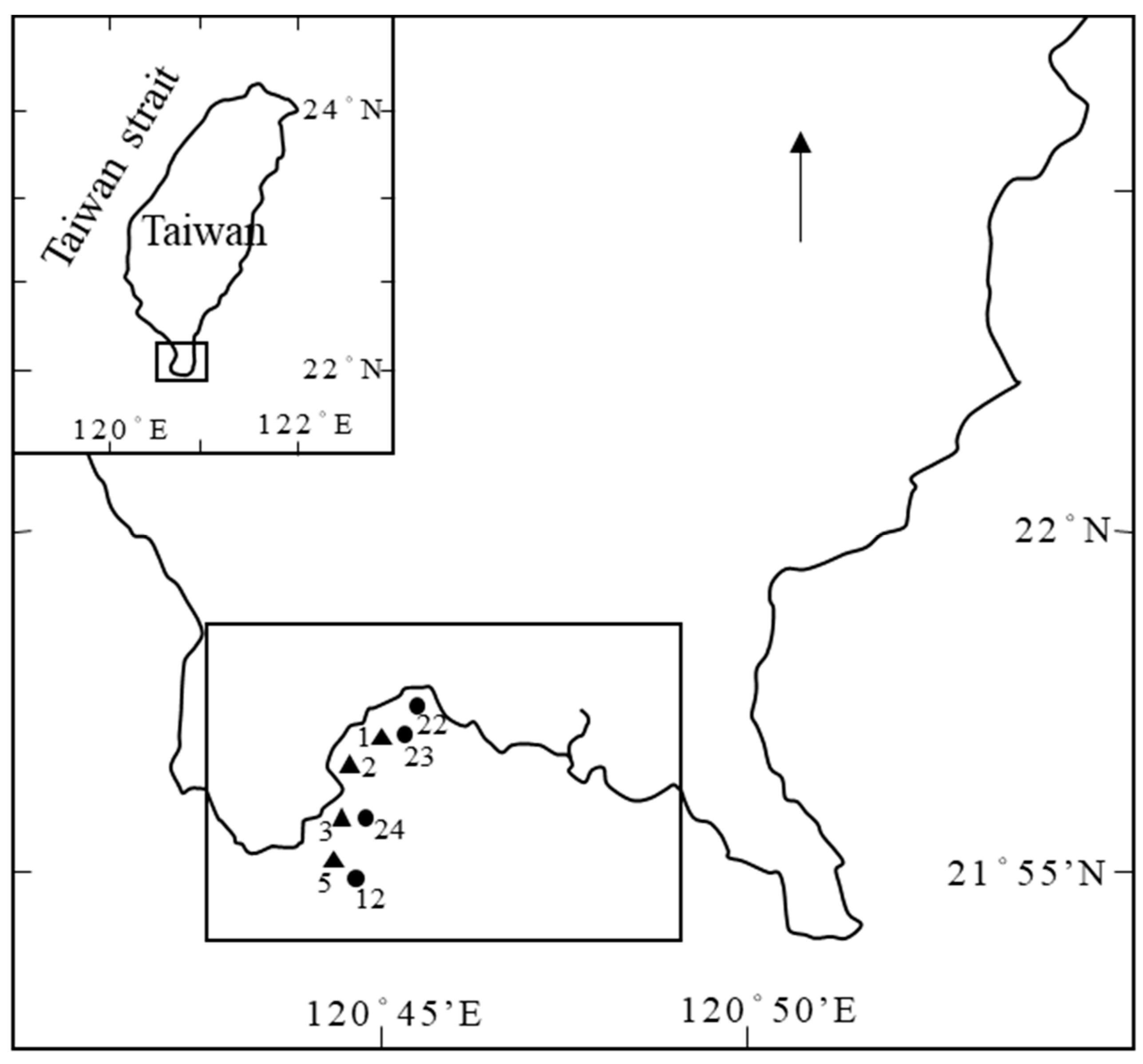
In the field of factor analysis, each variable possesses a distinct meaning, and the extracted factors themselves hold unique significance. Typically, factors are labeled after variables that display high factor loading, and their collective meaning is synthesized to name the factor. In the present study, water quality samples were obtained from the adjacent sea area of Nan Wan Bay, Kenting, Taiwan. Previous research has indicated that the hydrological environment in the nearby waters is intricate, and the occurrence of upwelling in the bay has been established. As a result, the factors were named after Nan Wan Bay's ocean-environmental variations.
Based on the accumulated findings from various studies conducted in the sea area over the years, and the factor analysis outcomes displayed in
Table 6, three component axes were extracted from the component matrix following rotation. These axes are described below.3.3. Factor analysis on biological variables
The first component axis in the present study encompasses nitrate (0.828), silicate (0.811), phosphate (0.693), and nitrite (0.584), which can account for 25.860% of the variation. The factor loading is positive, indicating a positive correlation among the variables. It is noteworthy that in this study, the majority of the water quality measurement parameters were collected from the water surface. The occurrence of sea surges elevates the nutrient salt from the deep ocean to the surface, leading to a concurrent increase in nutrients. Therefore, this component axis was aptly named "Nutrients."
The second component axis in the current study comprises temperature (-0.836), dissolved oxygen (0.737), and salinity (0.639), accounting for 20.347% variation. The results showed a negative factor loading for temperature, while dissolved oxygen and salinity exhibited positive factor loading, indicating a negative correlation between temperature and dissolved oxygen, and temperature and salinity, but a positive correlation between dissolved oxygen and salinity.
Taiwan is located in subtropical, and the surface of seawater is influenced by solar radiation and is typically warmer. Additionally, the evaporation rate exceeds the rainfall rate, leading to an increase in seawater salinity. The waters near Nan Wan Bay are impacted by surges, which transport colder water from deep mid-levels to the surface. As deep mid-level waters lack light and photosynthesis, dissolved oxygen is not saturated, resulting in an overall decrease in dissolved oxygen and temperature when such water surfaces. However, other studies have suggested that Nan Wan Bay is also influenced by internal ocean waves, which cause intense water agglomeration at the seabed and increase dissolved oxygen at the surface. Considering the location of the study in an inland bay and the highest correlation coefficient between temperature drop in the component axis and factor 2 (-0.836), the component axis was named "upwelling current."
3.3. Factor Analysis of Environmental Variables
After factor analysis for environmental variables, the next step is to factor analyze biological variables.3.3.1. First factor analysis
3.3.1. First Factor Analysis
With a KMO value of 0.73, it was considered a "fairly acceptable" fit. Furthermore, the Bartlett's sphericity test was significant at p<0.001, indicating the appropriateness of performing factor analysis on the biological variables of interest. The results of factor extraction revealed two eigenvalues greater than 1, which together explained 54.507% of the total variance.
The second step involves performing a factor rotation using the varimax method of orthogonal rotation. After the rotation, factor 1 (shrimp, number of zooplankton, larvae, crabs) can explain 36.064% of the variance; factor 2 (number of fish, number of fish species, fish eggs) can explain 18.444% of the variation. Based on the findings, it appears that the biological variables related to the "fish eggs" exhibit factor loadings of less than 0.5 in both component axes 1 and 2, indicating a lack of convergent validity. To determine the adequacy of the remaining variables, the communality values of factors 1 and 2 were examined, with a threshold of 0.5 or greater. The communality value for "fish eggs" is only 0.162, the lowest among all the biological variables. Therefore, "fish eggs" is removed for the second round of factor analysis.
3.3.2. Second Factor Analysis
The results of the second factor analysis presented a KMO value of 0.749 indicating a "fair" fit. Moreover, Bartlett's sphericity test was significant (p<0.001), suggesting that the biological variables were appropriate for factor analysis after the removal of the "fish eggs" variable.
After the factor extraction, only two components were reserved for the factor rotation process. The rotation factor 1 (shrimp, number of zooplankton, juvenile larvae, crabs) can explain 42.180% variation; factor 2 (number of fish, number of fish species) can explain 20.377% variation while none of the factor loadings in factors 1 and 2 are greater than 0.5 simultaneously, which suggests that factors 1 and 2 have discriminant validity. Hence, the results from the second factor analysis were preserved for further analysis as shown in
Table 8.
3.3.3. Factor Naming
Based on the results of the previous studies in the sea area and the analysis of the factor extraction in
Table 8, the two factors were named as described below.
The first principal component axis, comprised four biological variables, namely shrimp larvae (0.886), number of zooplankton (0.855), fish larvae (0.773), and juvenile crabs (0.634), which collectively account for 42.180% of the total variation. The factor loading for each variable was positive, implying a positive correlation between them. Zooplankton, in particular, is widely distributed and has a larger number of species, including copepods. Fish larvae and juvenile crabs are also ecologically significant in terms of fishery resources. Previous studies have shown that the intersection of Kuroshio and upwelling currents support diverse flora and fauna[
24,
25]. The number of juvenile shrimp (0.886) and zooplankton (0.855) in the first component axis exhibited a higher correlation coefficient with factor 1, indicating that the sea during the previous sampling period had a higher abundance of zooplankton, especially crustaceans, which are the main food source for fish larvae. Consequently, this component axis was termed “zooplankton cluster”.
The second component axis was composed of two variables, namely the number of fish (0.779) and the number of fish species (0.759), which can explain 42.180% of the variation. The factor loadings of both variables were positive, suggesting a positive correlation between them. The phenomenon of fish migration in groups during foraging season and the formation of fishery in areas with abundant zooplankton can lead to a higher number of fish [
26]. Thus, the name "fish cluster" was given to this component axis.
3.4. Structural Equation
Given the different units of measurements among the variables in the proposed structure, factor analysis was utilized to extract potential factors, namely nutrient, upwelling, primary productivity, zooplankton cluster, and fish cluster, to investigate the interplay between water quality and plankton assemblage, as well as plankton clustering and fish clustering. To test the hypothesis model, this study employed the sampling data assuming a normal distribution. The estimation model assumed that the measured variables of the latent factors were consistent with those presented in
Table 6 and
Table 8. Notably, the sign of coefficients of the latent factor “upwelling current” differed from the factor loading in
Table 6 where the negative values was denoted by the [-] symbol in the model.
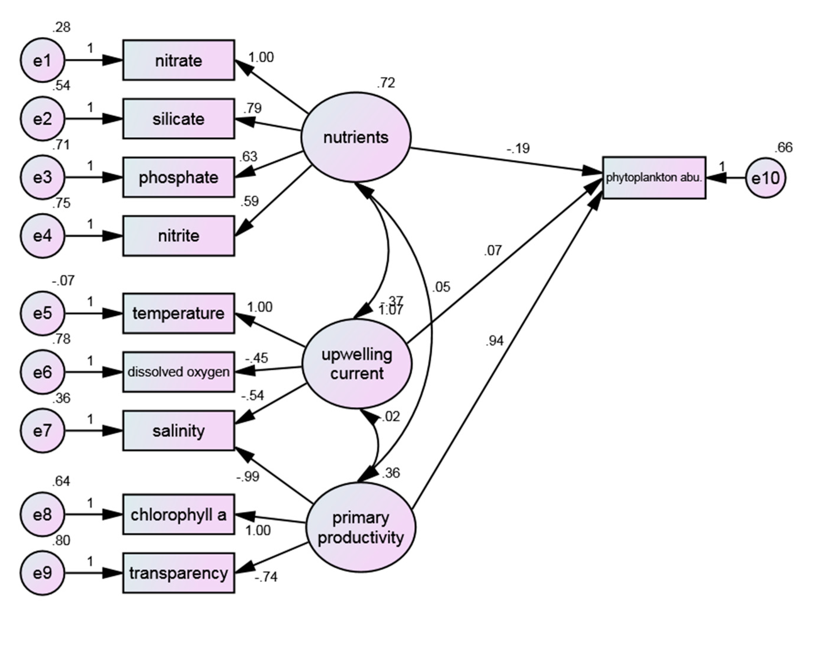
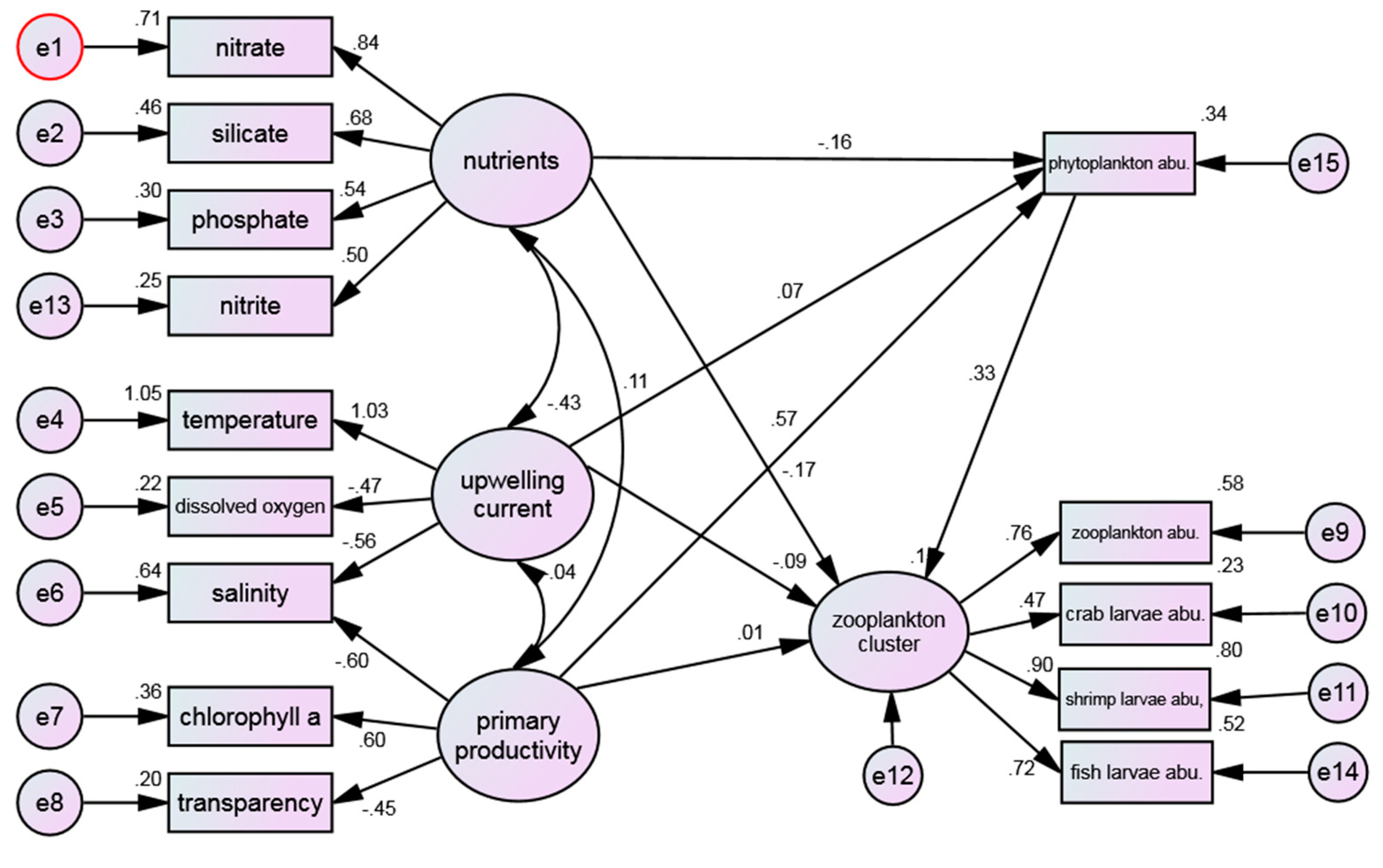
3.4.1. Water Quality Environmental Factors and Phytoplankton Cluster
Figure 3 shows the structure pattern between water quality environments and phytoplankton cluster. The RMSEA (0.113) is in the range of “bad fit”, indicating that the setting of the study model cannot be effectively matched with the sampling data, and the rest of the indicators are not up to the reference criteria. The overall model has not passed the test.
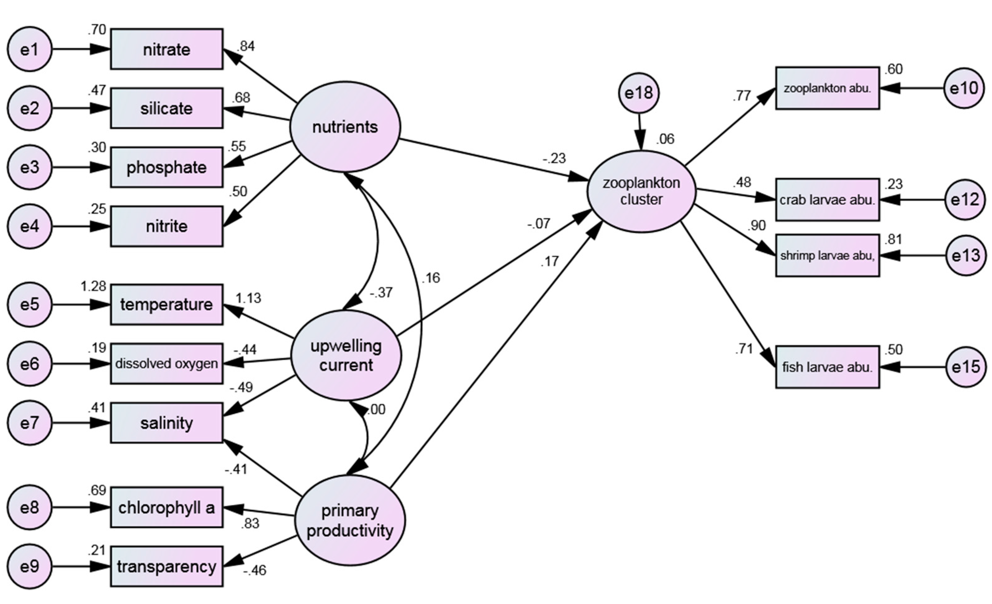
3.4.2. Water Quality Environmental Factors and Zooplankton Cluster
Figure 4 shows the structure pattern between water quality environments and zooplankton cluster. The RMSEA (0.085) value obtained from the model fit analysis (0.085) falls within the range of "moderately fit", albeit falling short of the optimal reference value of less than 0.05. However, the obtained value is still considered acceptable, indicating that the conceptual model proposed is in line with the empirical data obtained. Meanwhile, the non-normed fit index (NNFI) value (0.842) does not meet the reference criteria, which was used to assess the degree of association between the research model and the observed variables and to identify areas for model improvement. Hence, adjustment is needed for covariate relationships.
3.4.3. Water Quality Environmental Factors and Plankton Cluster
Figure 5 shows the structure pattern between water quality environments and both phytoplankton and zooplankton clusters. The index shows that the RMSEA value (0.097) is indicative of a "moderate" fit, although it is close to the threshold of a poor fit. This suggests that the model and the sampling data had only a low degree of probability event and couldn’t effectively explain the results. Furthermore, the NNFI value (0.787) did not meet the reference criteria. The GFI value (0.892) also did not meet the reference criteria. GFI is primarily used to test the proportion between the variance of the explainable observed variables before model adjustment and covariance. However, AGFI (0.831) met the criteria. It was hypothesized that the model must provide more observational data to enhance the degree of interpretation of the observed variables for the potential variables.
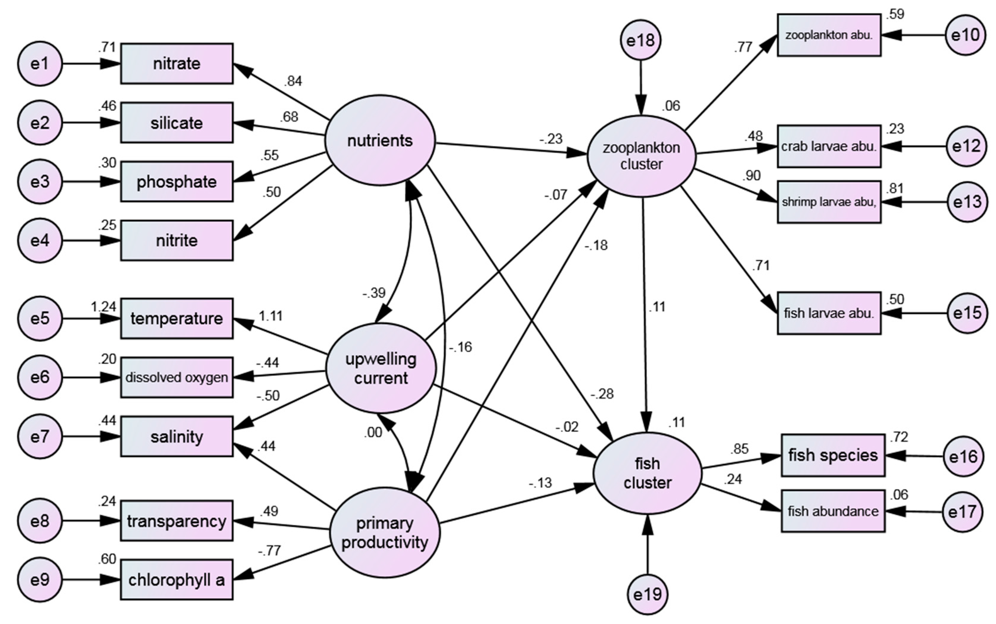
3.4.4. Water Quality Environmental Factors and Marine Life Cluster
The structure that included all three clusters was also considered. However, due to the high correlation between chlorophyll a and the phytoplankton cluster, the model reserves chlorophyll a to represent the primary productivity and dropped phytoplankton cluster.
Figure 6 shows the comprehensive structure pattern between water quality environments and both zooplankton and fish clusters. Of all the indices utilized, only NNFI (0.840) falls short of meeting the reference value and therefore requires further refinement of the model. The remaining indices have successfully passed the test, with RMSEA (0.074) reaching a level of good fit. This suggested that the model has the potential to effectively explicate marine-ecological phenomena to a significant extent.
In the present study, the proposed hypothesis model examining the relationship between environmental factors and marine-life clusters failed to meet the NNFI criteria. This may be due to several factors, including the nature of the sample itself, environmental changes, such as seasonal and weekly-daily fluctuations, and the accuracy and stability of the measuring instrument, which may result in a higher probability of standard errors (non-normal distribution) in the measurement variables. Furthermore, various potential environmental factors, such as sea tide and internal wave phenomena, in the Nan Wan Bay were not included in the statistical analysis. As a result, the proposed model is limited to explaining ecological phenomena only in the sampling waters and may not be applicable to other waters.
3.5. Model Modification
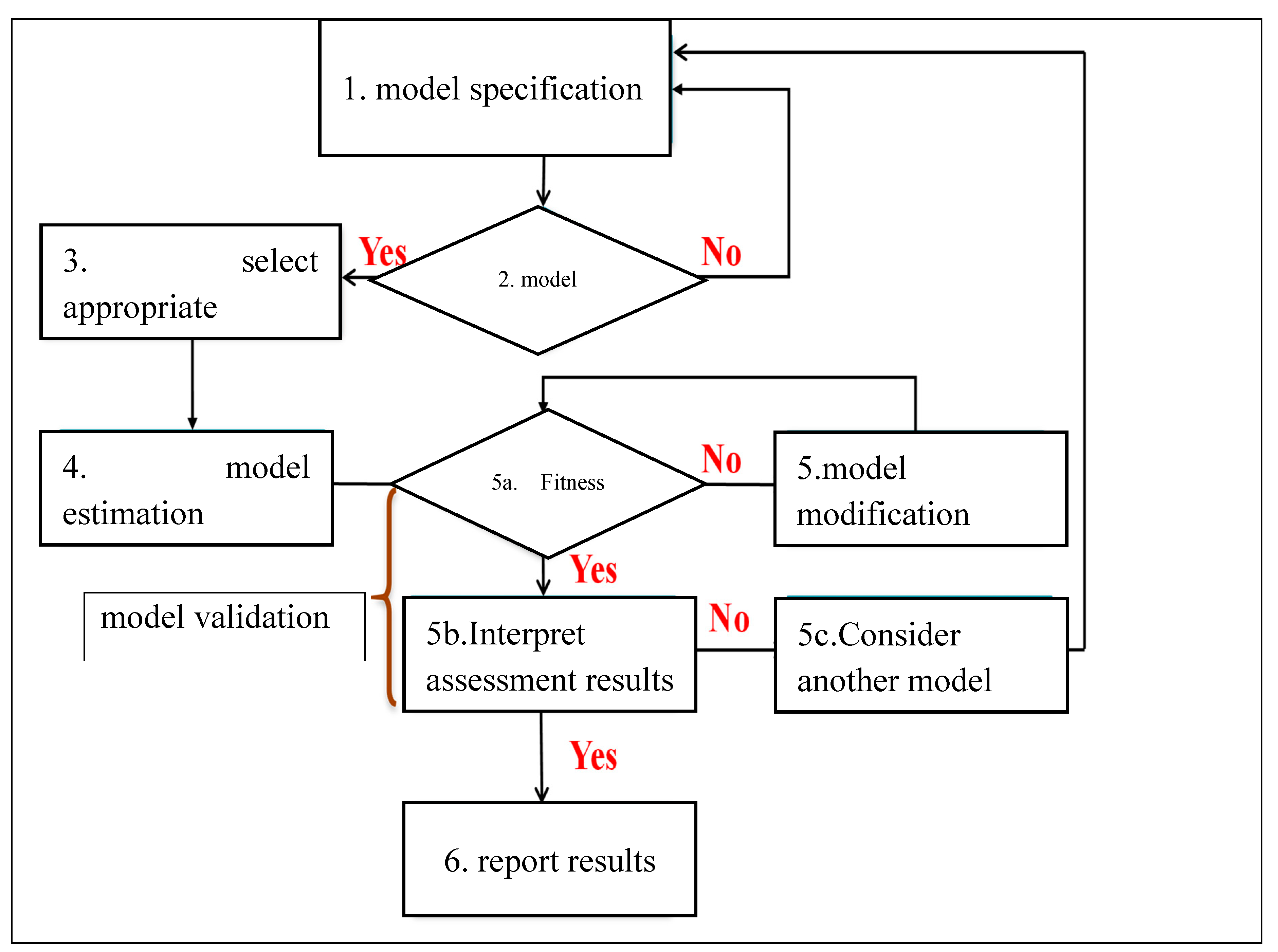
Continuing with the results of the model verification, the next step involves model modification. Due to the covariant relationship between observed variables in the model, parameters in the Modification Index (MI) provided in the Amos Graphics software can be used to modify the model. The main objective of model modification is to improve its simplicity, model fit, explanatory power, and reduce measurement error and structural residuals. However, there is a risk of losing the characteristic of verification and converting the model into an exploratory tool. In the context of the measurement model, one way to modify the model is to allow correlation between measurement variables when supported by theory or literature.
The objective of this study is to explore the correlation between the variables presented in
Figure 5 and
Figure 6. During the model verification phase, the Root Mean Square Error of Approximation (RMSEA) for the models shown in
Figure 4,
Figure 5 and
Figure 6 are all in the moderate fit range (0.08 to 0.10). Notably, the model depicted in
Figure 6 achieved a better fit range (0.05 to 0.08). As the correlation of the variables in the model of
Figure 4 is included in the model of
Figure 5, only the models in
Figure 5 and
Figure 6 were considered for revision.
The model in
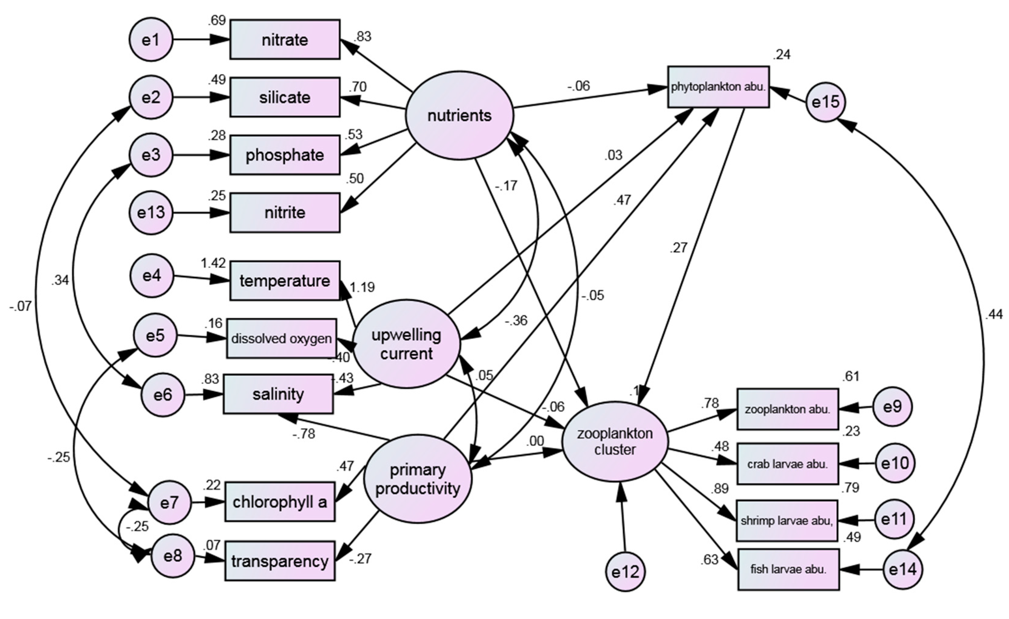
Figure 5 was modified based on the MI value provided in the Amos report by establishing the correlation between residuals of measured variables. Specifically, the correlation between measured variable residuals was increased to reduce the chi-square value, following the principle of modifying one parameter at a time. The revised model is shown in
Figure 7. After the revision, the NNFI (0.939) was in accordance with the reference criteria, and the rest of the indexes also provided validation for the model, especially RMSEA (0.052) reached the range of well fit, indicating that the model and observed data achieved the desired fitting (
Table 9).
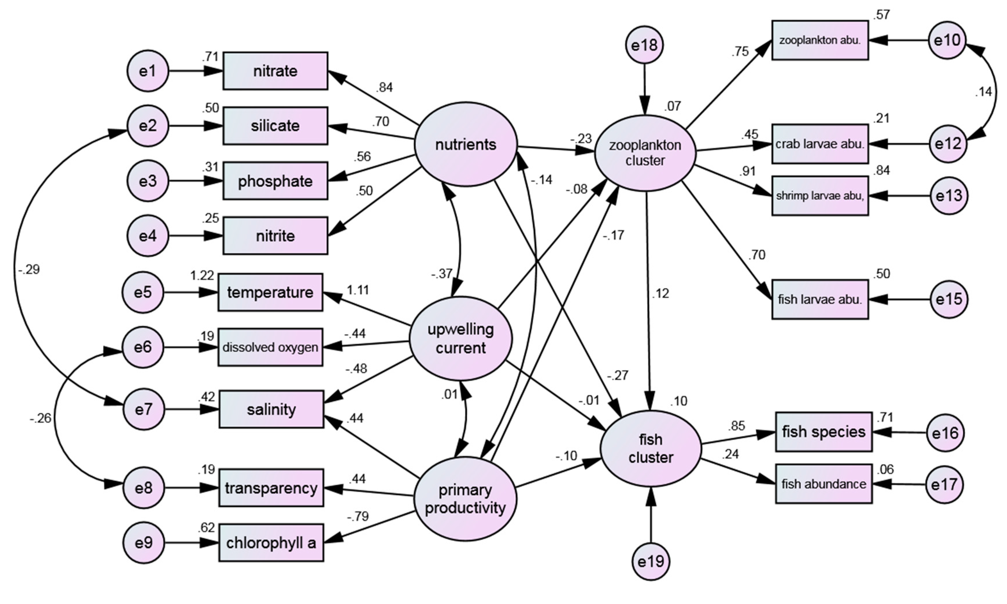
Figure 8 is the revision of
Figure 6, and the results are shown in
Table 10. It can be observed that the Normalized Fit Index (NNFI) attained a value of 0.912, which met the established reference criteria. Furthermore, the other indices also provided validation of the model, with particular emphasis on the Root Mean Square Error of Approximation (RMSEA) which fell within the well-fit range at 0.055. This indicated that the model and the observed data achieved the desired level of fit.
Upon completion of the model revision, subsequent path analysis and the effect between variables were conducted to verify the assumptions made in this study.
3.6. Path Analysis
In addition to evaluating the overall fitness of the model modification and the intrinsic quality of the test, further examination is required to comprehend the linear association between the latent variables. This can be achieved through the observed direct effects and indirect effects to determine the direct and indirect impacts, as well as overall impacts (direct and indirect effects) among the latent variables.
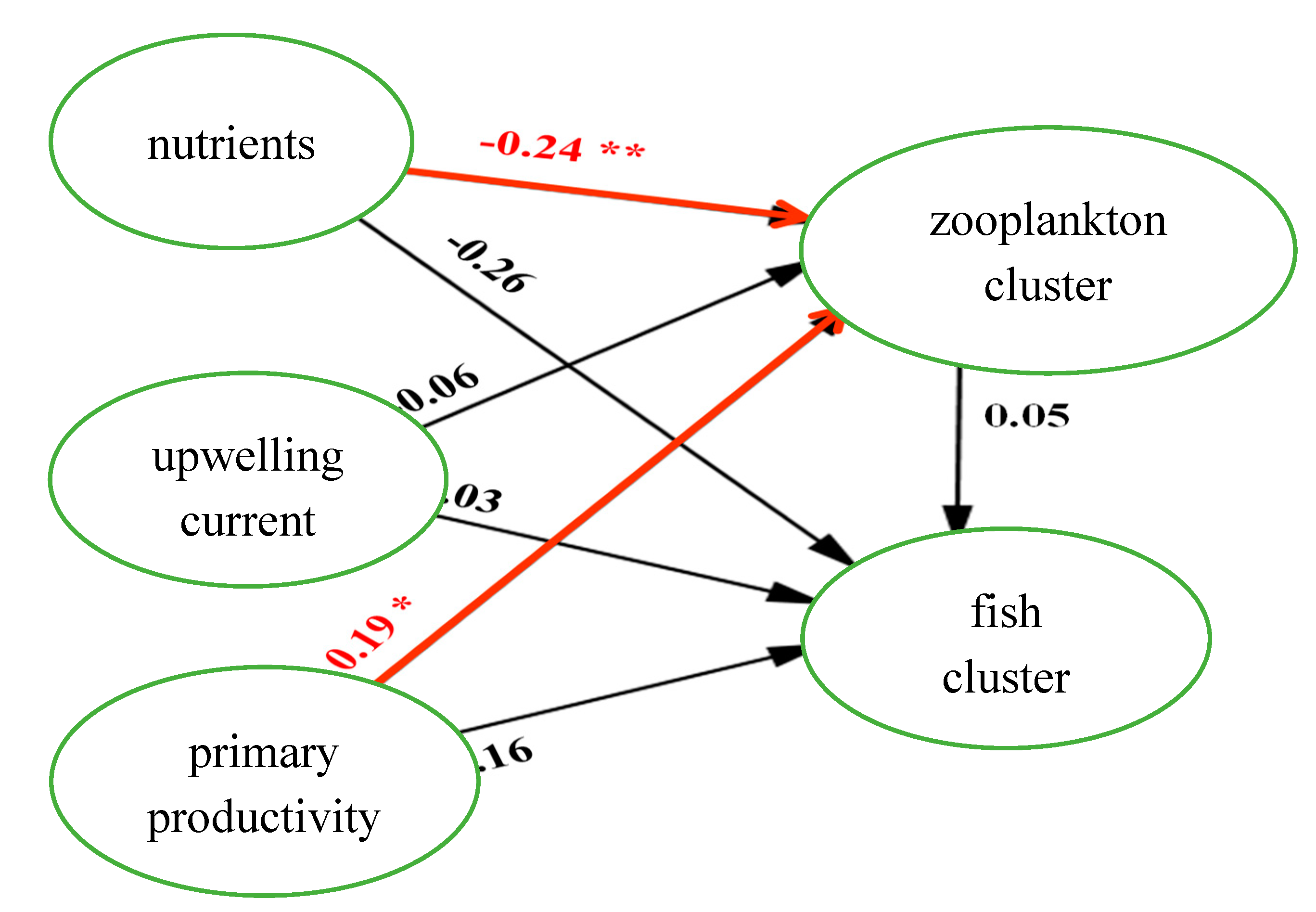
The path relations between the facets were estimated by the structural equation model. The standardized coefficients were used to determine the relationship between the latent variables in the model, as depicted in
Figure 7 and
Figure 8. In
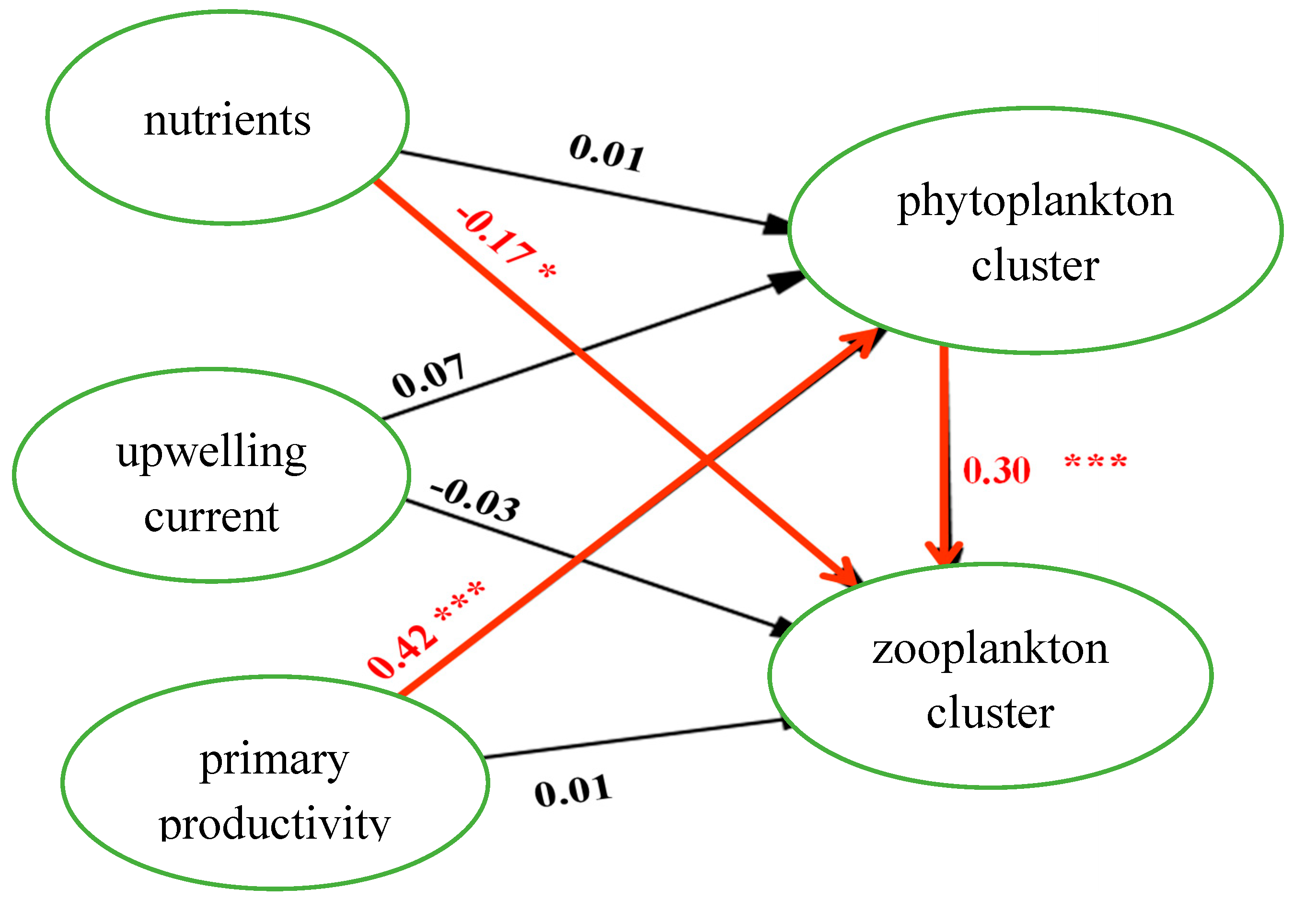
Figure 9, the path effects of "nutrient on zooplankton clustering," "primary productivity on phytoplankton clustering," and "phytoplankton clustering on zooplankton clustering" were found to be statistically significant. Similarly, in
Figure 10, the path effects of "nutrient on zooplankton clustering" and "primary productivity on zooplankton clustering" were also significant, indicating that both models possess considerable predictive capabilities for assessing direct and indirect effects (enhancement or offset) on environmental and biological factors.
The path analysis provides empirical evidence of the direct and indirect effects. The direct effects of nutrients on the zooplankton cluster, primary productivity on the phytoplankton cluster, and phytoplankton cluster on the zooplankton cluster were found to be statistically significant (H2, H5, and H7, respectively). Additionally, the direct effects of nutrients on the zooplankton cluster and primary productivity on the zooplankton cluster were also statistically significant (H8 and H12, respectively). Among the significant direct effects, the effect of primary productivity on the phytoplankton cluster (H5) is the strongest (0.421).
In addition to the direct effects, the study also examined the indirect effects of the predictor variables on the zooplankton cluster. The results in
Table 11 and
Table 12 indicated that, except for the path of primary productivity on the zooplankton cluster, which has a rather higher coefficient of 0.122, the remaining paths have lower coefficients. Therefore, the direct effects were found to be more significant than the indirect effects.
Overall, the study suggests that the marine environment is subject to various factors that may influence the relationships among nutrient salt, primary productivity, phytoplankton cluster, and zooplankton cluster. This may explain why the indirect effects were not significant in this study. It is also possible that there are other intermediary variables or relationships that were not included in the structural statistics, or that the data itself had a high degree of variation.
