1. Introduction
Structural health monitoring (SHM) aims to evaluate large civil and mechanical infrastructures' structural integrity, reliability, and resilience[
1,
2]. The proper implementation of SHM ensures the functioning of these engineering structures by finding structural defects or irregularities before they cause catastrophic structural breakdown [
3]. It involves measuring and evaluating the state properties of the underlying structure and relating these to define the performance parameter. Structural Health Monitoring (SHM) is an emerging field with immense industrial significance, incorporating innovative technology and evolving into a multidisciplinary area of research and development. Despite its growing importance, a recent study has yet to prove enough in many aspects. One primary concern is the reliability quantification of SHM systems, as current assessments primarily rely on visual inspections, which can be subjective and infrequent. On the other hand, existing data processing methods faced challenges from ambient noise, the volume of measurement data, the computation complexity etc. [
4]. These limitations hinder the widespread application of SHM across various industries [
5].
The last decade has seen significant advances in machine learning, particularly in deep learning. Deep learning approaches are very effective in various tasks, yielding cutting-edge outcomes across multiple engineering disciplines [
6]. Recent advancement in artificial intelligence has also provided an opportunity to address these SHM challenges and elevate the capability and applicability of the SHM sector [
7,
8].
Recently, Rai and Mitra [
9] proposed a 1D convolutional neural network (CNN) to detect damage in Aluminum metallic structures. The proposed method can process raw signals and identify the different types of structural damage. Similarly, Wang et al. [
10] presented a structural damage identification method based on integrating Hilbert-Huang transformation and CNN. Similarly, the author used a DNN with an autoencoder to compress the input data and a second neural network architecture to translate the compressed input into the damage characteristic. For guided wave (GW)-based fatigue crack diagnosis (FCD) on aluminium-alloy attachment lugs, Xu et al. [
11] developed a CNN model. The trained multiclass CNN model predicted the crack length with an accuracy of 86.84%.
Similarly, Li
et. al. [
12] employed a deep CNN network on a bridge. The author determined the deflection signal from the fibre-optic gyroscope sensor. The author exploited a data augmentation scheme to enhance the size of the datasets. The trained model generates an efficiency of 97% and outperforms many traditional Machine Learning algorithms. Many authors integrate multiple deep-learning networks. For example, [
13] combined 1D CNN and LSTM for acceleration data obtained from a three-story frame. The combined architecture decreases the computational cost, but the network is noise-sensitive.
Most of the damage detection strategies based on deep learning methods are mainly supervised and require data preprocessing and filtering methods to extract its key features. Moreover, most of the traditional deep learning methods require large amounts of training datasets, which is an expensive and time-consuming effort, requires experts' knowledge, and hence generates a bottleneck in the automation system.
In this paper, we trained a biLSTM-based autoencoder with maximal overlap discrete wavelet transform (MODWT) layer to accurately predict the signal anomaly and detect the presence of structural damage and, based on this, help to determine the damage location. The rest of the paper is organized as, in section 2, a brief description of the autoencoder, LSTM and MODWT layer is presented, while in the next section, the proposed methodology along with the experimental setup is explained. In the 4th section, anomaly detection and damage localization based on the proposed methodology is performed, while the conclusion is drawn in the last section.
2. Background
2.1. Autoencoder
Autoencoder, a particular type of deep learning network, is trained to replicate the input data. Anomaly detection, text generation, picture generation, image denoising, and digital communications are some areas where autoencoders outperform conventional engineering approaches in terms of accuracy and performance [
14]. Autoencoder is an unsupervised learning traditionally consisting of two parts: encoder and decoder. The encoder compresses the data into a latent space vector, while the decoder tends to convert the latent space vector into the original input.
If the input to an autoencoder is a vector,
then it will convert into another vector
as
Where, h is a transfer function f the encoder, w is a weight matrix, and b is a bias vector. Then the decoder converts an estimate of the original input vector, x, from the encoded representation, z, as follows:
Where the quotation marks represent the other layer. The autoencoder learns to recognize and replicate the "standard" or "healthy" condition of the structural signals. When new data is introduced, the autoencoder tries to reconstruct it based on its understanding of the normal state. If the new data reflects an undamaged state, the autoencoder should accurately recreate it, resulting in a low reconstruction error. If the signal is damaged, containing ambiguous terns, then the autoencoder's attempts to rebuild the data using what it has learned from the undamaged pattern will result in a more significant reconstruction error [
15].
2.2. RNN and BiLSTM
RNNs are a neural networks often employed for sequential data processing jobs. They are intended to deal with input data with temporal dependencies and where the sequence of the data points is essential. RNNs are excellent at applications, including speech recognition, natural language processing, and time series analysis [
16]. The fundamental principle underlying RNNs is that they include feedback links that allow information to persist over time. This feedback mechanism allows the network to maintain memory and capture long-term dependencies in the input [
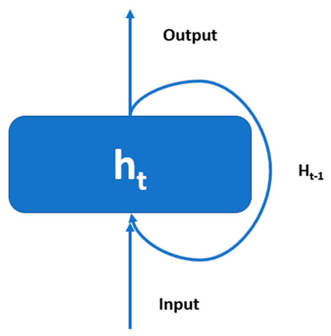
17]. Unlike feed-forward networks such as convolutional neural networks (CNNs), features a recurrent connection. Where the last hidden state is an input to the next state,
Figure 1 presents a typical RNN network.
LSTM layers are RNNs meant to learn and interpret long-term relationships in time-ordered data or sequences. Traditional RNNs frequently struggle to capture these long-term dependencies due to issues with "vanishing" or "exploding" gradients during training. The expressions "vanishing" and "exploding" gradients apply to circumstances in which the gradients become unexpectedly tiny or excessively big. These problems can impede the network's capacity to develop and sustain interactions over long periods. LSTM helps to address these challenges, improving its ability to grasp and recall information across extended periods. It handles gradient issues by incorporating additional gates that govern the flow of information within the hidden cell, determining what information is preserved for output and the next hidden state. With better control over information flow, LSTMs can more successfully learn and imitate long-term connections in data. LSTM are more efficient than conventional neural networks such as ANN and CNN, which are less appropriate for collecting temporal correlations among sensor data [
18].
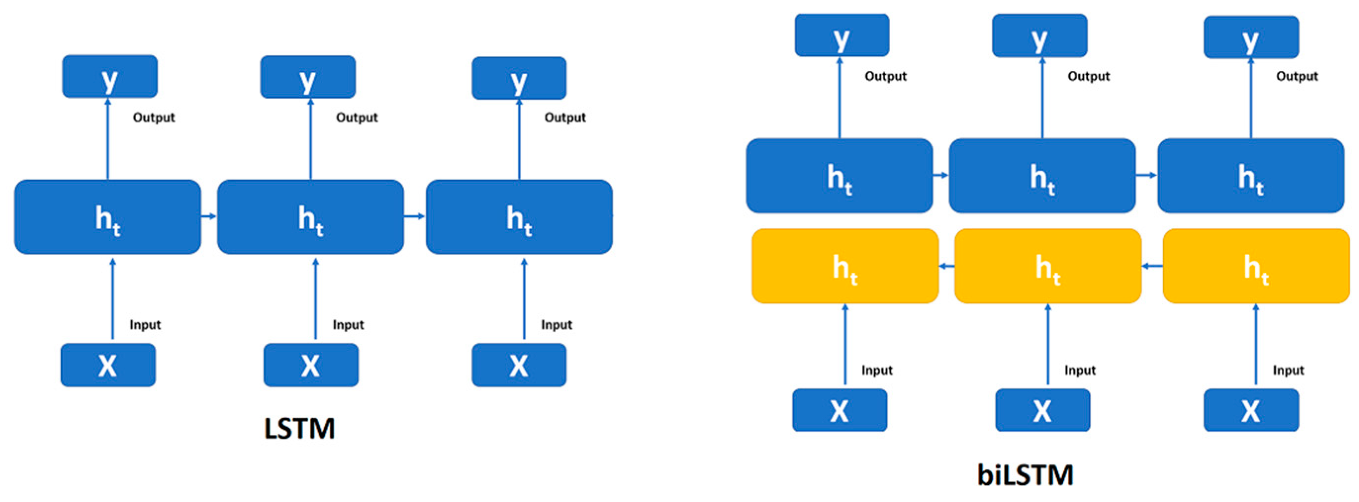
On the other hand, the basic idea behind Bi-LSTMs is to have two independent LSTM layers, one processing the sequence ahead and the other processing it backwards. Each LSTM layer has its hidden state, and at each time step, the outputs of both layers are combined [
19].
Figure 2 represents the general architecture of uniLSTM and biLSTM
2.3. Maximal Overlap Discrete Wavelet Transform:
MODWT uses low- and high-pass filters to split the frequency spectrum of the input signal into scaling and wavelet coefficients. The traditional way of constructing the Maximal Overlap Discrete Wavelet Transform (MODWT) employs circular convolution directly in the time domain. However, the technique presented here performs the circular convolution within the Fourier domain, potentially improving processing efficiency and treating periodic signals [
20].
To elaborate, the wavelet and scaling filter coefficients at a particular level, 'j', are computed by first performing the signal's discrete Fourier transform (DFT) and the wavelet or scaling filter's DFT at the 'jth' level. The DFT is a mathematical approach commonly used for frequency analysis of time-domain signals to transform a function of time into frequency. The product of these DFTs is then computed, which essentially captures the multiplication of their spectral components. This procedure relates to the time domain convolution of the original signals. Finally, the inverse DFT is done on this product which converts the information back into the time domain, producing the wavelet and scaling filter coefficients for the 'jth' level [
21].
This method efficiently computes the circular convolution in the Fourier domain before bringing it back into the time domain. The benefit of this approach is its computing efficiency and precision, which is especially useful for big data sets and when the signal or system of interest is intrinsically periodic or well-represented in the frequency domain.
The jth-level wavelet filter is defined by
The
jth level scaling filter is,
3. Methodology:
3.1. Experimental datasets:
In the paper, we utilized the datasets provided by the Open Guided Waves (OGW) platform [
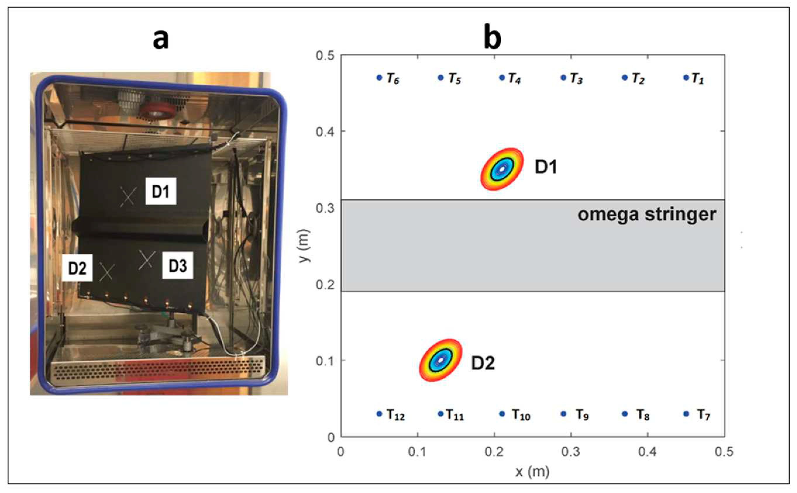
22]. Two carbon fibre plates having dimensions of 550 mm × 550 mm and a thickness of 2 mm are used. The thickness of each layer within the plates is 0.125 mm. Hexply® M21/34%/UD134/T700/300, a particular kind of carbon fibre prepreg material, is used for the plates. A quasi-isotropic (QI) layup pattern is used to organize the layers within the plates, which means the layers are angled differently to offer balanced strength in various directions. The omega stringer, a separate component, is also composed of Hexply® M21/34%/UD194/T700/IMA-12K carbon fibre prepreg material. The stringer features a [45/0/90/45/90/45]S quasi-isotropic layup pattern. The nominal thickness of the stringer is 1.5 mm, and each layer within the stringer has a thickness of 0.125 mm. The complete experiment setup is given in
Figure 3a.
The plate has 12 piezoceramic transducers, and each experiment collects a total of 66 separate signals from the decentralized and dispersed array of transducers' actuator-sensor pairs in a round-robin method,
Figure 3b. The position of these transducers is given in the
Table 1
For anomaly detection, we consider 60kHz Lamb wave excitation frequency. A Hann-windowed five-cycle excitation pulse was generated. For the measurement, Author [
22] considered seven different phases. For phase 1, five measurements were recorded on the pristine structure. In phase two, reference defects were attached to the plate at position 𝐷1. An electromagnet with a metal block pressed the reference damage to the structure for maximum reliability. The electromagnet was then removed, leaving only the reference damage in contact with the structure. This process was repeated five times for each of the 13 damage sizes and positions. In the next phase, the author recorded another five baseline measurements after removing the reference damage. The author followed the same procedures for other damage positions in the next phases. Overall, 20 baseline and 520 damage measurements were recorded. Not that, origionally author used three damage conditions present at different locations; however, in this study, we only considered two damage locations on the plate.
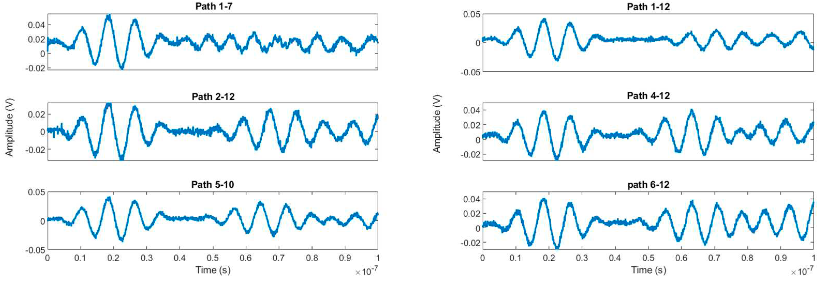
The stringer significantly impacts guided wave propagation, resulting in considerable signal changes. Here the real challenge is used to raw signals and extract useful information related to the state of the structure. To simplify the analysis, we focus only on the signals that traverse the plate and are received by sensors on the opposite side. As a result, out of the total 66 signals, we narrowed our attention to 36 signal paths. Moreover, We considered only 2048 sampling points as we were interested in the first arriving waves and reflections from the damage and stringer. There are 720 datasets of which 90% were used for the training purpose while 10% were for validation. Some of the waveforms are given in
Figure 4
3.2. Model Training:
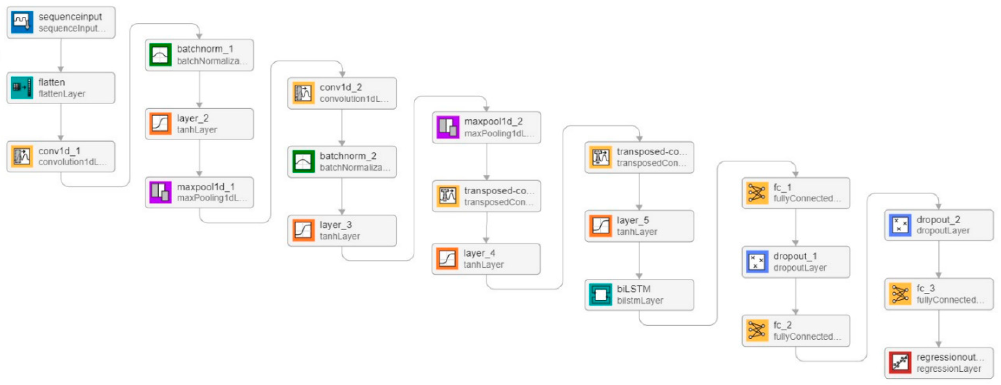
In this study, we exploited three different autoencoders. The first is 1D CNN, in which the convolutional layer performs the function of a feature extractor. It employs appropriate filters or kernels to capture spatial and temporal interdependence in time-varying signals. To train the convolutional autoencoder, we built a hybrid model in which convolutional layers and BiLSTM were simultaneously used. The 1-D convolutional layer first filters the signal and removes the majority of the high-frequency noise. After that, the BiLSTM layer refines the signal features further. There is a total of 21 layers used with an overall 21000 learnable. The
Figure 5 presents the architecture for CNN network
In the subsequent phase, a pure LSTM autoencoder model was developed. This model consisted of multiple bidirectional LSTM layers alternated with ReLU activation layers. These were later followed by a fully connected layer and a regression layer. There are nine layers in the model, with 29,300 learnable parameters. In the third phase, we added the MODWT layer with a multiresolution analysis algorithm in biLSTM architecture. This study used "Coiflets" orthogonal wavelets with five transform levels. The complete architecture is given in
Figure 6 and all parameters are presented in
Table 2.
Adam optimizer was used for training, which is suitable for nonstationary and nonlinear data like Lamb wave signals, with a learning rate of 0.001. The minibatch size was 500, with a maximum epoch was between 200 and 600, depending on the computational complexity. All the training was done using MATLAB® deep learning toolbox while all network architecture was designed and analyzed on the Deep network designer app provided by Mathwork®. Since 90% of baseline datasets are used for the model training, and 10% are used for validation purposes, the table represents the training and validation accuracy.
As observed from the table, when comparing with 1D CNN, it is evident that biLSTM performs better for the given datasets. However, adding the MODWT layer further enhanced the prediction accuracy of biLSTM and resulted in slightly lower RMSE values. The model with biLSTM and MODWT Layer can capture the signals' peak position, magnitude, and shape well.
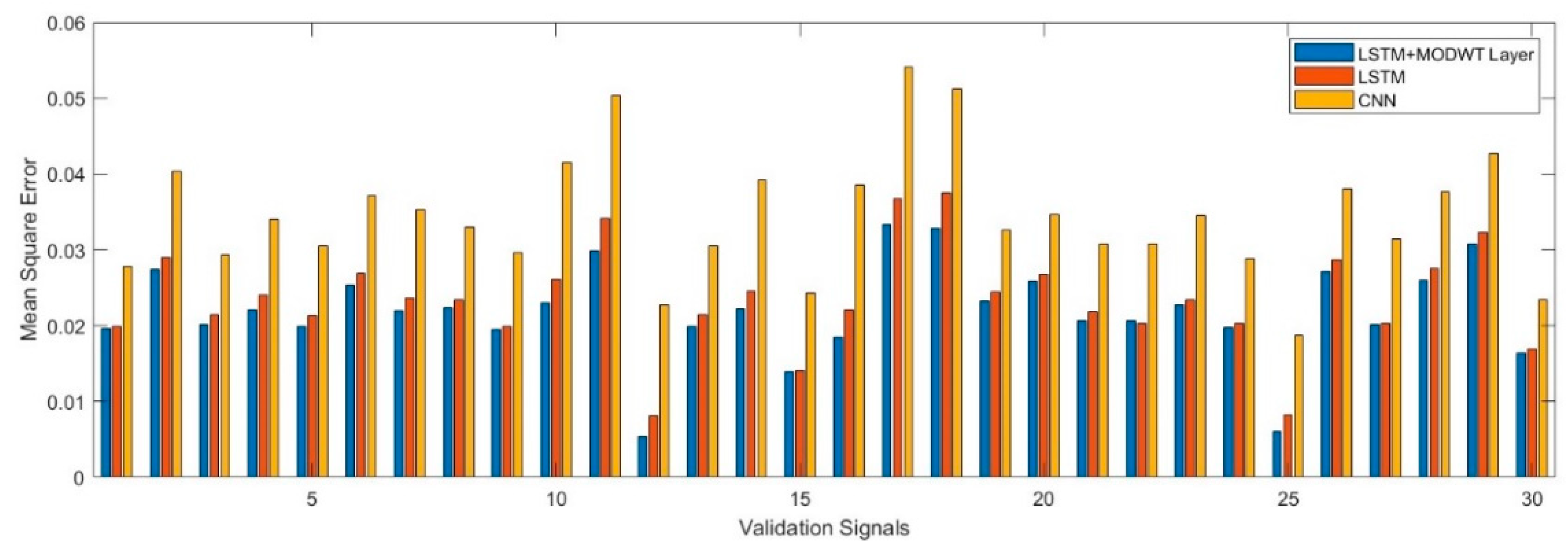
Figure 7 shows the validation mean square error for all three architectures. Since there are 7 validations signals, we only present the first 30 signals here. It can be observed that the biLSTM with MODWT layer outperforms the other deep learning scheme and generate signals with better quality. Furthermore, the
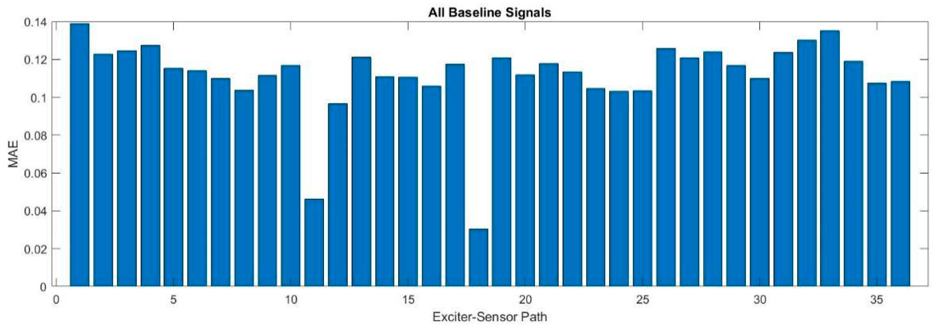
Figure 8 shows the MAE for all exciter-sensor paths for all given datasets, determined by the proposed method.
4. Methodology:
4.1. Anomaly Detection:
An autoencoder model-based anomaly detection system is usually trained solely on data corresponding to the pristine signal condition. As a result, the model is equipped to precisely reconstruct input that closely reflects inherent signal trends. Consequently, we can determine whether an input is an anomaly by examining its reconstruction error. The system classifies the input as an anomaly if the error surpasses a well-defined threshold. However, if the reconstruction error stays below this cutoff, the input is regarded as normal and consistent with typical normal signal patterns. The strength of this approach depends on the ability to identify unique signals variation. Since the model is trained only on pristine data, any significant deviation in the input, even one that doesn't align with known signal patterns, would lead to a higher reconstruction error. This means that the autoencoder can detect or flag anomalies as long as patterns deviate from the learned normal patterns.
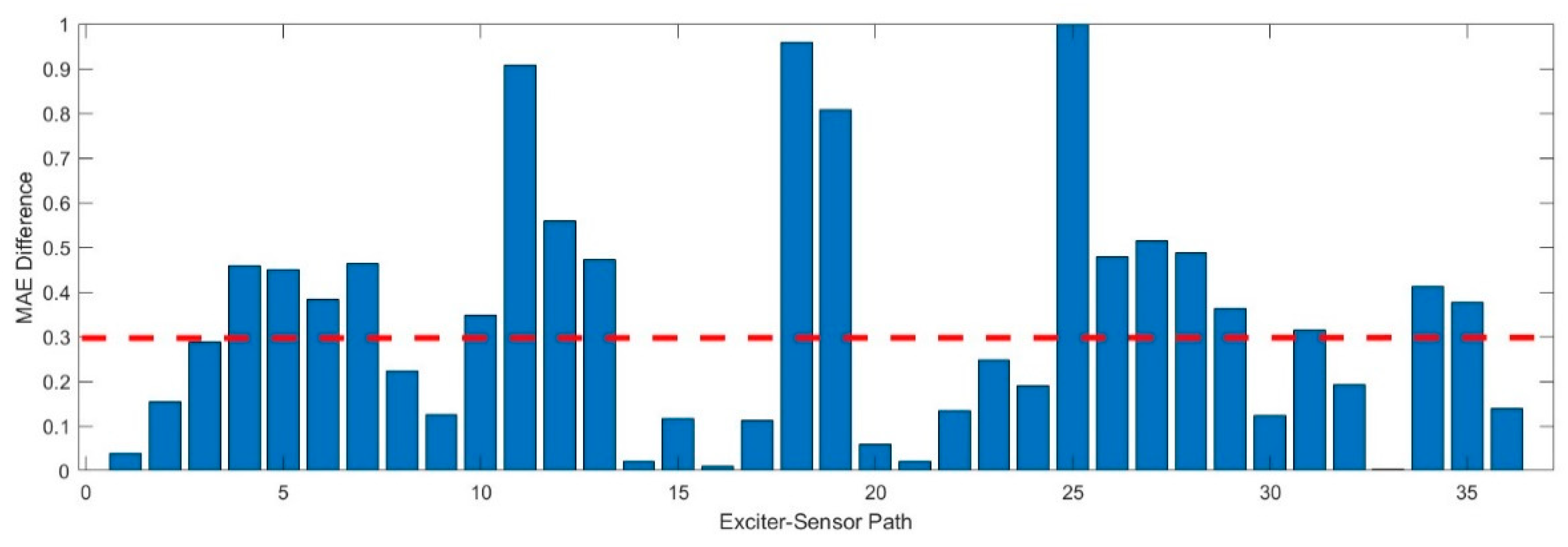
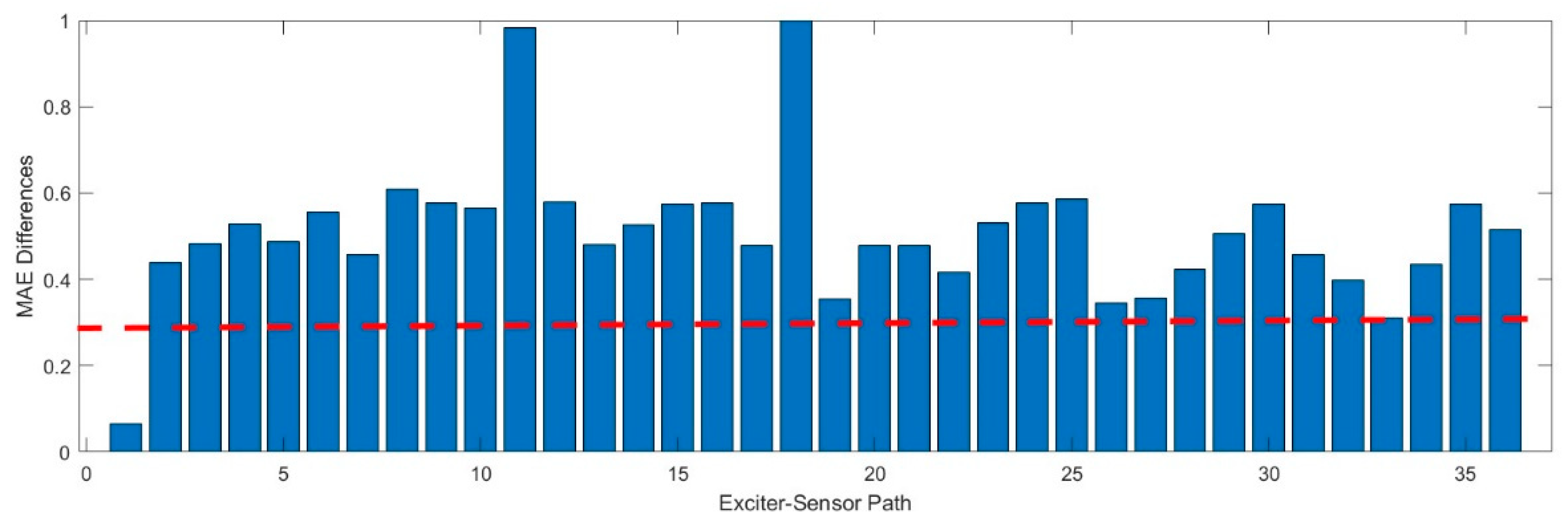
This study considers two damages placed at different locations, as shown in the table. We use damage datasets for D1 and calculate the MAE. The MAE difference in normalized was determined by comparing it with the baseline signal, as shown in
Figure 9. We set the threshold value equal to be equal to 0.3. This value was determined empirically by analyzing the baseline signals and validation data.
It can be observed that different bars surpassed the threshold value. Each bars in the
Figure 9 represents a different pathway from the exciter sensor. Studying these bars, we can better understand which paths may pass through the damaged. Similar to identifying anomalous signals, this visualization aids in detecting irregularities or deviations that might signify damage in specific paths. Similarly,
Figure 10 shows error values for D2 which shows significant deviations from the learner learned pattern. It is also observed that peaks in both the Figure generated when the exciter-sensor path directly passes or is close to the damage. The
Table 3 shows the average MAE values for D1 and D2.
Table 3.
Average MAE for both damage.
Table 3.
Average MAE for both damage.
| Damage ID |
MAE difference |
| D1 |
0.37 |
| D2 |
0.48 |
4.2. Damage Localization:
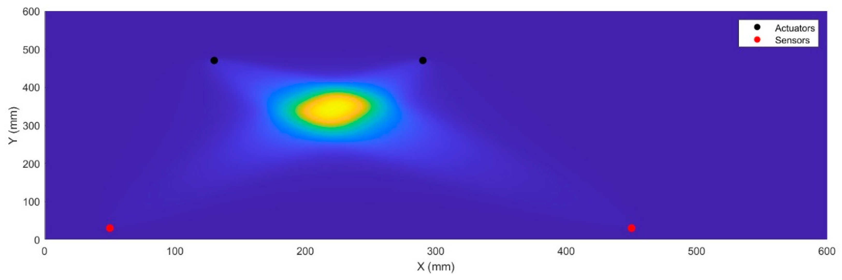
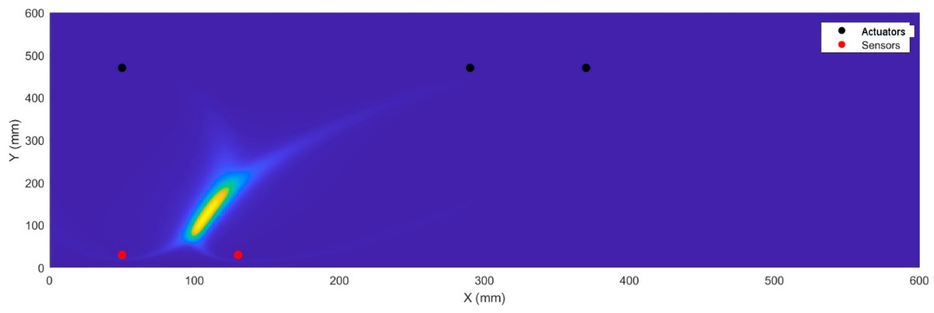
In this section, we apply a reconstruction algorithm to localize the damage on the plate. For this purpose, we only considered those exciter-sensor paths with maximum peak values; hence, these peak values were used as weights for the pixels. We first subtracted the damage signal from the pristine signal and then determined the signal envelope. Here we exploited time-frequency transformation for this purpose. In this section, we implement a reconstruction algorithm to pinpoint the location of damage on the plate. To facilitate this, we limit our focus to the exciter-sensor paths that display the highest peak values. The first step in this process involves subtracting the pristine, undamaged signal from the damaged signal. Subsequently, we ascertain the signal envelope. We utilize a time-frequency transformation to leverage its capabilities to identify and analyze signal components effectively. In addition, we utilized the normal distribution to reduce the width of the generated signal envelope. This technique involves using the maximum peak value of the signal as the mean (average) of the normal distribution. The normal distribution, also known as the Gaussian distribution, is a symmetric probability distribution about the mean. By centering this around the maximum peak value, we effectively narrow the envelope's width, focusing more precisely on the region of interest within the signal. This technique provides a more focused and accurate understanding of where potential anomalies, such as damage, might occur within the signal.
The
Figure 11 and 12 show the location of the damage D1 and D2 respectively. As we can observe, the position of D1 was determined by utilizing only two exciter-sensor paths. As proposed autoencoder scheme accurately determined which exciter-sensor paths are optimal for localized damage. However, the result can be precise by adding more paths.
5. Conclusions
This study used an autoencoder that integrated a Bi-directional Long Short-Term Memory (BiLSTM) layer with a Maximal Overlap Discrete Wavelet Transform (MODWT) layer. This configuration aimed to identify anomalies in Lamb wave signals as they propagated through a composite structure. Our deep learning approach was trained on 720 raw baseline signals, encompassing 36 distinct exciter-sensor paths. This proposed method was validated using unseen datasets comprising 72 randomly selected signals. One of the primary strengths of our approach is its ability to work directly with raw oscilloscope signals, thus eliminating the need for extensive data preparation. To ascertain the effectiveness of our method, we compared the validation accuracy with that of a pure LSTM-based deep model and a 1D Convolutional Neural Network (CNN) model. The results demonstrated that our proposed method performed admirably. To detect anomalies, we introduced damaged signals to the trained encoder model and established threshold values derived from the error generated by the model on the baseline signals. We observed that data sets involving multiple exciter-damage paths exceeded these threshold values, indicating structural damage.
Interestingly, paths that passed close to or directly across the damage produced higher error values. This observation proved instrumental in accurately identifying the precise location of the damage within the structure. This approach has the potential to greatly enhance our ability to detect and locate structural damage in composite structures, thereby increasing safety and efficiency.
Author Contributions
Syed Haider Mehdi Rizvi performed the major research work and writing. Muntazir Abbas provide assistance and supervision on this project. Syed Muhammad Tayyab provide technical support and assistance to complete this research project.
Funding
Major APC was funded by the National University of Science & Technology (NUST)
Conflicts of Interest
The funders had no role in the design of the study; in the collection, analyses, or interpretation of data; in the writing of the manuscript; or in the decision to publish the results.
References
- Cho, S.; Yun, C.-B.; Lynch, J.P.; Zimmerman, A.T.; Spencer Jr, B.F.; Nagayama, T. Smart Wireless Sensor Technology for Structural Health Monitoring of Civil Structures. Steel Structures 2008, 8, 267–275. [Google Scholar]
- Giurgiutiu, V. Structural Health Monitoring with Piezoelectric Wafer Active Sensors: With Piezoelectric Wafer Active Sensors; Elsevier, 2007; ISBN 0080556795.
- Giurgiutiu, V. Lamb Wave Generation with Piezoelectric Wafer Active Sensors for Structural Health Monitoring. In Proceedings of the Smart Structures and Materials 2003: Smart Structures and Integrated Systems; International Society for Optics and Photonics; 2003; Vol. 5056, pp. 111–123. [Google Scholar]
- Ye, X.W.; Jin, T.; Yun, C.B. A Review on Deep Learning-Based Structural Health Monitoring of Civil Infrastructures. Smart Struct Syst 2019, 24, 567–585. [Google Scholar]
- Alazzawi, O.; Wang, D. Damage Identification Using the PZT Impedance Signals and Residual Learning Algorithm. J Civ Struct Health Monit 2021, 11, 1225–1238. [Google Scholar] [CrossRef]
- Ye, X.W.; Jin, T.; Yun, C.B. A Review on Deep Learning-Based Structural Health Monitoring of Civil Infrastructures. Smart Struct Syst 2019, 24, 567–585. [Google Scholar]
- Zhang, Z.; Pan, H.; Wang, X.; Lin, Z. Machine Learning-Enriched Lamb Wave Approaches for Automated Damage Detection. Sensors 2020, 20, 1790. [Google Scholar] [CrossRef]
- Zhang, Z.; Sun, C. Structural Damage Identification via Physics-Guided Machine Learning: A Methodology Integrating Pattern Recognition with Finite Element Model Updating. Struct Health Monit 2021, 20, 1675–1688. [Google Scholar] [CrossRef]
- Rai, A.; Mitra, M. Lamb Wave Based Damage Detection in Metallic Plates Using Multi-Headed 1-Dimensional Convolutional Neural Network. Smart Mater Struct 2021, 30, 35010. [Google Scholar] [CrossRef]
- Wang, X.; Zhang, X.; Shahzad, M.M. A Novel Structural Damage Identification Scheme Based on Deep Learning Framework. Structures 2021, 29. [Google Scholar] [CrossRef]
- Xu, L.; Yuan, S.; Chen, J.; Ren, Y. Guided Wave-Convolutional Neural Network Based Fatigue Crack Diagnosis of Aircraft Structures. Sensors 2019, 19, 3567. [Google Scholar] [CrossRef] [PubMed]
- Li, S.; Zuo, X.; Li, Z.; Wang, H. Applying Deep Learning to Continuous Bridge Deflection Detected by Fiber Optic Gyroscope for Damage Detection. Sensors 2020, 20, 911. [Google Scholar] [CrossRef] [PubMed]
- Hung, D.V.; Hung, H.M.; Anh, P.H.; Thang, N.T. Structural Damage Detection Using Hybrid Deep Learning Algorithm. Journal of Science and Technology in Civil Engineering (STCE) - NUCE 2020, 14, 53–64. [Google Scholar] [CrossRef]
- Reconstruct Inputs to Detect Anomalies, Remove Noise, and Generate Images and Text. Available online: https://www.mathworks.com/discovery/autoencoder.html (accessed on 11 June 2023).
- Torabi, H.; Mirtaheri, S.L.; Greco, S. Practical Autoencoder Based Anomaly Detection by Using Vector Reconstruction Error. Cybersecurity 2023, 6, 1. [Google Scholar] [CrossRef]
- Recurrent Neural Network (RNN) . Available online: https://www.mathworks.com/discovery/rnn.html (accessed on 11 June 2023).
- Said Elsayed, M.; Le-Khac, N.-A.; Dev, S.; Jurcut, A.D. Network Anomaly Detection Using LSTM Based Autoencoder. In Proceedings of the Proceedings of the 16th ACM Symposium on QoS and Security for Wireless and Mobile Networks; 2020; pp. 37–45. [Google Scholar]
- Lu, Y.; Tang, L.; Chen, C.; Zhou, L.; Liu, Z.; Liu, Y.; Jiang, Z.; Yang, B. Reconstruction of Structural Long-Term Acceleration Response Based on BiLSTM Networks. Eng Struct 2023, 285, 116000. [Google Scholar] [CrossRef]
- Li, S.; Li, W.; Cook, C.; Zhu, C.; Gao, Y. Independently Recurrent Neural Network (Indrnn): Building a Longer and Deeper Rnn. In Proceedings of the Proceedings of the IEEE conference on computer vision and pattern recognition; 2018; pp. 5457–5466. [Google Scholar]
- Maximal Overlap Discrete Wavelet Transform . Available online: https://www.mathworks.com/help/wavelet/ref/modwt.html (accessed on 11 June 2023).
- Xiao, F.; Lu, T.; Wu, M.; Ai, Q. Maximal Overlap Discrete Wavelet Transform and Deep Learning for Robust Denoising and Detection of Power Quality Disturbance. IET Generation, Transmission & Distribution 2020, 14, 140–147. [Google Scholar]
- Moll, J.; Kexel, C.; Kathol, J.; Fritzen, C.-P.; Moix-Bonet, M.; Willberg, C.; Rennoch, M.; Koerdt, M.; Herrmann, A. Guided Waves for Damage Detection in Complex Composite Structures: The Influence of Omega Stringer and Different Reference Damage Size. Applied Sciences 2020, 10, 3068. [Google Scholar] [CrossRef]
|
Disclaimer/Publisher’s Note: The statements, opinions and data contained in all publications are solely those of the individual author(s) and contributor(s) and not of MDPI and/or the editor(s). MDPI and/or the editor(s) disclaim responsibility for any injury to people or property resulting from any ideas, methods, instructions or products referred to in the content. |
© 2023 by the authors. Licensee MDPI, Basel, Switzerland. This article is an open access article distributed under the terms and conditions of the Creative Commons Attribution (CC BY) license (http://creativecommons.org/licenses/by/4.0/).
