Submitted:
15 June 2023
Posted:
16 June 2023
You are already at the latest version
Abstract
To deal with the uncertainties in modeling offshore wind turbines, we proposed a parameter inversion method for the pile-soil interaction model based on structural health monitoring results and the numerical model. The proposed parameter inversion method has a numerical model, an objective function selected using both the numerical and identified results, and an inverse optimization using a random search algorithm in the assumed parameter space. The parameter results in the minimum optimization objective function are identified as the in-situ parameter. The proposed method is confirmed to converge after some iterations, whatever the initial parameter values are. However, different initial parameter cases may converge to slightly different optimal parameters, implying the pile results are sensitive to geological parameters. Moreover, a comparison with the original design results shows design redundancy or risks. Though the proposed method has several flaws, it can shed some light on the influence of uncertainties in offshore wind turbines, such as soil parameters in geological surveys.
Keywords:
offshore wind
; parameter inversion
; pile-soil interaction
; random search
1. Introduction
Currently, most offshore wind farms have structural health monitoring systems that record extensive in-situ operation data at a predefined time resolution. However, during monitoring, the operation data is often mixed with signal disturbance in the ocean environment. Furthermore, to reduce the data storage, a large portion of monitoring data is usually archived as mean, median, or maximum values over a certain period. Therefore, it is very challenging to analyze the monitoring data, neither identifying nor predicting possible faults in offshore wind turbines.
Nonetheless, plenty of exciting work was conducted worldwide on structural health monitoring data analysis. Jahani [1] discussed the crucial concerns related to the structural dynamics of offshore wind turbines. The resonant frequencies and damping values of dominant modes shapes for a parked wind turbine are tracked using an automated state-of-the-art operational modal analysis technique [2]. Modal parameters were also used as a baseline for long-term observations [3]. Estimates of natural frequencies, damping ratios, and mode shapes of offshore wind turbines were also obtained by the poly-reference least squares complex frequency-domain estimator (PolyMAX) and the covariance-driven stochastic subspace identification (SSI-COV) method [4]. The stochastic subspace identification method also reveals the modal parameters of offshore wind turbines experiencing earthquakes [5]. Substructure damping [6], aerodynamic damping [7], and damping of wind turbine towers [8] were all discussed, and Eigensystem Realization Algorithm (ERA), SSI-COV, the Enhanced Frequency Domain Decomposition (EFDD) [8] or time-frequency analysis [7] were all used. Estimating offshore wind turbine damping using state-of-the-art operational modal analysis (OMA) techniques was summarized in [9]. The relationship between modal parameters and environmental/operational factors is also illustrated [10]. Vibration-based damage detection was also discussed [11].
Meanwhile, analyzing and utilizing offshore wind turbine monitoring data is very challenging, as the marine environment is full of various interference signals. To reduce the adverse effects of interference, Dong [12] proposed a modified stochastic subspace identification (SSI) method considering known and time-invariant harmonic interference. Time-frequency method based on single-mode function (SMF) decomposition was also presented to reduce mode mixing and data contamination effects [13]. Data containing high-energy components were identified by adopting iterative noise elimination by Liu [14], which was confirmed better than the stochastic subspace identification method. Noise cleansing and missing data imputation were found to increase the accuracy of the fatigue assessment when mutually applied [15]. Multi-dimensional information fusion was also used based on Dempster-Shafer (D-S) evidence theory for the fault diagnosis of wind turbines [16]. In this paper, the monitoring data is confirmed to be mixed with trend terms in polynomial form. Therefore, the noise can be removed with a preprocessing algorithm for removing trend items, and the details are not provided here as they are common practice.
Offshore wind turbines are seldom equipped with environmental monitoring or load monitoring equipment. Therefore, the response of offshore wind turbines is always an output-only identification problem with these related excitations absent [17,18,19]. In the meantime, as the offshore wind turbines are always modeled using linear beam and soil–structure interaction is considered using American Petroleum Institute (API) based p–y springs attached to the monopile [20], the uncertainty in soil modeling is always overlooked. Arany [21] found that modeling the offshore wind foundation using three springs by incorporating a cross-coupling stiffness has a significant effect on the natural frequency. Therefore, the cross-coupling spring term needs to be included in the analysis. Zania [22] found that the modified soil-structure interaction eigenfrequency and damping of slender engineering structures, such as offshore wind turbines, were mostly affected by the soil–pile properties. Therefore, it was argued that one should select the design approaches for OWTs cautiously since the dynamic SSI effects may drive even a conservative design to restrictive frequency ranges. To deal with the uncertainty in modeling and excitation of offshore wind turbines, we proposed an inverse evaluation method that can fit the numerical model with the in-situ monitoring data using the identified parameters here, which can be considered the in-situ parameters.
The motivation of this paper is to propose a method to identify the in-situ parameters of offshore wind turbines and analyze the influence of uncertainty in initial design parameters. In Section 2, the methods related to the inverse evaluation are given. The results obtained from implementing the inverse evaluation method are discussed in Section 3. Subsequently, Section 4 ends with conclusions.
2. Methods for Inverse Evaluation
In this section, we first briefly introduce the sensor deployment and the monitoring data. Then, the data is analyzed using different operational modal analysis methods. The results of the operational modal analysis are analyzed to check whether there are invariant (stable) modal frequencies during a relatively long time. Once the invariant modal frequencies are obtained, they can be used to construct the inverse optimization objective function. Subsequently, the pile-soil interaction parameters of the monopile can be identified using the optimization objective function.
2.1. Monitoring Data and Sensors
The monitoring data is obtained from a monopile in an offshore wind farm in the eastern China Sea, where the water depth is about 10 meters. The monopile foundation is installed with a 4.5 MW offshore wind turbine. The total length of the pile foundation is 54m, the axial compression capacity is 27887 kN, and the allowable frequency range for the wind turbine design is 0.24 Hz to 0.32 Hz. The configuration of acceleration sensors on the wind turbine is shown in Figure 1. These accelerations are used here in the following analysis.
The monitoring data includes accelerations from four elevations on the wind turbine tower within 24 hours. The data was stored in 24 files (sampling time of about 60 minutes each), with a sampling frequency = 50 Hz. During the monitoring period, the rotation speed of the wind turbine was 3.20 to 10.57 revolutions per minute (rpm). The monitoring points are listed in Table 1.
2.2. Analysis of In-Situ Modal Frequency Characteristics
This section uses operational modal analysis methods to analyze the monitoring data. However, the modal characteristics should be confirmed as stable to conduct the inverse evaluation of monopile. Subsequently, the inverse evaluation can be performed as follows. Based on the stable modal characteristics, an objective function for parameter optimization can be constructed, and an optimization algorithm can then be used in the inverse analysis of in-situ parameters.
2.2.1. Modal Identification Based on Subspace Identification
The stochastic subspace identification (SSI) method is a dynamic identification method that can deal with dynamic systems with uncertain inputs. This method constructs the Hankel matrix using the existing data. Then it forms the Toeplitz matrix to solve the coefficient matrices (SSI-COV, covariance-driven stochastic subspace identification) or forms the output projection matrix to solve the coefficient matrices (SSI-DATA, data-driven stochastic subspace identification). The SSI-COV algorithm is shown in the following steps. Assuming that there are l measuring points (possibly different sensor types), the following Hankel matrix is constructed by selecting r points as reference data [23]
Where ∼ and ∼ are column vectors composed of r reference data and l measuring data respectively, and s is the order of the model. Assuming that the dynamic system is ergodic, the block Toeplitz matrix composed of the covariance between the measurement data and the reference data, which satisfies
The block Toeplitz matrix can be decomposed into [23]
Where
is the covariance of state data and reference output data.
Once the block Toeplitz matrix is obtained from Eqs. (1) and (2), the observability matrix and controllability matrix, i.e., and in Eq.(3), can be solved by singular value decomposition (SVD) of . Subsequently, the state matrices ( and ) of the dynamic system can be obtained. The modal characteristics are the eigenvalues (eigenvectors) of the state matrices [23,24]
Where , are the eigenvectors and eigenvalues of the state space matrix. , , f, and are the system’s mode shape, complex eigenvalue, natural frequency, and damping ratio.
Another modal identification method originated from control theory is the subspace identification method, which includes several variants, including N4SID (numerical algorithms for subspace state space system identification), MOESP (multivariable output error state space), and CVA (canonical variable analysis) [25]. As the three subspace algorithms are special cases with each of the algorithms a specific choice of the weighting matrices [25], only N4SID is selected as a concept demonstration example, and shown below.
Where , , , and are the coefficient matrices of state space, , and are the input vectors, output vectors, and state vectors, respectively. and are the state noise and measurement noise vectors. Based on equation Eq.(5), we can obtain
The model order s should be larger than the system order
Let
According to the above definition, the extended system equation is
Assuming that the system states are ergodic and the system input is independent of the state and measurement noise, the matrices , , and can then be obtained by the convex optimization least square method using Eq.(11). Subsequently, the state matrices , , and of the dynamic system Eq.(5) can be obtained using the block matrix projection relationship in Eqs. (6)-(10). The modal characteristics represent the eigenvalues (eigenvectors) of the state matrices.
To perform an inverse evaluation based on dynamic characteristics, it is necessary to check whether the modal characteristics are stable. The objective function of inverse optimization can only be constructed based on these stable modal characteristics. Subsequently, inverse evaluation can be performed using an optimization algorithm according to the pre-mentioned inverse optimization function.
2.3. Methods for Inverse Evaluation
When offshore wind turbines are installed, their in-situ working state can only be tracked by structural health monitoring systems. However, structural monitoring systems are rarely equipped with environmental monitoring devices, which are always extremely expensive. Therefore, it isn’t easy to numerically evaluate the in-situ response of offshore wind turbines as the input (excitation load and environment data) and output (response) cannot be obtained simultaneously. To evaluate the in-situ state of offshore wind turbines, we proposed an inverse evaluation method based on modal characteristics. The implementation procedures are given below.
2.3.1. Physical Model for Inverse Evaluation
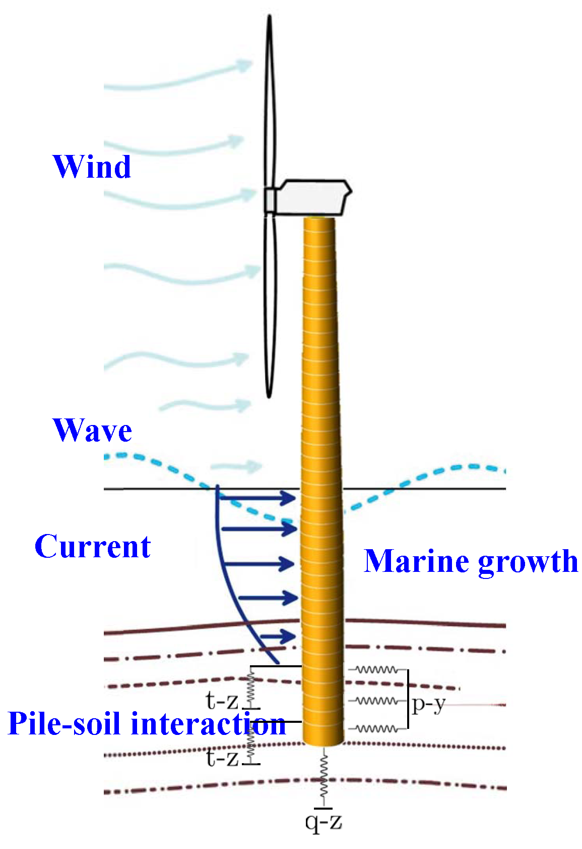
A numerical model of monopile should be established to perform the inverse evaluation procedure as a prerequisite of the optimization step. As the physical interaction between monopiles and their surroundings are incredibly complex, long and slender structures in monopiles, such as turbine foundation, tower, or blades, are always modeled as beam or bar. In contrast, flanges and other local masses are modeled as concentrated mass points.
Monopiles with different marine soils are permanently installed far offshore, where wind, wave, and current are present. The seventh-order stream function theory is used to model wave, and the current model’s standard velocity profile in IEC 61400-3-1 is used. However, wind load is not calculated here; the results provided by the wind turbine supplier are used.
As the physical properties of marine soil are highly dispersed, the soil-structure interaction of offshore wind turbines is one of the prominent sources of uncertainty in their dynamic response. This uncertainty also brings an unignorable disturbance in their condition evaluation. Currently, p-y curves in American Petroleum Institute (API) RP 2GEO (or their recently-developed modified variants, such as the PISA model [28]) and classical soil constitutive models included in commercial finite element software are commonly used. As the p-y curves are easy to implement and have lower computational costs, they are used to show the methodology proposed.
Aiming at reducing the modeling uncertainty of offshore wind turbines, the inverse evaluation method is based on the in-situ optimization of the soil-structure interaction parameters, which are one of the primary sources of uncertainties in offshore wind turbine modeling and analysis. Recently, it has been argued that the p-y curves can be rather conservative on the soil response [28]. However, the method proposed can be enlightening though the parameters may suffer from a deficiency in model assumptions.
The numerical model proposed for offshore wind turbines can be shown as
Figure 2.
Physical model for offshore wind turbines
2.3.2. Objective Function for Inverse Evaluation
This paper combines the in-situ modal identification results using structural monitoring data and numerical results obtained to form the objective function. To do this, it should be first confirmed that the modal identification results are stable over a relatively long time, such as one day (twenty-four hours). Otherwise, the objective function based on the obtained results doesn’t make sense as they vary without parameter variations.
The objective function is selected as follows.
where denotes the 2-norm, and is the first-order modal frequency obtained by the numerical model and that obtained by the monitored data, respectively. is the first-order modal results that match , defined as the minimum value satisfies
Where is the variation ratio of modal frequencies, which measures the span where the modal frequency varies, = 0.05 ∼ 0.1 (DNV-ST-0126).
Once the objective function is defined, to find the optimal value (that fits the in-situ data best), the inverse evaluation procedure should traverse as much as possible, if not all, values in the parameter space.
2.3.3. Parameter Space for Inverse Evaluation
According to the geotechnical report of the wind farm, the offshore wind turbine investigated is installed on a site with eight stratums of marine soil, with forty-two parameters comprised of nine different kinds. The soil-structure interaction parameters included are given in Table 2.
The statistical distribution of soil parameters is highly spatially discrete. Therefore, the variation of soil parameters can be assumed to follow a normal or log-normal distribution. It is assumed that the parameter X of the soil-structure interaction model in different soil layers obeys the normal distribution, with mean value as that provided by the geological survey (the value used for foundation design), , and coefficient of variation between 0 and 0.5, , that is
Where .
A screening process is first conducted to select parameters with higher single-factor sensitivity through sensitivity analysis to reduce the number of parameters for inverse optimization. Then the chosen parameters are assumed to follow the distribution defined in Eq.(14), and three to five representative values are selected randomly as the inputs for the optimization algorithm at each iteration.
2.3.4. Random Search Algorithm for Inverse Evaluation
Global optimization methods include grid search, random search, Bayesian optimization, gradient-based optimization, etc. As the efficiency of grid search is limited by the number of parameters and the values of parameters, while the Bayes optimization relies on prior information to establish the probability model of search parameters and objective function, and gradient-based optimization can quickly run into local optimization situation, a random optimization algorithm is used here for global optimization of pile-soil interaction parameters. In the meantime, the random optimization algorithm is a good choice as there are too many soil parameters whose distribution is roughly unknown, and it can also get globally optimized results in fewer iterations than grid search [29].
Given the upper and lower bounds of the parameters, the random search algorithm takes a random combination of parameter values from the interval. It carries on the parameter update during an iterative process. In addition, by designing a suitable parameter updating algorithm, the random search can overcome the limitations caused by initial parameter distribution assumptions.
The random search algorithm can be implemented using the following steps:
1. Define the objective function , penalty function , and coefficient (if used). The convergence criteria and the maximum number of iterations should also be set.
2. Determine the upper and lower bounds of the parameters , and estimate the distribution .
3. Set an initial parameter value , and solve the initial objective function value .
4. Generate m random parameter values according to parameter distribution , and solve , where . If , repeat step 4 until .
5. If there exists , set . Repeat steps 3 and 4 until the iteration reaches the convergence criteria or the maximum number of iterations. The final is the optimized parameter value under the convergence criteria or the maximum number of iterations.
The flow chart of the random search algorithm is shown in Figure 3.
Once the in-situ modal frequencies of monopiles are identified as stable, an objective function can be selected using both the numerical and modal identification results. Subsequently, inverse optimization can be performed using a random search algorithm in the assumed parameter space. The parameter results in the minimum optimization objective function are identified as the in-situ parameter of the monopile, as it can make the numerical model best approximate the in-situ structure.
3. Results and Discussion
To analyze the in-situ state of offshore wind turbines, inverse evaluation is performed here to obtain their in-situ parameters based on a random search algorithm, using numerical modal results and those identified from monitored data. Parameters used in the numerical model are given in Table 3.
The soil parameters from the geological survey are listed in Table 4 (not all).
3.1. Operational Modal Analysis
The operational modal results are first analyzed to check whether stable in-situ modal frequencies exist, as this is a prerequisite for the inverse optimization step next.
3.1.1. Verification of Stable Modes
Both SSI-COV, SSI-DATA, and N4SID are used in the operational modal identification for mutual verification. In the modal identification procedures, model order s is assumed to be 40. Modal results confirmed that model order s is suitable (results not included here). The modal convergence criteria are set to an error in modal frequency and damping ratio no greater than and , while mode shape consistency is no less than respectively.
Results obtained from different modal identification methods are shown in Figure 4. As shown, the results from N4SID are closely consistent with either SSI-COV or SSI-DATA. However, there are more modal results in SSI-COV than in SSI-DATA, which may result from differences in the solution method.
As shown in Figure 4, the Complex Mode Indicator Function (CMIF) is also used for the method verification, which is defined as [30]
Where is the k-th singular value of frequency response function (FRF) matrix at circular frequency , i.e.
Where and are the complex unitary matrices, is a rectangular diagonal matrix with non-negative real numbers on the diagonal. The diagonal entries of are uniquely determined by and are known as the singular values. The maximum of the CMIF corresponds to the characteristic frequency of the system.
As shown in Figure 4, the CMIF maxima are the same in SSI-COV and SSI-DATA results, as the FRF results obtained from structural monitoring data are identical for the same monopile. Meanwhile, the maxima of CMIF results also coincide with the N4SID results, which is evidence that the modal identification results are convincing. As the three modal identification methods gave satisfactory results here, the N4SID algorithm is used in the rest of the paper considering the benefits in computation cost and result post-processing.
To eliminate fake modes resulting from mathematical poles and determine the mode order for modal matching in the inverse evaluation, the modal assurance criterion (MAC), defined as the cross-operation results between all identified mode shape vectors, is used. MAC is defined as [31]
Where and are the mode shape with order i and j.
The first ten mode results from N4SID are shown in Table 5. The corresponding MAC results are shown in Figure 5. Multiple large non-diagonal values (greater than 0.5) appeared in the MAC results in the modal identification results, indicating the presence of n highly correlated modes. Furthermore, it can be seen from Table 5 that unstable modes with large damping ratios appear in the modal results (greater than ), which are physically unrealizable and can be considered as results from highly-correlated mode shapes. Figure 5 also shows the results with fake modes removed in (b). The corresponding MAC results are satisfactory, indicating that the correlation between each mode meets the requirements for stable modal results.
The above discussion confirmed that stable modal results can be identified and separated satisfactorily. However, as we need to use the modal results for inverse evaluation, it is necessary to check whether the modal frequencies are invariant or whether they are only engaged with slow or minor changes, i.e., approximately constant, during a relatively long time (for example, during one day).
3.1.2. Check of Stationary Modal Frequencies
According to the modal identification and verification procedures proposed above, the results at different times in a day are shown in Figure 6 (only the first ten-order results are included). Time IDs are custom labels to identify different times in a day, with no practical significance otherwise. Besides, Time IDs 1 to 4 correspond to the initial start-up of the studied wind turbine, which is unstable in its working state, while Time IDs 5 to 24 correspond to power production. To eliminate the uncertainty in the working state of the wind turbine, the discussion focuses on the results from Time ID 5 to 24 in the following.
As shown in Figure 6, the first-order modal frequencies of the offshore wind turbine during its power production are approximately constant (varying between 0.247Hz and 0.291Hz), with a median characteristic frequency of 0.274Hz repeatedly occurring at a different time in one day. However, the corresponding frequencies slightly changed at other times, with a median fluctuation range of - to compared to the characteristic frequency. Meanwhile, the damping ratios show an irregular and drastic change between 0 and .
The above results quantitatively confirmed that the first-order modal frequencies of offshore wind turbines are not a constant value during power production. However, it also confirmed that the first-order modal frequencies could be considered approximately constant here, and a first-order modal frequency Hz can be used.
A further comment should be made here. Based on the above results, it is difficult to determine whether the first-order modal frequencies still exist in whole or in part for longer periods (such as 48 hours or longer). However, it is sufficient to show the inverse evaluation method proposed. Further work is needed to reveal the modal characteristics of offshore wind turbines during the working state.
3.2. Verification of Inverse Evaluation Method
3.2.1. Selection of Sensitive Parameters
According to the geotechnical report of the wind farm, the offshore wind turbine investigated is installed on a site with eight stratums of marine soil, with forty-two parameters comprised of nine different kinds. For the convenience of parameter selection, it is temporarily assumed that the coefficient of variation is = 0.5 to screen the sensitive parameters of the soil layer.
According to the single-factor sensitivity analysis results, the soil parameters can be classified into four categories, i.e., highly sensitive, sensitive, marginally related, and uncorrelated. Selected sensitivity analysis results for the first two categories are shown in Figure 7. The rest of the sensitivity results are omitted as the idea behind the selection criterion is easy to understand. Meanwhile, as there are deficiencies in the geological measurement mechanism of some parameters that may lead to deviations in the geotechnical results, a total of 30 parameters for random search and inversion are considered here based on the sensitivity analysis.
3.2.2. Convergence Verification
Iterative optimization can be carried out by selecting all parameters (a total of forty-two) or selected sensitive parameters (a total of thirty). Considering the computing capacity of our workstation (Intel i9 12950HX, NVIDIA RTX A3000, 128 Gigabyte RAM, 2 Terabyte Solid State Disk), the maximum number of iterations is set to N=100, and the convergence criterion is set to the residual of objective function not greater than . It was found that the computation time for one parameter case can still cost approximately two to six hours.
The convergence curve of a typical calculation case is shown in Figure 8. Not all parameter cases can obtain physically meaningful results, but only valid iterations are plotted versus the residual of the objective function. As shown, the results confirm that this method can converge to a specific soil parameter combination, which is considered the actual soil parameter during the working state of the wind turbine.
3.2.3. Sensitivity Analysis of Initial Parameters
Optimization methods can be confusing if they are susceptible to initial values. To check whether the algorithm can always converge under arbitrary parameter cases, five different parameter cases are proposed to show the convergence characteristics. The convergence curves are provided in Figure 9.
As shown in Figure 9, all initial parameter cases (large objective function values corresponding to iteration number equals zero) can converge to desirable objective function values (approximately zero). Meanwhile, although the convergence rate varies with different initial parameter cases, the ideal objective function value (less than 2.0‰) can be reached in 4 iterations at least. All initial parameter cases shown can reach the convergence criterion in roughly ten iterations. Therefore, whatever the initial parameter values are, the algorithm can always converge after some iterations, corresponding to the in-situ parameter values.
The initial parameters can be considered as parameters provided for the initial design of offshore wind turbines, which are always obtained by the geotechnical report of the wind farm. As a result of poor geotechnical investigation work, these parameters are sometimes found to deviate a lot from the actual values.
The results in this subsection confirmed that whatever the provided parameters are, we can always converge to a parameter combination after some iterations using the proposed inverse evaluation algorithm. The converged results correspond to the situation that the numerical results fit the monitored results best, implying that the obtained parameters can be considered in situ.
As soil is not an ideal continuum medium, its physical properties are discrete and spatially related. Therefore, the results of a geotechnical survey are reliable only at a certain probability level. However, the results of the geotechnical survey, i.e., the initial value of the inverse evaluation procedure, are vital as they are significant input in foundation design for offshore wind turbines. It is thus necessary to evaluate whether all the possible initial parameters (obtained from a geotechnical survey) can lead to identical or close results.
3.3. Physical Characteristics of Inverse Evaluation Results
According to the inverse evaluation method, it is found that different initial parameter cases may converge to slightly different optimal parameters, i.e., multiple parameter combinations all fit the monitored results well. In reality, only one combination of parameters should exist for the in-situ parameters. Therefore, it is necessary to compare the results from different initial parameter cases to see whether the structural response is numerically similar.
Based on the in-situ monitoring data of an offshore wind farm in Jiangsu Province, China, five parameter combinations can be obtained using the proposed inverse evaluation method regarding different initial parameter cases. Using these different parameter results from the inverse evaluation method, several design targets regarding monopiles, such as axial capacities and displacements, are analyzed, and the result deviation in different results is compared. These results can be considered as the influence of initial geological parameters, which can shed some light on the impact of uncertainty in geological surveys.
3.3.1. Deviation in Axial Capacities
As the axial bearing of monopile foundations are mostly controlled by compression, their tension capacity is not discussed here. Compression capacities solved by the physical model using different inverse evaluation methods are shown in Table 6. Max. Error corresponds to maximum relative error between compression capacities.
The safety factor and UC values are also shown in Table 6, which are defined as following respectively
Where , are the maximum axial force and design capacity. According to NB/T 10105-2018 (Code for Design of Wind Turbine Foundations for Offshore Wind Power Projects) issued by the National Energy Administration of China, the ultimate axial capacity of the structure should satisfy
Where the structural importance coefficient is usually taken as 1.1.
Since the maximum axial force on the structure is far less than the design capacity, the safety factor is much larger than the importance coefficient , therefore, the difference in the design capacity results from different initial parameter cases does not cause any safety risk. However, excessive safety factor may lead to redundancy and uneconomic in materials.
As shown in Table 6, the axial capacities are different under different parameter cases, with a maximum difference at about 28%. According to the design report of the offshore wind farm, the compression capacity is 27887 kN, as the maximum compression force is 8356 kN, the compression capacity in the parameter cases can all meet the design requirements. However, the design value of compression capacity in parameter case 5 are less than the original design capacity.
The results suggest that the design axial capacities of offshore wind turbines are sensitive to geological parameters, and sufficient allowance of bearing capacity should be reserved in the design.
3.3.2. Deviation in Pile Displacements
To ensure the normal operation and power generation of offshore wind turbines, the foundation design should meet the requirements for the safe operation of wind turbines. Displacement at some positions on the turbine foundation solved by the physical model using different inverse evaluation methods is shown in Table 7, where Max. Error corresponds to the maximum relative error between the results obtained by different parameter cases. Figure 10 shows the positions where the displacements are provided.
In Table 7, there are differences in the displacement and rotation angles of the tower bottom, pile head, and pile bottom obtained from inverse evaluation method under different initial parameter cases. The maximum difference in displacement value at the tower bottom under different cases can reach about 3.42 cm, and the maximum difference in rotation angle is about 0.28 degrees. In the meantime, the maximum difference in displacement value at the pile head is about 1.80 cm, and the maximum difference in rotation angle is about 0.28 degrees. The maximum results at the pile bottom are approximately 0.68 cm and 0.01 degrees, respectively.
According to NB/T 10105-2018 (Code for Design of Wind Turbine Foundations for Offshore Wind Power Projects) issued by the National Energy Administration of China, the displacement and rotation at the tower bottom are not specially controlled. Meanwhile, neither the displacement at the pile head nor the rotation angle at the pile bottom. In accordance with the deformation control requirements for monopile foundations in the NB/T 10105-2018, the displacement at the pile head should be less than 10.8 cm, the rotation angle at the pile head should be less than 0.00436 radians (0.25 degrees), while the displacement at the pile bottom should be less than 10 mm.
According to the results in Table 7, the results can all satisfy the requirements in NB/T 10105-2018 except the X displacements at the pile head (position B in Figure 10).
The displacements are further compared with the design results in Table 8. As shown, the maximum displacements and rotation angles are all larger in the inverse evaluation results than those in the design results. These deviations are possibly because of soil stiffness distribution deviation resulting from the difference in soil parameters, as the design results are based on the parameters obtained from geological survey, while the inverse evaluation results are obtained from parameters identified from monitoring data.
The displacement and rotation angle difference in the two results show that one may underestimate the pile displacement and rotation significantly due to uncertainties in the geological survey.
3.4. Deviation versus the Design Results
To evaluate the current assumptions used in the inverse evaluation procedure, the optimal parameters obtained are introduced to the physical model proposed in Section 2.3.1. The discrepancies in the response of pile foundations between the inverse evaluation results and those of the original design are discussed in this section.
According to the assumptions used during the inverse evaluation, these optimal parameters may correspond to the in-situ parameters of offshore wind turbines. Therefore, the discrepancies in the inverse evaluation results and those of the original design can be considered issues raised by uncertainty in the design phase of the offshore wind turbines. Meanwhile, as these discrepancies resulting from input uncertainty may bring significant potential risks, they should be carefully investigated, synthesizing other information in the wind farm.
3.4.1. Discrepancy in Lateral Deflections
The lateral deflections obtained from the inverse evaluation and those of the original design are shown in Figure 11.
As shown in Figure 11, the lateral deflections of pile foundation at different elevation are roughly different from the original design results, however, though the magnitude of difference may seem to be significant, the in-situ status of the wind turbine is satisfactory as the lateral deflections are overall small, and smaller than the original design mostly, which can surely meet the requirements in the foundation design.
3.4.2. Discrepancy in Axial Deflections
The axial deflections obtained from the inverse evaluation and those of the original design are shown in Figure 12.
As shown in Figure 12, the axial deflections of pile foundations at different elevation are significantly different from the original design results. Though the trend is roughly similar, the magnitudes of maximum deflection are 0.131 cm and 0.998 cm in the original design and in-situ results, respectively. The discrepancy in axial deflection results from the difference in soil parameters. The variation in soil parameters can lead to different axial capacities. In this case, the compression capacity obtained from The inverse evaluation is 24016.8 kN, which is far below the design result (27887 kN). As a result, the axial deflection increased compared to the original design. According to NB/T 10105-2018, the in-situ status of the wind turbine is compliant with the standard as the total deflections at the pile head (pile elevation equals 0) are less than 10.8 cm.
However , as significant discrepancies in axial deflections are revealed, attention should be paid to the in-situ axial capacity and deflection of the offshore wind turbines in this wind farm. The difference indicates that the uncertainty in soil parameters can lead to significantly more considerable in-situ axial deflections than the original design results. Therefore, though the current axial deflections are acceptable, the discrepancy in the two results, i.e., the in-situ axial deflection and the original design result, implies that we should pay attention to the sensitivity of axial deflection to the soil parameters to avoid potential risks.
3.4.3. Discrepancy in Pile Rotations
The rotations obtained from the inverse evaluation and those of the original design are shown in Figure 13.
As shown in Figure 13, the pile rotations at different elevations are different but smaller from the original design results, with a maximum value of 0.00153 radians versus 0.00251 radians. However, the results are all acceptable according to NB/T 10105-2018, as all the rotation angles at the pile head (pile elevation equals 0) are less than 0.00436 radians (0.25 degrees). Meanwhile, one should notice that the difference between the two results is quite significant, with a 39.04%
3.5. Limitations of the Proposed Inverse Evaluation Method
Based on the measured results and the numerical model, we proposed a parameter inversion method for the pile-soil interaction model. This method is promising because it is straightforward to implement. However, This method is not perfect. It has several flaws itself.
First and foremost, the results obtained are related to the selected numerical model. Therefore, the proposed method can only correct the relevant parameters of the numerical model. It cannot overcome the shortcomings of the numerical model itself. A more realistic numerical model means more realistic results.
Besides, the parameter space is based on some assumptions. However, the actual distribution of the model parameters is uncertain. A more realistic parameter distribution means a faster search for real results, if any.
Finally, the calculation efficiency needs to be further improved. Surrogate models, such as the response surface model, can be considered in the next to accelerate the calculation under the premise of reliability.
4. Conclusions
Using monitoring data from an offshore wind farm in the East China Sea and numerical models, we proposed a parameter inversion method for the pile-soil interaction model based on the measured results and the numerical model. The proposed parameter inversion method comes in several steps. First, we need to construct a numerical model. Then, once the in-situ modal frequencies are identified as stable, an objective function can be selected using both the numerical and identified results. Subsequently, inverse optimization can be performed using a random search algorithm in the assumed parameter space. The parameter results in the minimum optimization objective function are identified as the in-situ parameter of the monopile, as it can make the numerical model best approximate the in-situ structure. Convergence verification results confirm that this method can converge to a specific soil parameter combination. Results also show that whatever the initial parameter values are, the proposed method can always converge after some iterations, which correspond to the in-situ parameter values. However, it was found that different initial parameter cases may converge to slightly different optimal parameters, i.e., deviations in axial capacities or pile displacements, implying the pile results are sensitive to geological parameters. Therefore, we need to make a sufficient allowance for uncertainties in geological surveys. The results obtained by the proposed method are also compared with the original design results, indicating design redundancy or risks. Though the proposed method has several flaws, it can shed some light on the influence of uncertainties in offshore wind turbines, such as soil parameters in geological surveys.
Author Contributions
Conceptualization, H.Q., W.L., and C.G.; methodology, H.Q., and C.G.; software, and validation, H.Q., and C.G.; formal analysis, and investigation, W.L.; resources, Z.J.; data curation, H.Q.; writing—original draft preparation, H.Q., and W.L.; writing—review, and editing, Z.J., and C.G.; visualization, H.Q.; supervision, Z.J., and C.G.; project administration, W.L., and Z.J.; funding acquisition, W.L., and Z.J. All authors have read, and agreed to the published version of the manuscript.
Funding
This research was supported by the National Key Research and Development Program of China (No. 2021YFF0502200), Shenzhen Science and Technology Program (No. JCYJ20220818100202006), Hong Kong Research Grants Council (No. PolyU 152634/16E and T22-502/18-R) and The Hong Kong Polytechnic University (No. 1-BBAG). The APC was funded by POWERCHINA HUADONG Engineering Corporation Limited (HDEC).
Data Availability Statement
The data is available on demand.
Conflicts of Interest
The authors declare no conflict of interest. The funders had no role in the design of the study; in the collection, analyses, or interpretation of data; in the writing of the manuscript; or in the decision to publish the results.
References
- Jahani, K.; Langlois, R.G.; Afagh, F.F. Structural dynamics of offshore Wind Turbines: A review. Ocean. Eng. 2022, 251, 111136. [Google Scholar] [CrossRef]
- Devriendt, C.; Weijtjens, W.; El-Kafafy, M.; De Sitter, G. Monitoring resonant frequencies and damping values of an offshore wind turbine in parked conditions. I Renew. Power Gener. 2014, 8, 433–441. [Google Scholar] [CrossRef]
- Häckell, M.W.; Rolfes, R. Monitoring a 5 MW offshore wind energy converter—Condition parameters and triangulation based extraction of modal parameters. Mech. Syst. Signal Process. 2013, 40, 322–343. [Google Scholar] [CrossRef]
- Devriendt, C.; Magalhães, F.; Weijtjens, W.; De Sitter, G.; Cunha, Á.; Guillaume, P. Structural health monitoring of offshore wind turbines using automated operational modal analysis. Struct. Health Monit. 2014, 13, 644–659. [Google Scholar] [CrossRef]
- Xu, M.; Au, F.T.; Wang, S.; Wang, Z.; Peng, Q.; Tian, H. Dynamic response analysis of a real-world operating offshore wind turbine under earthquake excitations. Ocean. Eng. 2022, 266, 112791. [Google Scholar] [CrossRef]
- Koukoura, C.; Natarajan, A.; Vesth, A. Identification of support structure damping of a full scale offshore wind turbine in normal operation. Renew. Energy 2015, 81, 882–895. [Google Scholar] [CrossRef]
- Chen, B.; Zhang, Z.; Hua, X.; Basu, B.; Nielsen, S.R. Identification of aerodynamic damping in wind turbines using time-frequency analysis. Mech. Syst. Signal Process. 2017, 91, 198–214. [Google Scholar] [CrossRef]
- Bajrić, A.; Høgsberg, J.; Rüdinger, F. Evaluation of damping estimates by automated operational modal analysis for offshore wind turbine tower vibrations. Renew. Energy 2018, 116, 153–163. [Google Scholar] [CrossRef]
- van Vondelen, A.A.; Navalkar, S.T.; Iliopoulos, A.; van der Hoek, D.C.; van Wingerden, J.W. Damping identification of offshore wind turbines using operational modal analysis: a review. Wind. Energy Sci. 2022, 7, 161–184. [Google Scholar] [CrossRef]
- Dong, X.; Lian, J.; Wang, H.; Yu, T.; Zhao, Y. Structural vibration monitoring and operational modal analysis of offshore wind turbine structure. Ocean. Eng. 2018, 150, 280–297. [Google Scholar] [CrossRef]
- Oliveira, G.; Magalhães, F.; Cunha, Á.; Caetano, E. Vibration-based damage detection in a wind turbine using 1 year of data. Struct. Control. Health Monit. 2018, 25, e2238. [Google Scholar] [CrossRef]
- Dong, X.; Lian, J.; Yang, M.; Wang, H. Operational modal identification of offshore wind turbine structure based on modified stochastic subspace identification method considering harmonic interference. J. Renew. Sustain. Energy 2014, 6, 033128. [Google Scholar] [CrossRef]
- Liu, F.; Gao, S.; Tian, Z.; Liu, D. A new time-frequency analysis method based on single mode function decomposition for offshore wind turbines. Mar. Struct. 2020, 72, 102782. [Google Scholar] [CrossRef]
- Liu, F.; Gao, S.; Han, H.; Tian, Z.; Liu, P. Interference reduction of high-energy noise for modal parameter identification of offshore wind turbines based on iterative signal extraction. Ocean. Eng. 2019, 183, 372–383. [Google Scholar] [CrossRef]
- Martinez-Luengo, M.; Shafiee, M.; Kolios, A. Data management for structural integrity assessment of offshore wind turbine support structures: data cleansing and missing data imputation. Ocean. Eng. 2019, 173, 867–883. [Google Scholar] [CrossRef]
- Qiu, Y.; Feng, Y.; Infield, D. Fault diagnosis of wind turbine with SCADA alarms based multidimensional information processing method. Renew. Energy 2020, 145, 1923–1931. [Google Scholar] [CrossRef]
- Iliopoulos, A.; Shirzadeh, R.; Weijtjens, W.; Guillaume, P.; Van Hemelrijck, D.; Devriendt, C. A modal decomposition and expansion approach for prediction of dynamic responses on a monopile offshore wind turbine using a limited number of vibration sensors. Mech. Syst. Signal Process. 2016, 68, 84–104. [Google Scholar] [CrossRef]
- Maes, K.; Iliopoulos, A.; Weijtjens, W.; Devriendt, C.; Lombaert, G. Dynamic strain estimation for fatigue assessment of an offshore monopile wind turbine using filtering and modal expansion algorithms. Mech. Syst. Signal Process. 2016, 76, 592–611. [Google Scholar] [CrossRef]
- Nabiyan, M.S.; Khoshnoudian, F.; Moaveni, B.; Ebrahimian, H. Mechanics-based model updating for identification and virtual sensing of an offshore wind turbine using sparse measurements. Struct. Control. Health Monit. 2021, 28, e2647. [Google Scholar] [CrossRef]
- Bisoi, S.; Haldar, S. Design of monopile supported offshore wind turbine in clay considering dynamic soil–structure-interaction. Soil Dyn. Earthq. Eng. 2015, 73, 103–117. [Google Scholar] [CrossRef]
- Arany, L.; Bhattacharya, S.; Adhikari, S.; Hogan, S.; Macdonald, J.H.G. An analytical model to predict the natural frequency of offshore wind turbines on three-spring flexible foundations using two different beam models. Soil Dyn. Earthq. Eng. 2015, 74, 40–45. [Google Scholar] [CrossRef]
- Zania, V. Natural vibration frequency and damping of slender structures founded on monopiles. Soil Dyn. Earthq. Eng. 2014, 59, 8–20. [Google Scholar] [CrossRef]
- Peeters, B.; Roeck, G.D. Reference-based stochastic subspace identification for output-only modal analysis. Mech. Syst. Signal Process. 1999, 13, 855–878. [Google Scholar] [CrossRef]
- Reynders, E. System identification methods for operational modal analysis: review and comparison. Arch. Comput. Methods Eng. 2012, 19, 51–124. [Google Scholar] [CrossRef]
- Overschee, P.; Moor, B. Subspace identification for linear systems: Theory—Implementation—Applications; Springer Science & Business Media, 2012.
- Van Overschee, P.; De Moor, B. N4SID: Subspace algorithms for the identification of combined deterministic-stochastic systems. Automatica 1994, 30, 75–93. [Google Scholar] [CrossRef]
- Verhaegen, M. Identification of the deterministic part of MIMO state space models given in innovations form from input-output data. Automatica 1994, 30, 61–74. [Google Scholar] [CrossRef]
- Burd, H.J.; Beuckelaers, W.J.A.P.; Byrne, B.W.; Gavin, K.G.; Houlsby, G.T.; Igoe, D.J.P.; Jardine, R.J.; Martin, C.M.; McAdam, R.A.; Wood, A.M.; Potts, D.M.; Gretlund, J.S.; Taborda, D.M.G.; Zdravković, L. New data analysis methods for instrumented medium-scale monopile field tests. Géotechnique 2020, 70, 961–969. [Google Scholar] [CrossRef]
- Bergstra, J.; Bengio, Y. Random search for hyper-parameter optimization. J. Mach. Learn. Res. 2012, 13. [Google Scholar]
- Peeters, B.; De Roeck, G. Stochastic system identification for operational modal analysis: a review. J. Dyn. Syst. Meas. Control. 2001, 123, 659–667. [Google Scholar] [CrossRef]
- Alvin, K.; Robertson, A.; Reich, G.; Park, K. Structural system identification: From reality to models. Comput. Struct. 2003, 81, 1149–1176. [Google Scholar] [CrossRef]
Figure 1.
Acceleration sensors on the tower: (a) Front view. (b) Top View of section A-A.
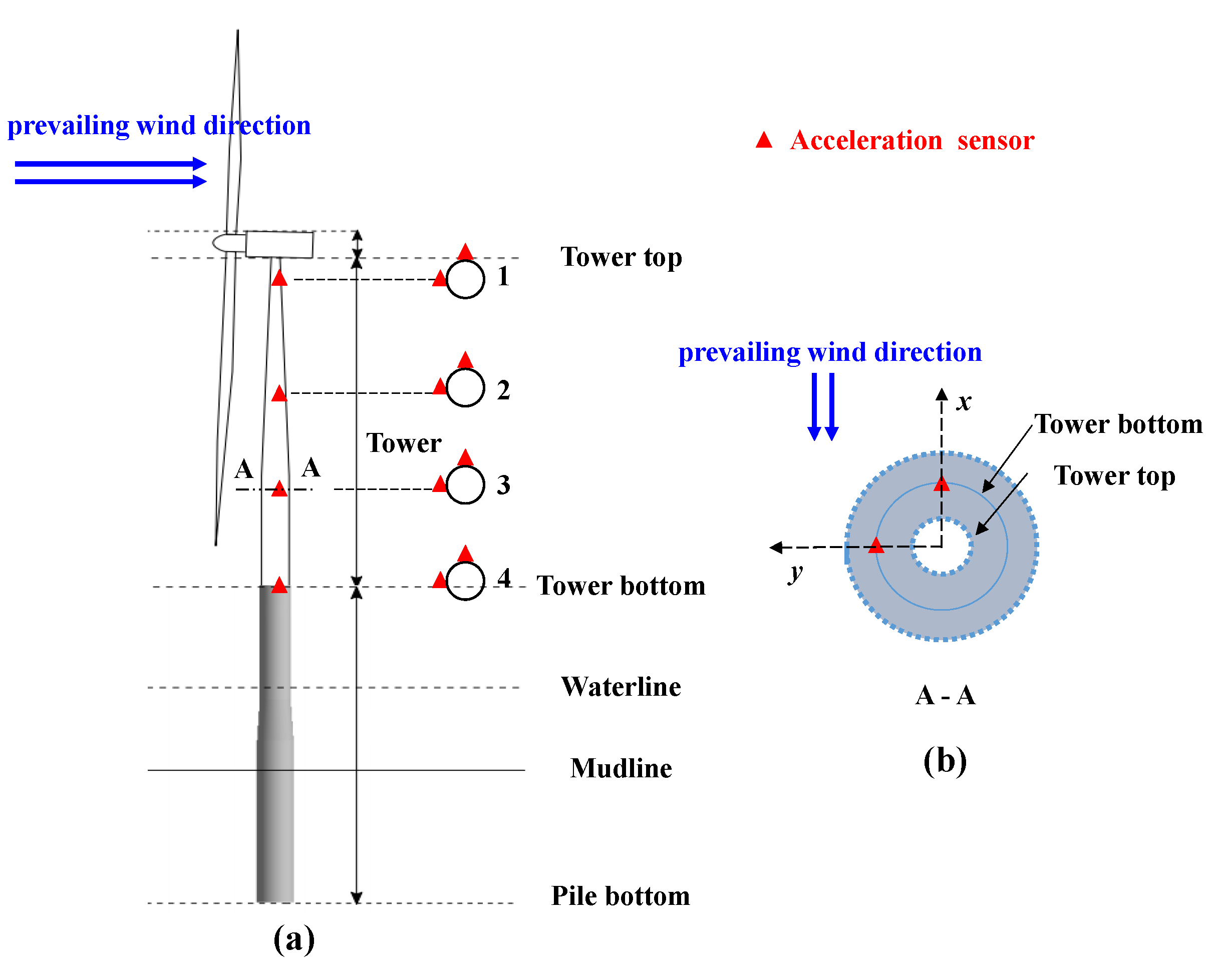
Figure 3.
Flow chart of the random search algorithm.
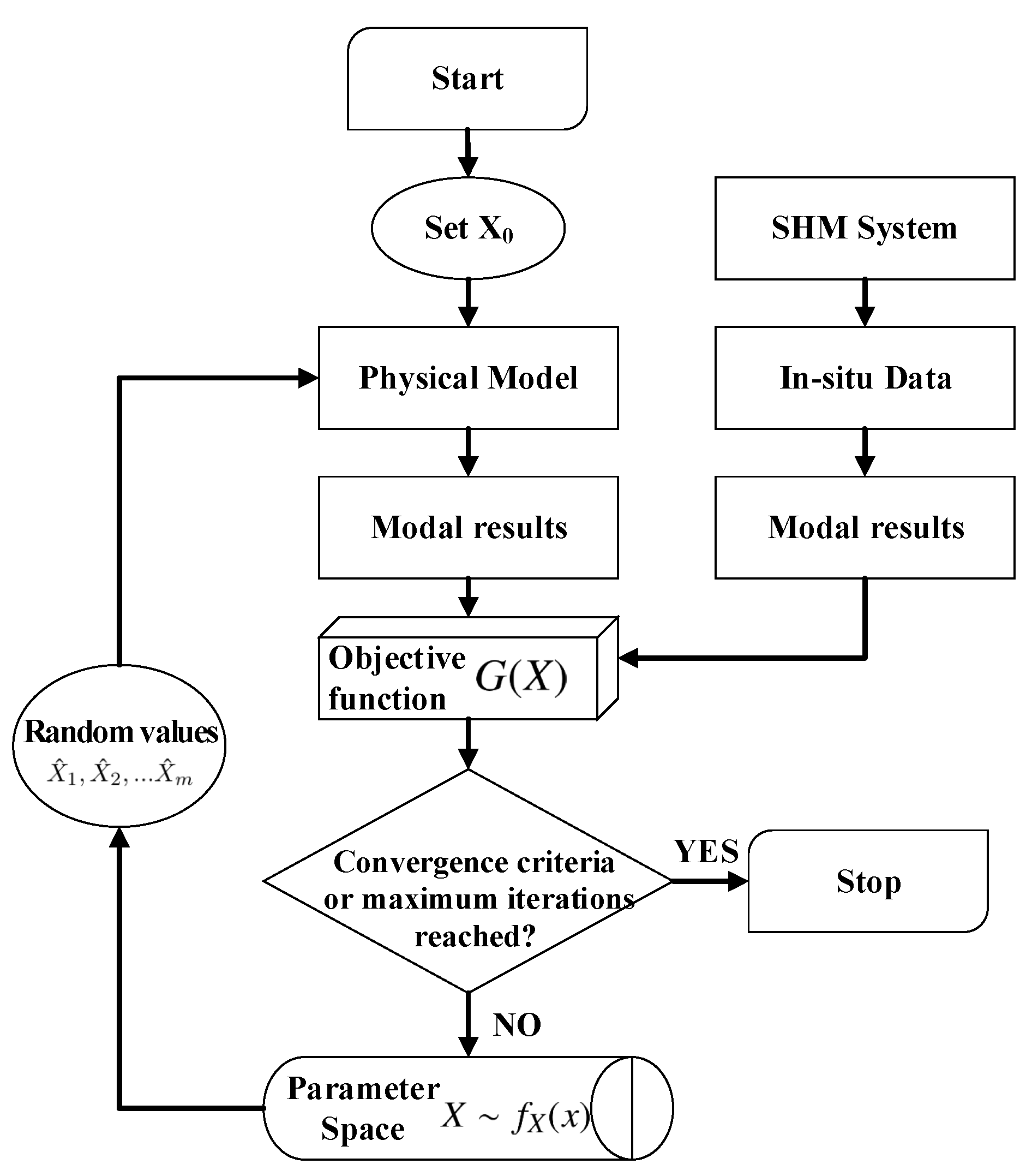
Figure 4.
Results from different methods. (a) SSI-COV. (b) SSI-DATA. The vertical dashed line shows N4SID results. ∘ and × correspond to stable or unstable modal results (poles).
Figure 4.
Results from different methods. (a) SSI-COV. (b) SSI-DATA. The vertical dashed line shows N4SID results. ∘ and × correspond to stable or unstable modal results (poles).
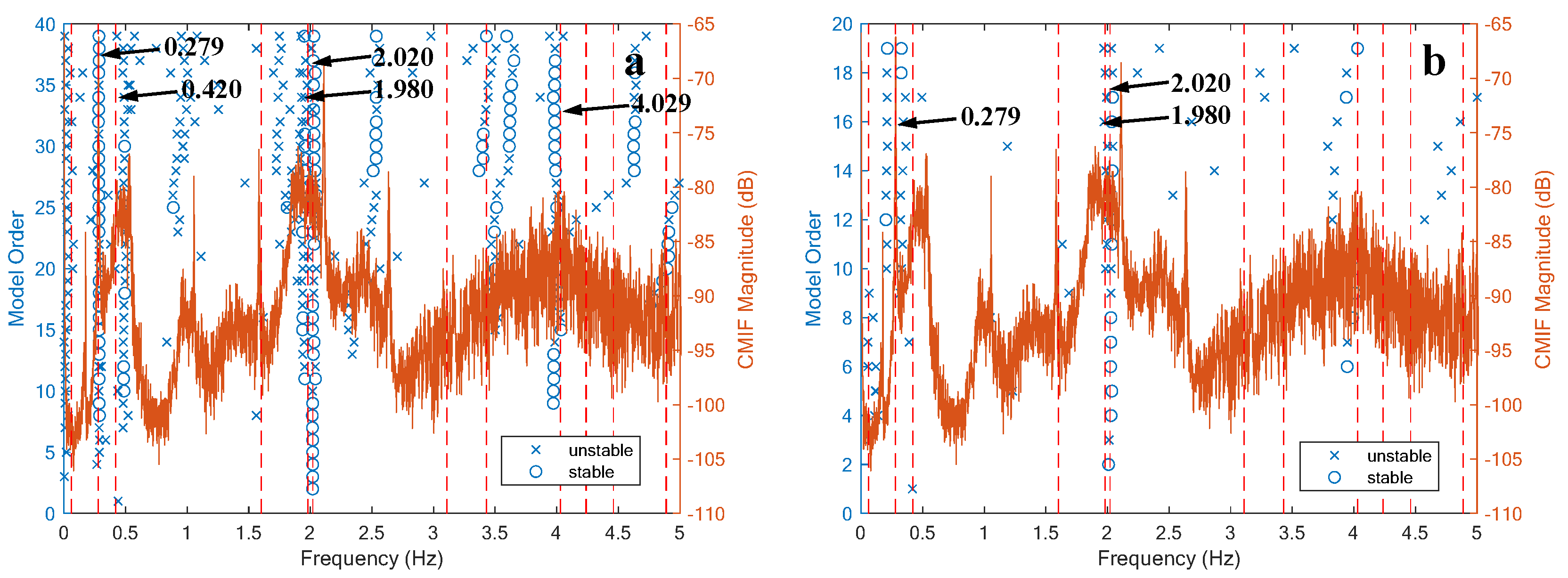
Figure 5.
MAC results of first ten identified modal results. (a) Original results. (b) Fake modes removed.
Figure 5.
MAC results of first ten identified modal results. (a) Original results. (b) Fake modes removed.
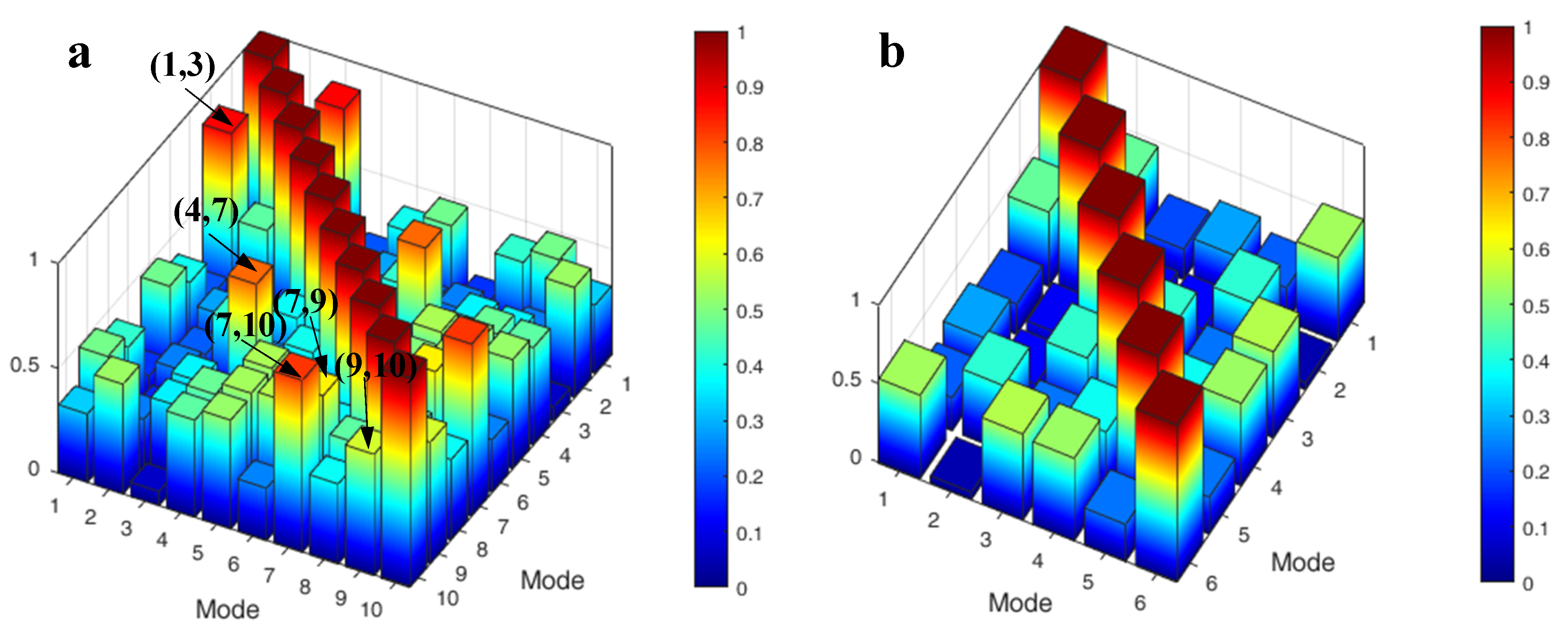
Figure 6.
Modal frequencies at different times (Time IDs) in a day. (a) Modal frequencies. (b) Damping ratios.
Figure 6.
Modal frequencies at different times (Time IDs) in a day. (a) Modal frequencies. (b) Damping ratios.
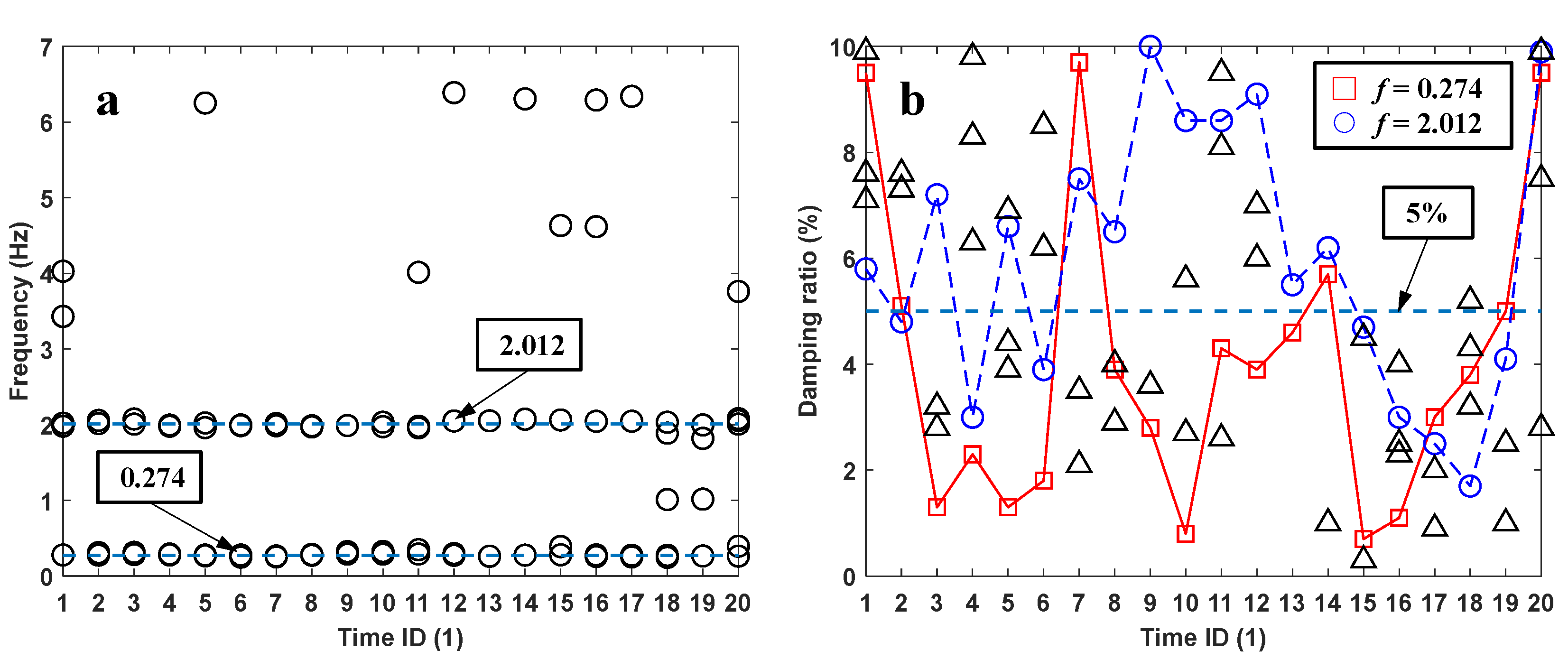
Figure 7.
Sensitivity analysis results of selected soil parameters (for illustration only). (a) Internal friction angle. (b) Effective weight.
Figure 7.
Sensitivity analysis results of selected soil parameters (for illustration only). (a) Internal friction angle. (b) Effective weight.
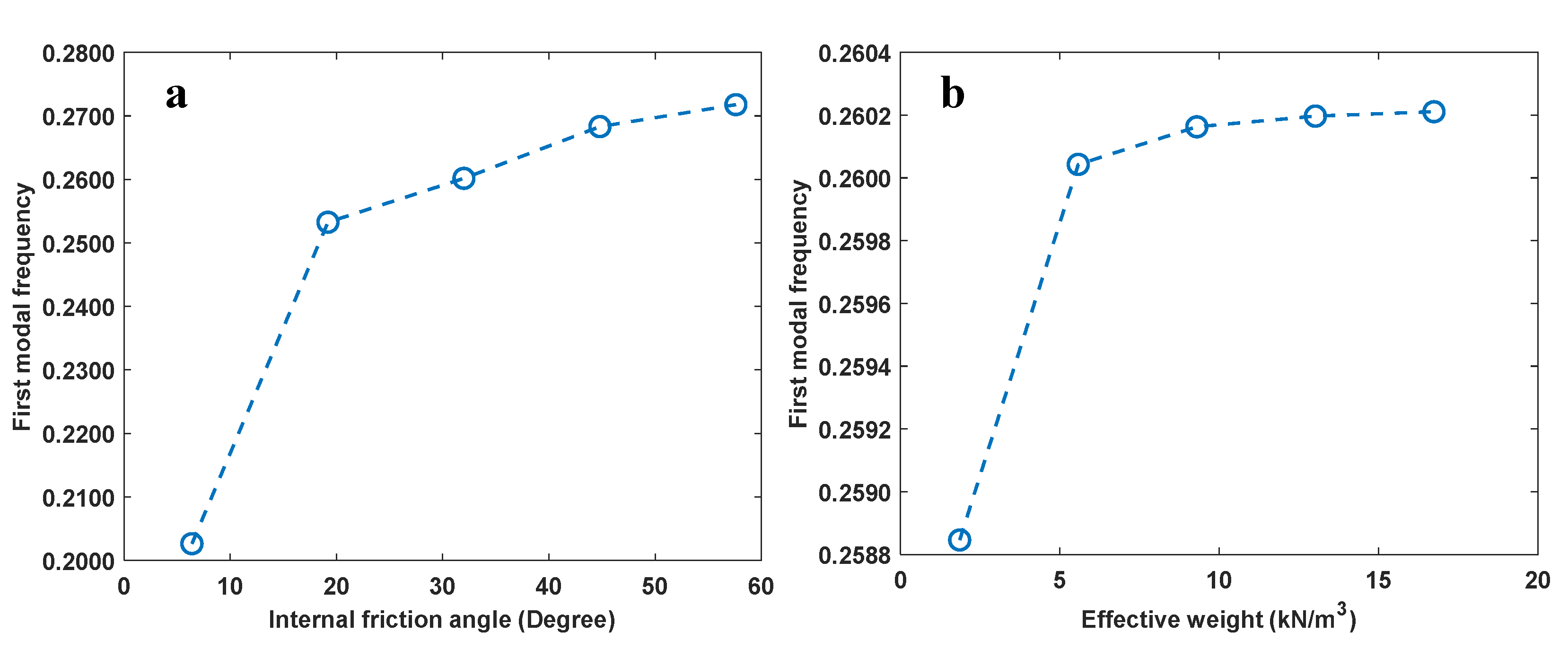
Figure 8.
Convergence curve of a typical calculation case.
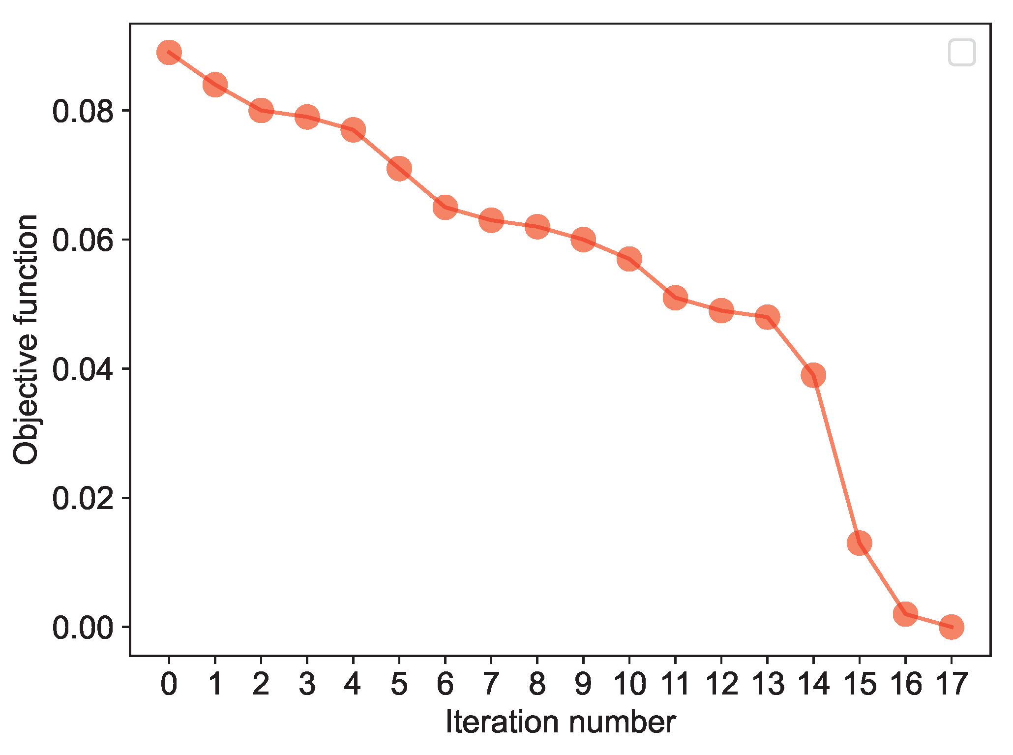
Figure 9.
Convergence curves of different initial parameter cases. Case 1 and 2 correspond to different initial parameter combinations, and corresponds to the standard deviation of the parameters.
Figure 9.
Convergence curves of different initial parameter cases. Case 1 and 2 correspond to different initial parameter combinations, and corresponds to the standard deviation of the parameters.
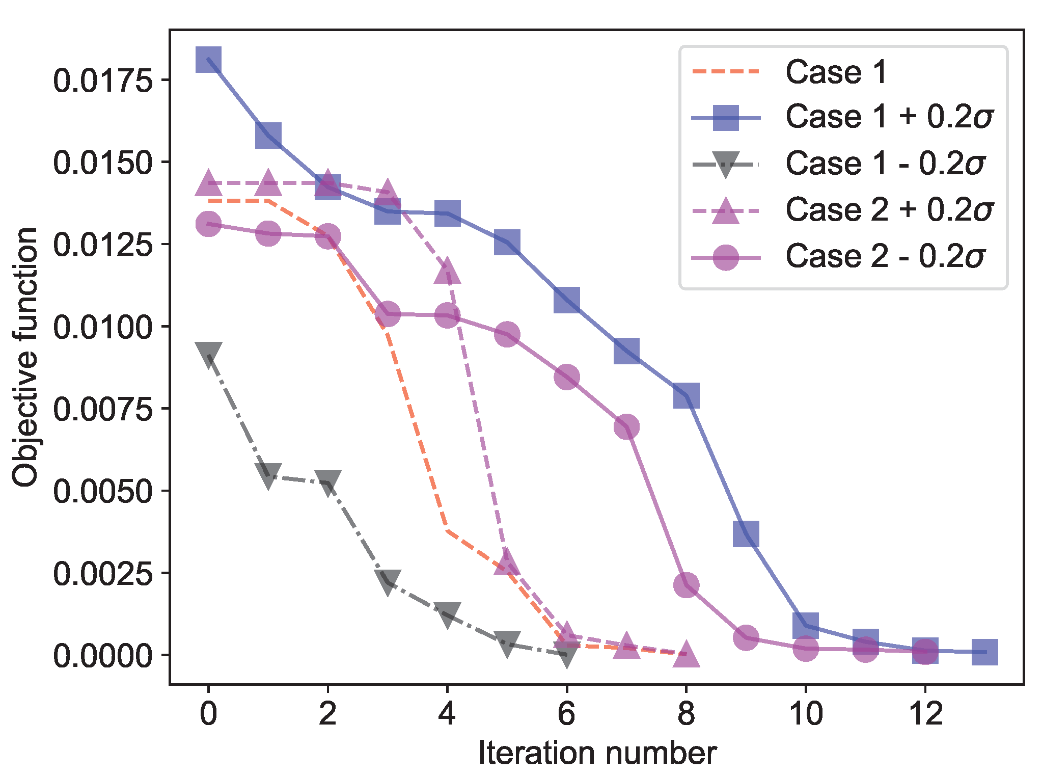
Figure 10.
Schematic diagram of positions where displacements are obtained on offshore wind turbines.
Figure 10.
Schematic diagram of positions where displacements are obtained on offshore wind turbines.
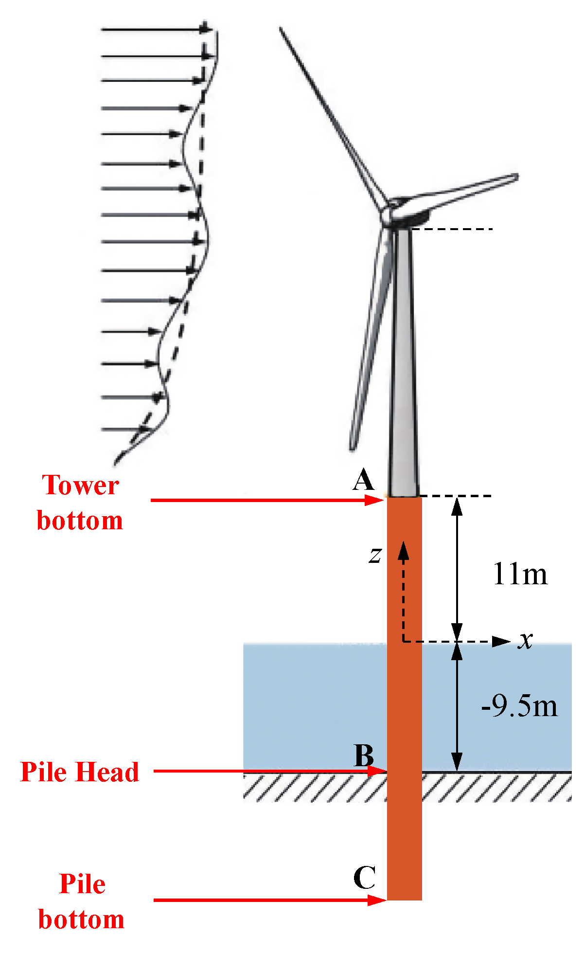
Figure 11.
Discrepancy in lateral deflections at different pile evaluations.
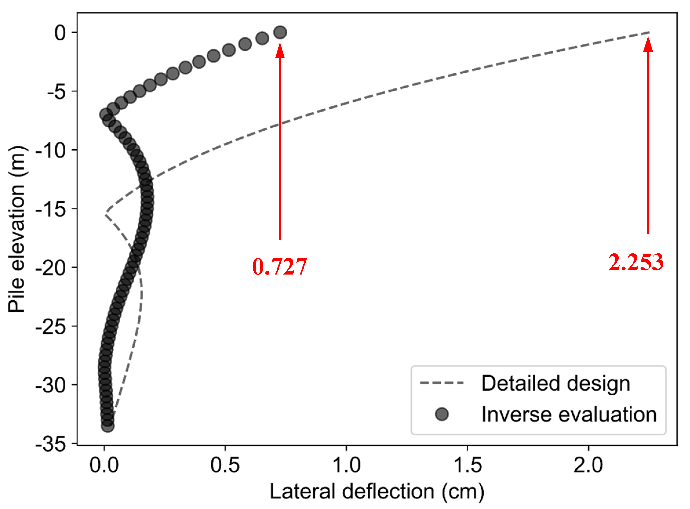
Figure 12.
Discrepancy in axial deflections at different pile evaluations.
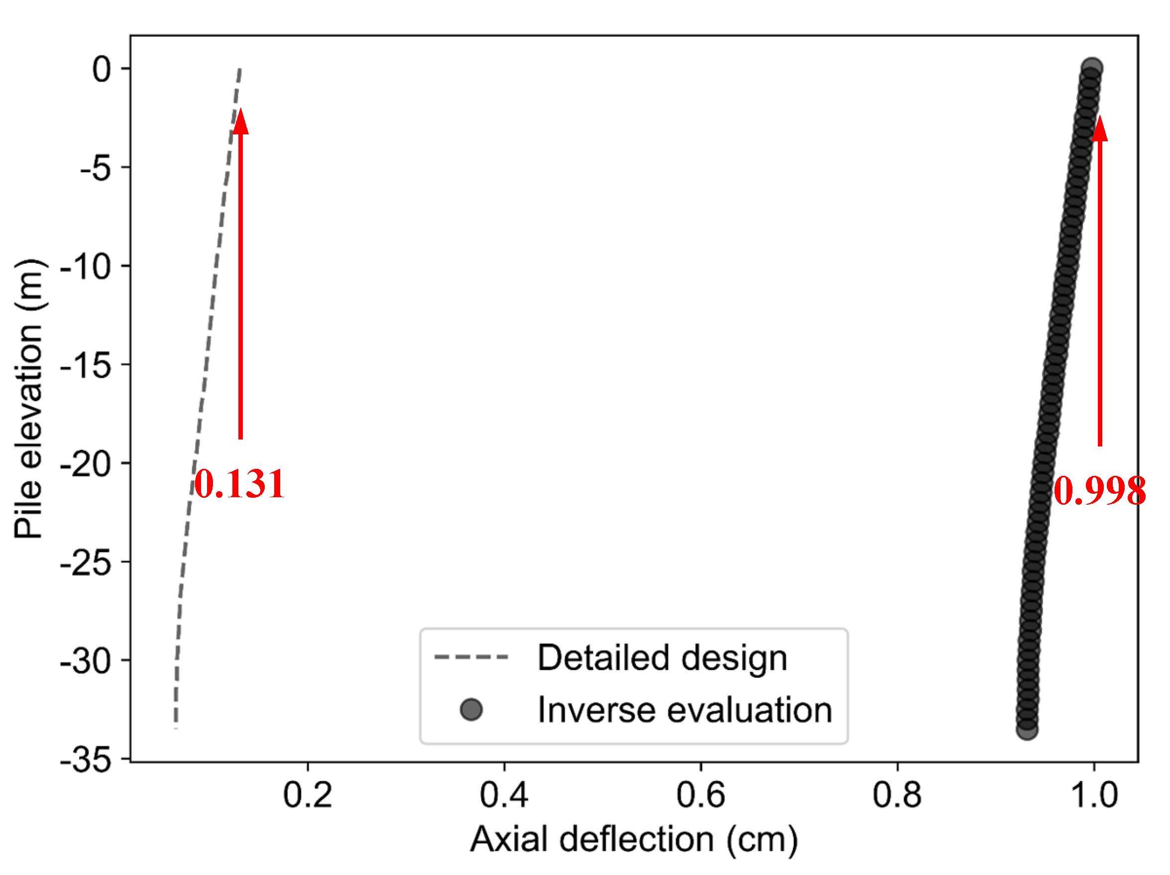
Figure 13.
Discrepancy in pile rotations at different pile evaluations.
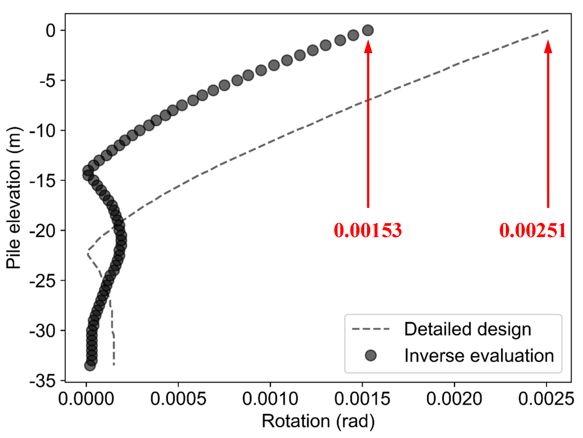

Table 1.
Acceleration monitoring points (elevation : m, acceleration : m/).
| Location | Sensor ID | Elevation | Direction 1 |
|---|---|---|---|
| 1 | J1 | 88m | X |
| 1 | J2 | 88m | Y |
| 2 | J3 | 60m | X |
| 2 | J4 | 60m | Y |
| 3 | J5 | 32m | X |
| 3 | J6 | 32m | Y |
| 4 | J7 | 12m | X |
| 4 | J8 | 12m | Y |
1 X-direction: prevailing wind direction, Y-direction: vertical to prevailing wind direction.
Table 2.
Pile-soil interaction parameters for offshore wind turbines (API).
| Parameters | Units | |
|---|---|---|
| Effective weight | kN/ | |
| Sand | Internal friction angle | Degree |
| Relative density | / | |
| Pile-soil friction angle | Degree | |
| Ultimate value of pile side friction resistance | kPa | |
| Bearing capacity factor | / | |
| Ultimate axial capacities of unit pile end | kPa | |
| Clay | Undrained shear strength | kPa |
| / |
Table 3.
Parameters used in the numerical model.
| Value | Units | Description | |
|---|---|---|---|
| Rated capacity | 4.5 | MW | Variable-pitch variable-speed |
| Drag coefficient | 1.2 | / | Marine growth included |
| Inertia coefficient | 2.0 | / | Marine growth included |
| Marine growth thickness | 10 | cm | / |
| 50 year return wave height | 3.35 | m | / |
| 50 year return wave period | 4.75 | s | / |
| Bottom velocity | 2.310 | m/s | / |
| Pile diameter | 5.5 | m | / |
| Mudline level | -9.5 | m | Scour included |
Table 4.
Parameters for the offshore wind turbine installation site.
| Stratums | |||||||||
|---|---|---|---|---|---|---|---|---|---|
| silt | 8.5 | 28 | 0.2 | 23 | 75 | / | / | / | / |
| silt | 9.3 | 32 | 0.35 | 27 | 87 | / | / | / | / |
| silt | 9.4 | 33 | 0.4 | 28 | 87 | / | / | / | / |
| clay | 9.2 | / | / | / | / | / | / | 60 | 0.008 |
| clay | 8.4 | / | / | / | / | / | / | 40 | 0.015 |
| sand | 9.6 | 34 | 0.45 | 29 | 93 | 36 | 8640 | / | / |
| sand | 9.9 | 35 | 0.5 | 30 | 96 | 40 | 9600 | / | / |
| sand | 9.9 | 36 | 0.6 | 31 | 99 | 42 | 10080 | / | / |
Table 5.
Modal results obtained by N4SID (first ten order).
| Order | 1 | 2 | 3 | 4 | 5 | 6 | 7 | 8 | 9 | 10 |
|---|---|---|---|---|---|---|---|---|---|---|
| Frequency | 0.060 | 0.279 | 0.420 | 1.603 | 1.980 | 2.020 | 3.108 | 3.431 | 4.029 | 4.238 |
| Damping ratio | 1.000 | 0.095 | 0.152 | 1.000 | 0.099 | 0.058 | 0.469 | 0.076 | 0.071 | 0.447 |
| Type | × | ∘ | × | × | ∘ | ∘ | × | ∘ | ∘ | × |
Table 6.
Comparison of compression capacity under different initial parameter cases (kN).
| Case 1 | Case 2 | Case 3 | Case 4 | Case 5 | Max. Error | |
|---|---|---|---|---|---|---|
| Design Capacity | -30286.2 | -28012 | -32881.8 | -30557.5 | -23787 | -27.66% |
| Maximum force | -8356 | -8356 | -8356 | -8356 | -8356 | 00.00% |
| Safety factor | 3.624 | 3.352 | 3.935 | 3.657 | 2.847 | 38.23% |
| UC | 0.276 | 0.298 | 0.254 | 0.273 | 0.351 | 38.23% |
Table 7.
Comparison of displacement (cm) and rotation angle (degree) under different initial parameter cases.
Table 7.
Comparison of displacement (cm) and rotation angle (degree) under different initial parameter cases.
| Case 1 | Case 2 | Case 3 | Case 4 | Case 5 | Max. Error | |
|---|---|---|---|---|---|---|
| X displacement at A | 11.8456 | 14.3527 | 10.9306 | 11.6138 | 12.2302 | 31.31% |
| Z displacement at A | -0.8512 | -0.9111 | -0.7912 | -0.8441 | -1.0713 | -26.14% |
| Y rotation angle at A | 0.3255 | 0.3534 | 0.3080 | 0.3149 | 0.3327 | 14.75% |
| Z rotation angle at A | 0.0026 | 0.0026 | 0.0026 | 0.0026 | 0.0026 | 0.00% |
| X displacement at B | 2.6962 | 4.2020 | 2.4049 | 2.8400 | 2.8201 | 74.73% |
| Z displacement at B | -0.8018 | -0.8617 | -0.7418 | -0.7947 | -1.0219 | -27.40% |
| Y rotation angle at B | 0.1728 | 0.2008 | 0.1554 | 0.1623 | 0.1801 | 29.23% |
| Z rotation angle at B | 0.0023 | 0.0023 | 0.0023 | 0.0023 | 0.0023 | 0.00% |
| X displacement at C | 0.7350 | 0.7920 | 0.6800 | 0.7290 | 0.9460 | 39.12% |
| Y displacement at C | 0.7840 | 0.4080 | 0.1390 | 0.1800 | 0.8190 | 489.21% |
| Z displacement at C | 0.7840 | 0.4080 | 0.1390 | 0.1800 | 0.8190 | 489.21% |
| Y rotation angle at C | 0.0034 | 0.0126 | 0.0103 | 0.0023 | 0.0034 | 450.00% |
| Z rotation angle at C | 0.0034 | 0.0126 | 0.0103 | 0.0023 | 0.0034 | 450.00% |
Table 8.
Comparison of maximum displacement (cm) and rotation angle (degree) between different initial parameter cases and the design values.
Table 8.
Comparison of maximum displacement (cm) and rotation angle (degree) between different initial parameter cases and the design values.
| Case 1 | Case 2 | Case 3 | Case 4 | Case 5 | Design values | |
|---|---|---|---|---|---|---|
| Displacement at A | 11.8456 | 14.3527 | 10.9306 | 11.6138 | 12.2302 | 10.36 |
| Rotation at A | 0.3255 | 0.3534 | 0.3080 | 0.3149 | 0.3327 | 0.2962 |
| Displacement at B | 2.6962 | 4.2020 | 2.4049 | 2.8400 | 2.8201 | 2.25 |
| Rotation at B | 0.1728 | 0.2008 | 0.1554 | 0.1623 | 0.1801 | 0.1438 |
| Displacement at C | 0.7840 | 0.7920 | 0.6800 | 0.7290 | 0.9460 | 0.25 |
Disclaimer/Publisher’s Note: The statements, opinions and data contained in all publications are solely those of the individual author(s) and contributor(s) and not of MDPI and/or the editor(s). MDPI and/or the editor(s) disclaim responsibility for any injury to people or property resulting from any ideas, methods, instructions or products referred to in the content. |
© 2023 by the authors. Licensee MDPI, Basel, Switzerland. This article is an open access article distributed under the terms and conditions of the Creative Commons Attribution (CC BY) license (http://creativecommons.org/licenses/by/4.0/).
Copyright: This open access article is published under a Creative Commons CC BY 4.0 license, which permit the free download, distribution, and reuse, provided that the author and preprint are cited in any reuse.


