1. Introduction
The concept of Industry 4.0, also known as the Fourth Industrial Revolution, emerged as a strategic initiative launched at the 2011 in the Hanover Fair by the German Government within the "High-Tech Strategy 2020 Action Plan" [
1] which an association of businessmen, politicians, and academics promoted a new approach aimed at empowering and transforming the German manufacturing industry through the use of cyber-physical systems (CPS), Internet of Things (IoT) and cloud computing [
2]. Since then, this term has evolved, encompassing increasingly diverse interpretations, perspectives, and concepts, although it has a common element to all of them, “smart manufacturing” consisting of digital manufacturing, digital-networked manufacturing, and intelligent/smart manufacturing [
3].
To a relevant extent, this development is determined by the use of cyber-physical systems and although there are many definitions [
4,
5,
6,
7], all of them are characterized by the integration or collaboration of computer systems with physical systems (mechanical, electrical and/or human) to perform a specific function (communication and/or control) and perform real-time calculations (analysis). Their use in industrial environments requires capturing, processing, analyzing, and storing enormous amounts of data.
Industry 4.0 revolutionizes manufacturing by increasing flexibility, mass customization, quality, and productivity through the introduction of the nine pillars: IIoT (Industrial internet of things), Big Data, horizontal and vertical integration, simulations, cloud, augmented reality, autonomous robots, 3D printing, and cybersecurity: The use of high technology implies changes in the management of organizations, including policies and strategies within assets maintenance [
8]. Furthermore, [
9] indicate that intelligent maintenance within Industry 4.0 is oriented towards self-learning, failure prediction, diagnosis, and triggering maintenance programs, and [
10] indicate the suitability of its use, since the use of supervised models for making forecasts will ensure that the process operates correctly and efficiently without incurring high maintenance costs and reducing product quality degradation.
2. Description of the equipment, facilities, and data.
This paper addresses the prediction of the behavior of a hydrogen compressor in the petrochemical industry, specifically in the production of caprolactam used in the manufacture of nylon 6 fibers. The compressor is used to compress hydrogen from 0.35 kg/cm² to 285 kg/cm² in a multi-stage process where the hydrogen is compressed and cooled in four stages in order to keep it below 150 ºC (423 K).
The current level of preventive maintenance corresponds to level 3 according to [
11] since there is a monitoring and alarm system that alerts operators if any anomalies occur, in addition to performing the mandatory preventive maintenance every three months. The objective is to employ Industry 4.0 technologies with the purpose of increasing maintenance up to level 4, relying on real-time data monitoring based on predictive techniques. Knowledge acquisition takes place through the training of a neural network that uses self-attention mechanisms to determine the hyperparameter configuration that best fits the type of data generated by the equipment. Due to the enormous volume of real-time sensor data generated in facility operations, a highly specialized distribution control system is implemented to enable efficient analysis and decision-making.
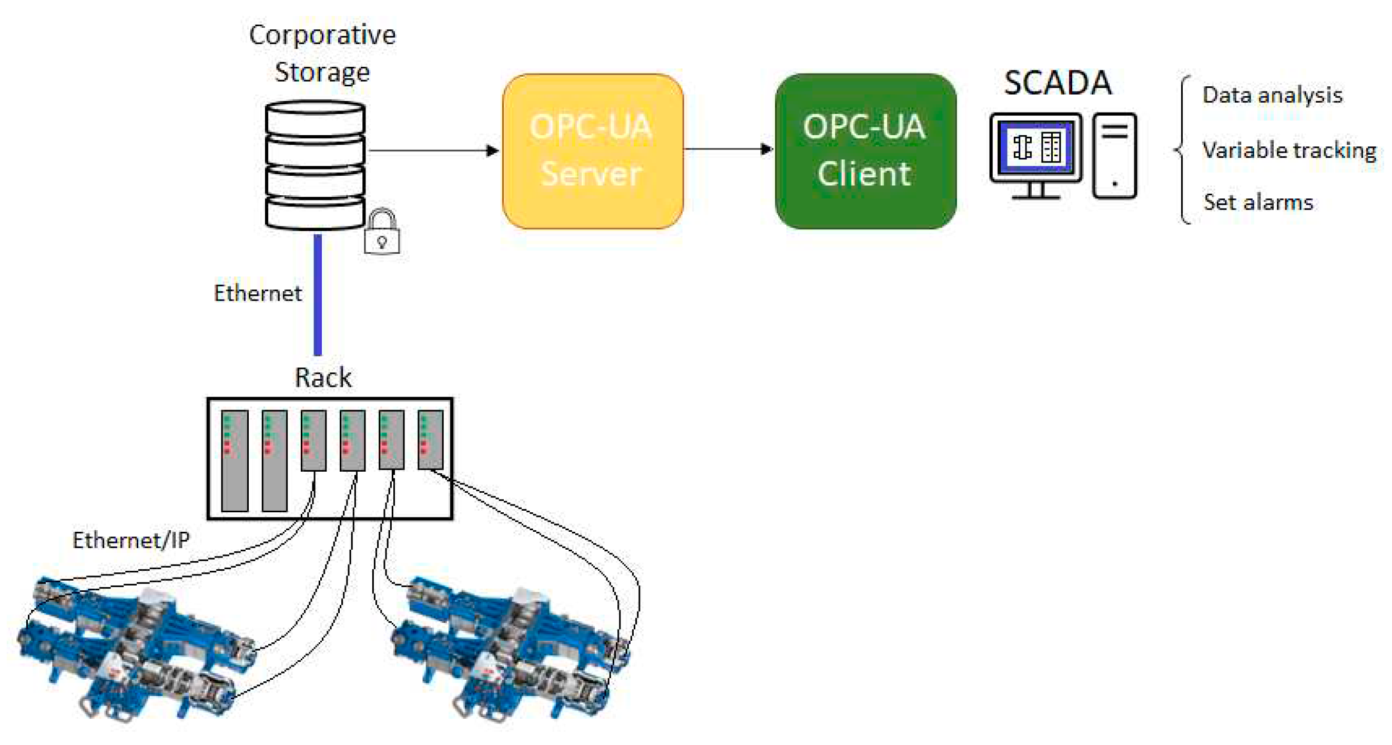
Figure 1 shows how data is collected through the asset's sensors and connects via Ethernet to the control racks, which in turn send the signal to the unique data base which share the data through the OPC-UA server for subsequent processing by users. In the absence of a fog layer, raw sensor data are transmitted directly to clients who process monitoring in real-time through a SCADA system, and adjust variable values as needed to prevent out-of-range operating situations. Materials and Methods should be described with sufficient details to allow others to replicate and build on the published results. Please note that the publication of your manuscript implicates that you must make all materials, data, computer code, and protocols associated with the publication available to readers. Please disclose at the submission stage any restrictions on the availability of materials or information. New methods and protocols should be described in detail while well-established methods can be briefly described and appropriately cited.
The equipment generates data points every single minute, with the output pressure nominally set at 285 kg/cm² and controlled within limits of 265 and 305 kg/cm². With the object of predicting its operation on an hourly basis, these limits must be adjusted to match new average values. Applying the central limit theorem, the new limits are established at 282.5 and 287.5 kg/cm² using the expression σ= (305-265)/(6√60) to estimate the new standard deviation, thus the new limits control will be set at ±3 σ.
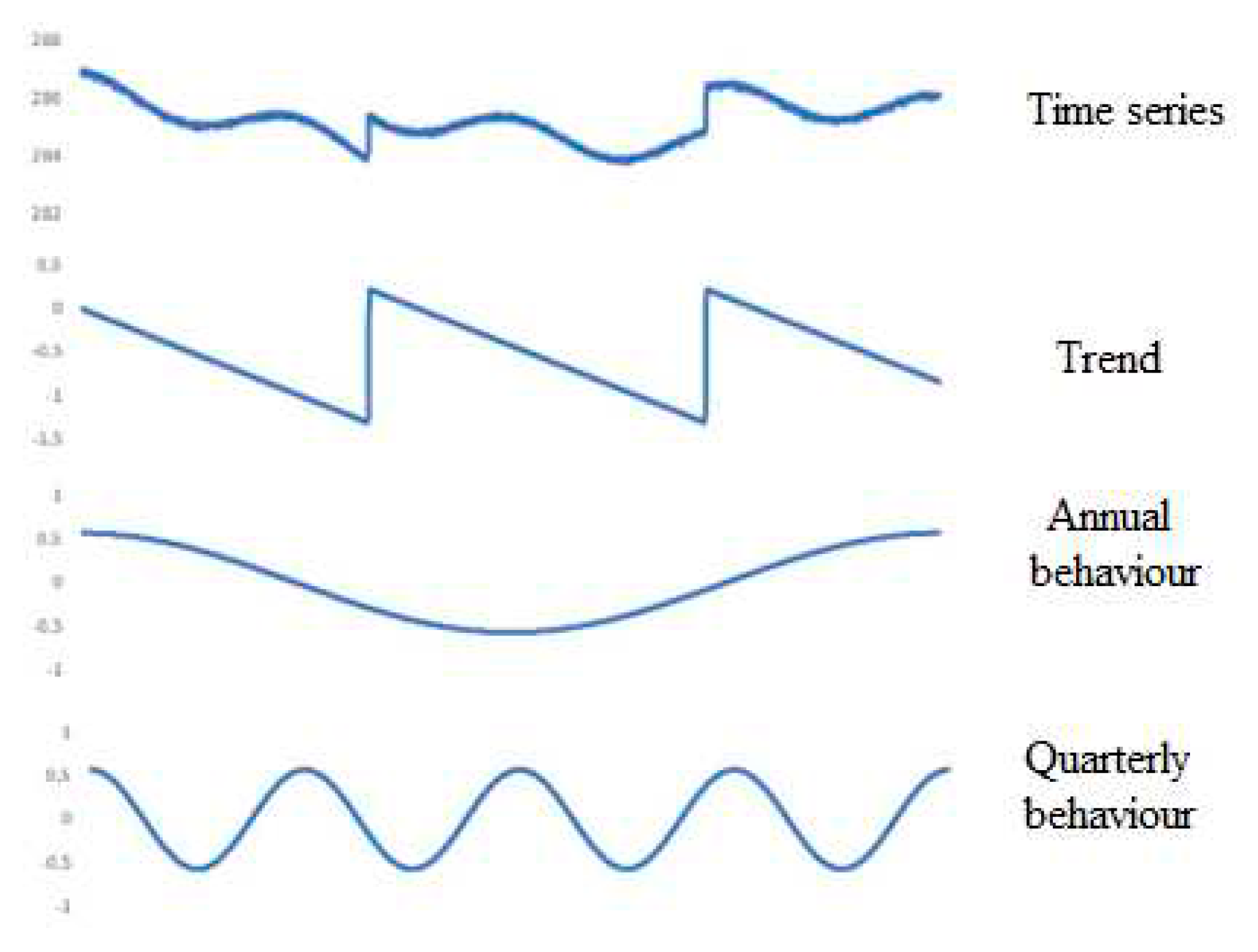
The time series have been created by generating pseudorandom numbers and using sine functions to generate seasonal behaviors, thus as shown in
Figure 2, the data used have been created from a series composition, consisting of a trend, two cyclical components (annual and quarterly), and noise.
Trend shape depicts an imbalance in the compressor that reduces the outlet pressure over time and a manual adjustment by the control room operator is required no achieve the nominal value again. Annual and quarterly series aim to symbolize the regular fluctuations due to changes in the environment (ambient pressure and temperature) that affect the normal operation of the equipment. The final model includes a noise part consisting of a normal distribution N(0, 0.032), in order to incorporate an hourly variation component into the process, that is to say 0.25σ of the minutely variation of the data.
3. Neural network with self-attention.
Originally designed for natural language processing, the network of (Vaswani et al., 2017) known as Transformer uses only attention mechanisms to predict the output sequence, instead using LSTM networks along with attention mechanisms of type [
12] or [
13] as was previously utilized. The novel approach of Transformers uses three types of attention architectures: self-attention of the input data in the encoder, masked attention of the sequences it should predict in the decoder, and finally, cross-attention, where the information from the encoders and that contained in the decoder, specifically from masked attention, is integrated.
We use a model inspired by [
14] to capture dependencies between separate points in the sequence, although instead of using all parts of the Transformer network, including encoders and decoders, to predict the behavior of time series values, only the self-attention mechanism of the encoder is used along a feed-forward layer to obtain the output tensor. The attention block uses three independent networks: query (Q), key (K), and value (V) to acquire information from input data and obtain a proper representation of the data. For each attention head, the layer calculates the attention weight through the dot product between query and key vectors divided by a scaling factor (d) and transformed by the softmax function (Equation 1).
The attended output of each attention head is used to compute a weighted sum of the value vectors. In the end, all attended outputs from all attention heads are concatenated linearly to obtain the final output of each attention head.
The additional utilization of convolutional networks is commonly used in data from numerical series, due to the high feature extraction capability. [
15] indicate that a convolutional network is a type of dense, feed-forward neural network has successfully applied in many dominions such classification problems or time series classification [
16]. Its structure allows the model recognizes specific patterns and abstract information from the input sequence.
Additionally, [
17] described the batch normalization as a regularization technique that is applied to input layers consisting of normalizing the activation values of the units in that layer so there is a mean of 0 and a standard deviation of 1, which improves stability and facilities convergence speed while avoiding problems such as exploding or vanishing gradients. Do not confuse batch normalization with input data normalization, which involves scaling input data to a specific range to improve numerical representation.
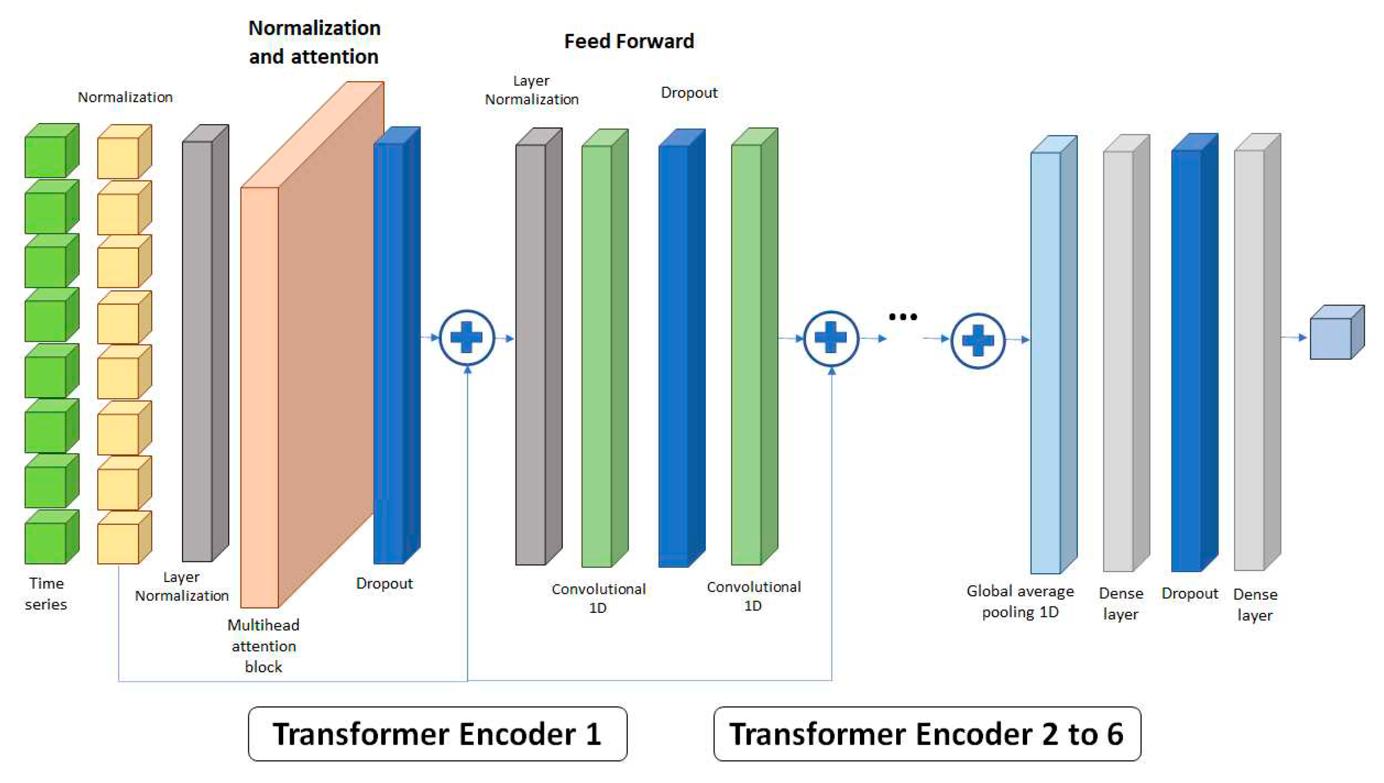
At the output of the encoders a Global average polling 1D layer (GAP1D) is added for polling and preserving all relevant information in a single layer that can straightforwardly understood by single or multiple dense layers. Thus,
Figure 3 shows the network used, in which the normalized sequence of data to be predicted is introduced into a normalization layer prior to its entry into the multi-head attention block, and a dropout layer is applied to its output [
18] to prevent excessive overfitting of the model. This set of layers and blocks forms the normalization and multi-head attention block. The obtained vectors are added to the normalized input sequence and introduced into the Feed Forward layers, which consist of a normalization layer, a dropout layer, and two 1D convolutional layers, and finally, adding the output to the input of this layer, thus forming the encoder structure. This architecture can be repeated up to six times in succession, although in this study, the maximum number of encoders used is four. The output of the network is formed by a GAP1D, and to conclude, the information passes through the dense layer equipped with another dropout layer to obtain the time series forecast.
4. Results
4.1. Design of experiments and response surface method.
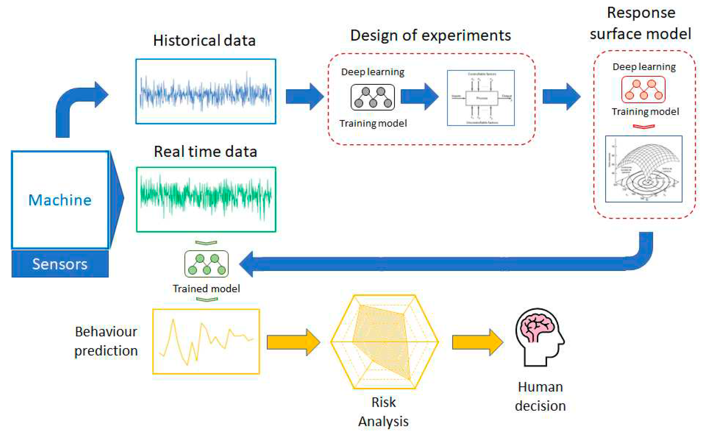
The flowchart followed in this methodology is shown in
Figure 4, where, based on historical data, the value of the hyperparameters is simultaneously modified to determine which ones are significant in the performance of the network, attempting to minimize their output, in this case the mean absolute error (MAE), defined by
, where y
t is the true output, ŷ
t is the estimation and T the number of data points. The design of experiments (DoE) size depends on the quantity of hyperparameters, so in many times some type of reduction has to be selected to reduce the number of runs and save computing time. Once the factors that significantly affect the output variable are known, a response surface model is applied in order to determine which factors, or their interactions are relevant in the network performance and whether the point of minimizing the error can be determined.
To reduce the computational requirements of the hardware, relevant hyperparameters are adjusted at the optimal point, while irrelevant factors are tuned to their lowest values. The neural network is then trained using historical data while new data are collected from the compressor and the model makes a prediction showing a time series. Based on training and predicted data, and their experience, the control room technicians analyze the consequences of the potential equipment out-of-range operability or unplanned stoppages and then make decisions according to operational procedures. Moreover, the hyperparameters or factors considered in the study to determine the optimal size of the network that minimizes the prediction error for the supplied data are collected on
Table 1, note that they are presented normalized and encoded with -1 and 1.
Sequence size (A): indicates the number of data point from the temporal sequence that will be used in the network training to obtain the forecast. Head size (B): refers to the number of neurons that are part of each head. Number of heads (C): is the number of hidden neural networks inside the transformer block. Feed Forward dimension (D): number of the 1D convolutional layers. No. encoders blocks (E): is the number of encoders that forms the network. mlp units (multi-layer perceptron units - F): is the number of neurons that compose the dense network and mlp dropout (G): is the dropout probability of the dense layer. Dropout (H): Percentage of disconnected nodes during training at the output of the attention block. Finally, the learning rate (I) determines the step size at each iteration while moving towards a minimum of a loss function.
Due to the high number of factors being considered, 9, the use of a fractional factorial design is deemed necessary. The resolution of the design depends on the number of runs desired and the level of aliasing that is acceptable among the factors and their second, third, or higher-order interactions. Thus, III is the smallest possible resolution for obtaining a screening of the most relevant attributes [
19]. In accordance with the aforementioned assumptions, the
is the design that best fits the premises with a 2
5 reduction, although there is aliasing between the factors and second-order interactions. As a result of the chosen design, only 2
4 (16) trials need to be conducted instead of the 512 initially considered in the model. Since a replication is performed to improve the error estimation, a total of 32 runs are finally executed. In
Appendix A, the
Table A1 with the conducted experiment and the RSM are included on
Table A2, showing the obtained MAE and the number of trained parameters by the neural network.
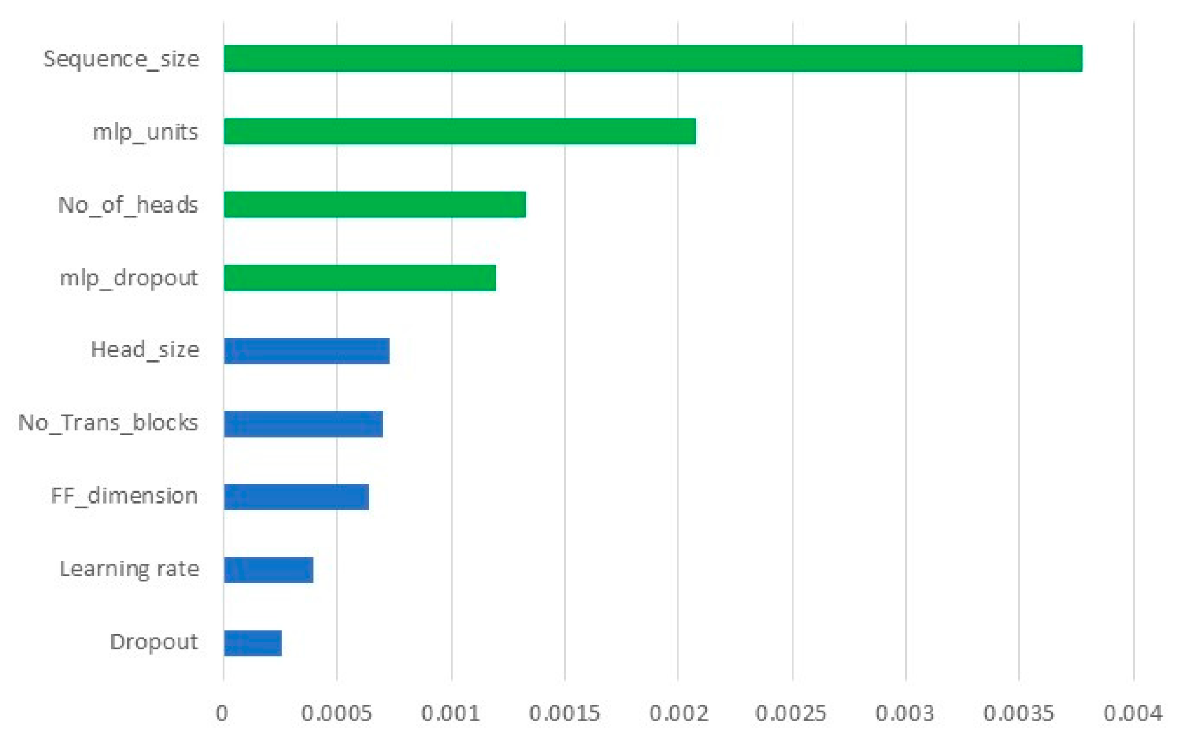
From the experiment, two relevant values are obtained: the MAE and the number of trainable parameters for each run, and
Figure 5 shows the absolute value of the coefficients of the normalized variables, with green indicating variables whose t-test is significant. Hence, four of the attributes were found to be significant: data sequence size, number of neurons of the dense layer, number of heads, and dropout of the dense network.
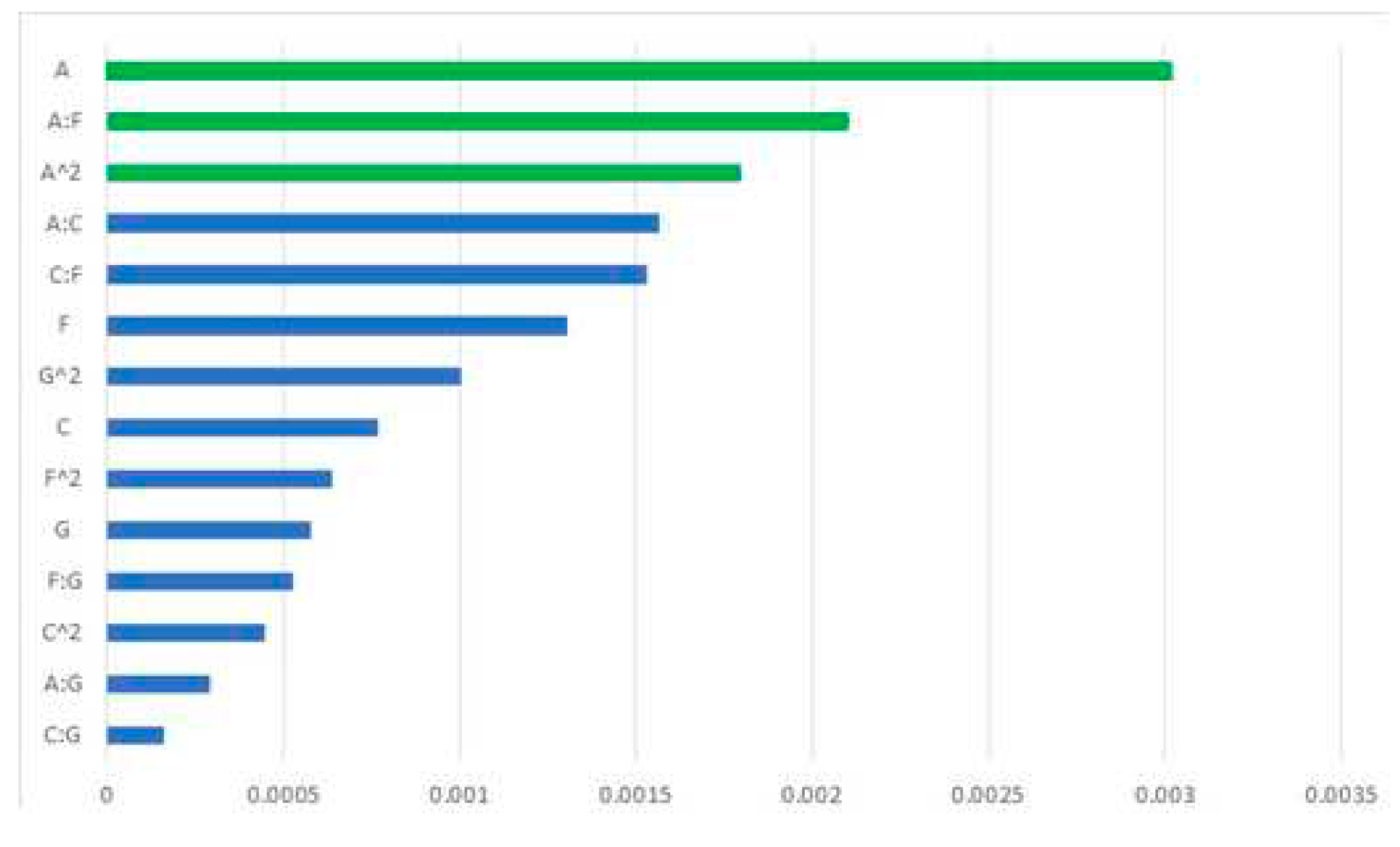
The Box-Behnken’s response surface model only employs those four factors, with the aim of its use being twofold: to recognize the optimal operating point of the neural network that minimizes prediction error and to identify the existence of significative second-order interactions. The RSM performs 24 runs to which 7 replications are added around the central point to be able to include curvature in the model and a replica is performed.
Figure 6 represents the Pareto chart of the absolute value of the coefficients of the normalized variables and their second-order interactions, whose t-test is significant (green). The lowest MAE depends on the size of the input sequence and the interaction between the input sequence size and the number of neurons in the dense output layer. Specifically, increasing the number of neurons in the output layer can lead to a decrease in the size of the input sequence, and vice versa. The equation that estimates the MAE based on the value of the normalized significant variables is ŷ = 0.037736 – 0.003021A – 0.002103AF + 0.001795 A².
4.2. Neural network complexity.
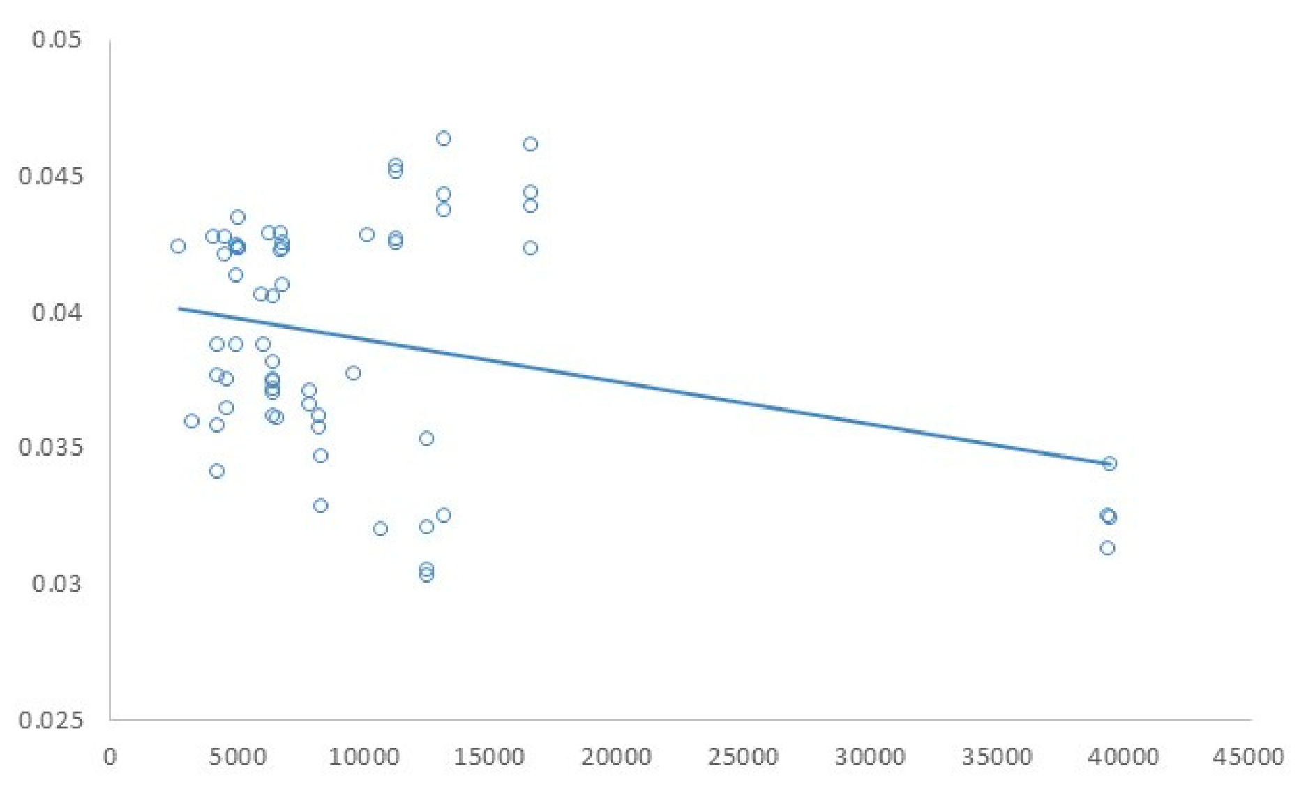
Thanks to performing a large number of trials, abundant data is available relating to prediction error and network size, allowing the study of whether the use of complex models enables improved network performance or not. The relationship between the number of trained parameters and the obtained MAE is shown in the scatter plot in
Figure 7, conducting a linear regression to determine if there is any kind of linkage between them.
Surprisingly, the F-test of overall significance of the linear regression model indicates that both of two variables are independent, therefore we cannot conclude that regression coefficient is different from 0 which implies that the complexity of the network is not related to a reduction in the prediction error, thus more complex models do not necessarily provide better estimations. The number of trained parameters depends on the values of hyperparameters related to network size such as, number of encoders, blocks, neurons, and input sequence size, while others such as learning rate or dropout do not affect to the computational burden on the hardware. The results show that simple models in terms of the number of blocks, heads per block, and number of encoders exhibit good results, reducing computational effort and training time.
The RSM estimates the stationary point of the response surface in (A=3.754, C=-5.547, F=0.985, G=1.019), and since it is out of the range of some factors and not all factors are significant, A=1 and F=0.985 are considered, yielding an estimated mean absolute error of ŷ = 0.0344. An extremely complex model is not necessary, and only 8 921 parameters need to be trained, that corresponds to sequence size (35), head size (64), no. of heads (2), feed forward dimension (2), no. encoders blocks (2), and multi-layer perceptron units (128 rounded). Nothing has been mentioned regarding dropout or learning rate, which can be adjusted to their minimum chosen values since it does not affect the network architecture; however, to avoid overfitting or slow convergence, they have been set to average values.
Just after training the model, a comparison can be made between the test data and those predicted by the neural network, as shown in
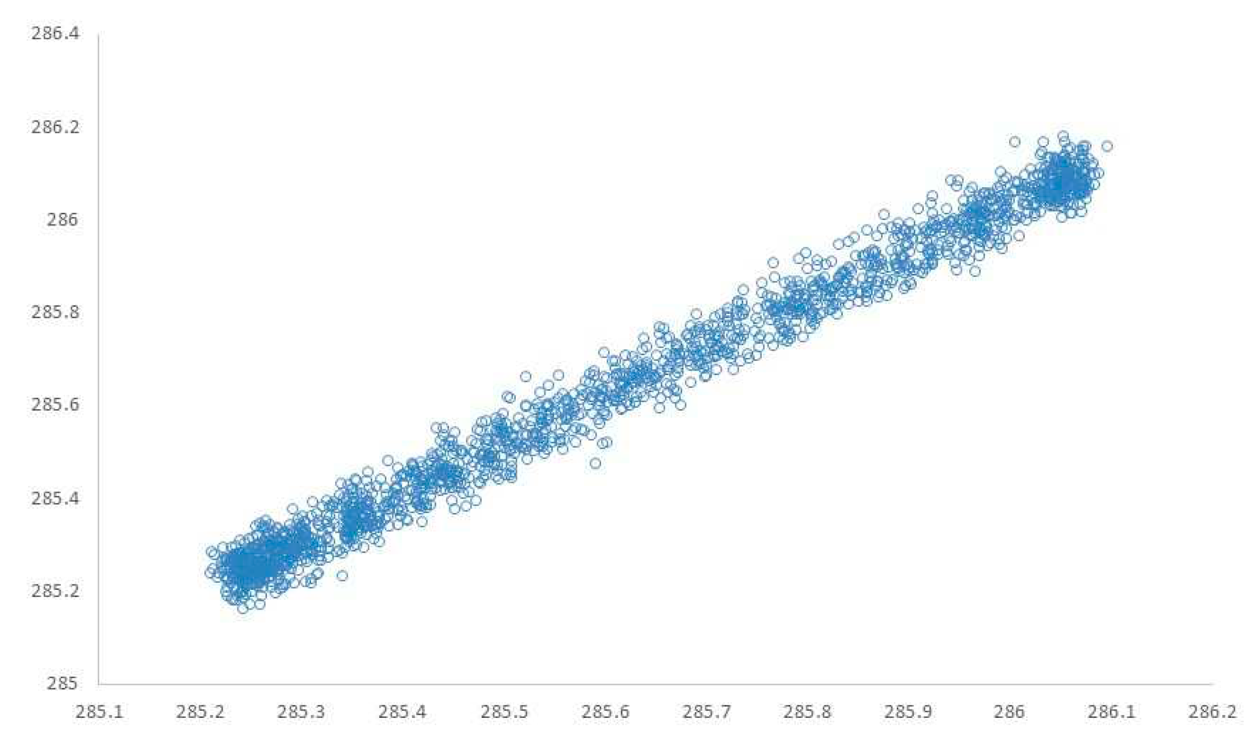
Figure 8, where a very good similarity between both types of data can be observed. We perform a regression analysis to determine the linear relationship between these values to discover whether a hidden structure exists or if we should use a simpler model.
Clearly, the linear relationship between the test and estimated data can be noticed in
Figure 9, which is why the regression line can be easily estimated, emphasizing the adjusted R² parameter, which has a value of 0.9833, indicating that the regression model is capable of predicting adequately based on the test data. The equation line is ŷ = 15.0910 + 0.9471x and the estimation of the residual standard error follows a normal distribution with mean 0 and standard deviation of 0.03669. In this case, the whole neural network can be replaced by a linear regression.
4.3. Statistical analysis.
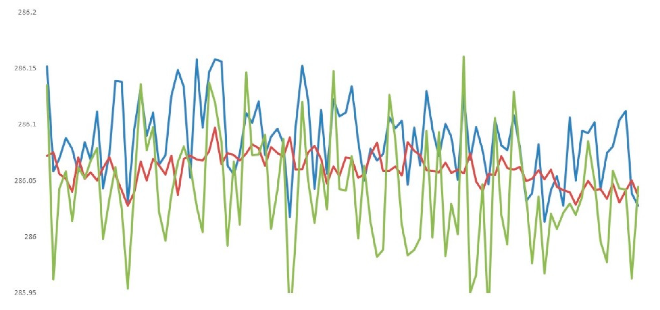
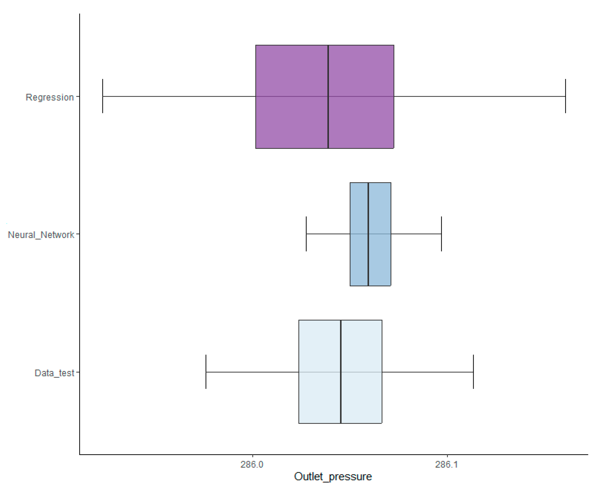
There are three types of data available for comparison, the test data, those obtained from the neural network, and from the regression model, each presenting different characteristics as shown in
Figure 10.
Multiple statistical tests are conducted to determine the normality of the data (Shapiro – Wilk) and tests of equality of means (ANOVA) and variances (Bartlett’s test), and if any of them emerge different, post-hoc analyses are performed to determine which group of data differs significantly from the others.
From
Figure 10 and
Table 2, it can be easily inferred that the different data predictions have different characteristics and although they all are normally distributed, both the mean and variance tests are significant, since the null hypothesis is rejected, marking a difference between them. The post-hoc Tukey’s test indicates that there is a difference between the means of the series, except for the mean of the original data test series and the mean of the data generated by linear regression. With respect to variance, the paired tests with Bonferroni correction for the Bartlett test indicate that all variances differ from each other, unable to affirm equality between any of them as shown on
Table 3.
From the above results, none of the series generated by the models fit the initial test data as in
Figure 10, where data test (blue line), neural network prediction (red line), and regression forecast (green line) are shown. This is where directors, supervisors, and people in charge should intervene to decide regarding their utilization, specifically if they prefer type I or type II errors occur. A simple description of both types of errors consists of the former not providing alarm signals when the equipment is truly malfunctioning, while the latter will provide failure signals when the compressor operates correctly. The neural network will generate type I errors and regression of type II.
Although all the series have different variance, the fact that the original time series and the data provided by the regression have the same mean does not imply that they should be discarded.
Figure 10.
Bloxplot comparing several data sources.
Figure 10.
Bloxplot comparing several data sources.
The final consideration is the interconnection of the data generated by the model and the control system. Due to the continuous nature of the manufacturing process and the high cost of a stoppage, the connection of the prediction model with the control system of the installation is not considered. As indicated in
Figure 4, the final decision about the prediction data point and what to do belongs to the technicians of the control room.
5. Conclusions
Although it may seem counterintuitive, the use of more complex neural networks does not necessarily produce better results in terms of minimizing the prediction error in time series. Therefore, technicians and managers should not rush into the generation and design of intricated models with the aim of obtaining better predictions. For the given data and defined network, the most important hyperparameters are the length of the input sequence to the network and the dense layer size at the output. The longer the sequence, the lower error, but at the same time, if long sequences are used to provide information, the size of the dense layers at the output of the network can be reduced.
Due to the linear relationship between the test data and those provided by the neural network, the prediction model can be simpler by employing just a model based on linear regression, where the independent variable is the data provided by the compressor and the dependent variable is the prediction. Considering that the responses of both models differ from the original data, either one can be selected, depending on the type of error that is wanted to commit in the prediction. It goes without saying that the regression model depends directly on the trained neural network model, so any of the solutions hinges on an adequate design of the network.
The work developed here is an approach to predict only the outlet variable, and future studies might focus on the multivariate analysis of the time series, which includes other variables such as temperatures, compression ratios, and internal pressures of the compressor that might allow for reducing the MAE. Another approach could refer to anomaly detection through the use of other types of sensors (accelerometers) and detect in which state the asset is in and predict the next stage instead of predicting its future behavior.
Appendix A
The following table shows the design of experiment employed to screen relevant factors, including the number of parameters, the measured MAE, and that obtained in the experiment's replication and the value of the coded variables as (+) and (-).
Table A1.
DoE collecting data.
Table A1.
DoE collecting data.
| |
# |
A |
B |
C |
D |
E |
F |
G |
H |
I |
Parameters |
MAE |
Replica |
|
| |
1 |
+ |
- |
+ |
+ |
- |
+ |
+ |
- |
- |
12 529 |
0.0354 |
0.0321 |
|
| |
2 |
+ |
- |
- |
- |
- |
- |
- |
- |
- |
4 185 |
0.0358 |
0.0341 |
|
| |
3 |
+ |
+ |
- |
+ |
+ |
- |
+ |
- |
- |
13 217 |
0.0464 |
0.0438 |
|
| |
4 |
- |
+ |
- |
+ |
- |
+ |
- |
- |
+ |
6 769 |
0.0423 |
0.0425 |
|
| |
5 |
- |
- |
- |
- |
+ |
+ |
+ |
- |
+ |
5 025 |
0.0423 |
0.0424 |
|
| |
6 |
- |
+ |
+ |
- |
- |
- |
+ |
- |
+ |
16 601 |
0.0462 |
0.0444 |
|
| |
7 |
- |
- |
+ |
+ |
+ |
- |
- |
- |
+ |
11 297 |
0.0427 |
0.0425 |
|
| |
8 |
- |
- |
+ |
- |
+ |
- |
+ |
+ |
- |
11 249 |
0.0454 |
0.0452 |
|
| |
9 |
+ |
- |
+ |
- |
- |
+ |
- |
+ |
+ |
12 505 |
0.0304 |
0.0305 |
|
| |
10 |
+ |
+ |
- |
- |
+ |
- |
- |
+ |
+ |
13 169 |
0.0443 |
0.0325 |
|
| |
11 |
- |
+ |
+ |
+ |
- |
- |
- |
+ |
- |
16 625 |
0.0423 |
0.0439 |
|
| |
12 |
+ |
- |
- |
+ |
- |
- |
+ |
+ |
+ |
4 209 |
0.0388 |
0.0377 |
|
| |
13 |
- |
- |
- |
+ |
+ |
+ |
- |
+ |
- |
5 025 |
0.0423 |
0.0435 |
|
| |
14 |
+ |
+ |
+ |
+ |
+ |
+ |
+ |
+ |
+ |
39 457 |
0.0344 |
0.0324 |
|
| |
15 |
- |
+ |
- |
- |
- |
+ |
+ |
+ |
- |
6 745 |
0.0429 |
0.0423 |
|
| |
16 |
+ |
+ |
+ |
- |
+ |
+ |
- |
- |
- |
39 409 |
0.0325 |
0.0313 |
|
Finally, the last table depicts the RSM and the coded attributes as (+), (0) and (-), and the number of parameters, MAE and its replica.
Table A2.
RSM collecting data.
Table A2.
RSM collecting data.
| # |
A |
C |
F |
G |
Parameters |
MAE |
Replica |
| 1 |
- |
+ |
0 |
0 |
6 297 |
0.0314 |
0.0429 |
| 2 |
+ |
- |
0 |
0 |
6 553 |
0.0318 |
0.0361 |
| 3 |
0 |
0 |
- |
- |
5 017 |
0.0319 |
0.0388 |
| 4 |
+ |
+ |
0 |
0 |
10 137 |
0.0331 |
0.0429 |
| 5 |
0 |
0 |
0 |
0 |
6 425 |
0.0309 |
0.0372 |
| 6 |
0 |
0 |
+ |
+ |
7 833 |
0.0311 |
0.0371 |
| 7 |
0 |
0 |
- |
+ |
5 017 |
0.0361 |
0.0414 |
| 8 |
0 |
0 |
+ |
- |
7 833 |
0.0316 |
0.0366 |
| 9 |
- |
- |
0 |
0 |
2 713 |
0.0314 |
0.0424 |
| 10 |
0 |
0 |
0 |
0 |
6 425 |
0.0310 |
0.0374 |
| 11 |
0 |
0 |
0 |
0 |
6 425 |
0.0330 |
0.0406 |
| 12 |
0 |
0 |
0 |
0 |
6 425 |
0.0309 |
0.0382 |
| 13 |
- |
0 |
0 |
+ |
4 505 |
0.0322 |
0.0427 |
| 14 |
0 |
- |
- |
0 |
3 225 |
0.0336 |
0.0360 |
| 15 |
0 |
+ |
- |
0 |
6 809 |
0.0351 |
0.0410 |
| 16 |
0 |
0 |
0 |
0 |
6 425 |
0.0306 |
0.0370 |
| 17 |
+ |
0 |
0 |
- |
8 345 |
0.0313 |
0.0329 |
| 18 |
0 |
0 |
0 |
0 |
6 425 |
0.0310 |
0.0375 |
| 19 |
0 |
0 |
0 |
0 |
6 425 |
0.0309 |
0.0362 |
| 20 |
0 |
- |
+ |
0 |
6 041 |
0.0306 |
0.0388 |
| 21 |
+ |
0 |
0 |
+ |
8 345 |
0.0357 |
0.0347 |
| 22 |
0 |
+ |
+ |
0 |
9 625 |
0.0302 |
0.0378 |
| 23 |
- |
0 |
0 |
- |
4 505 |
0.0309 |
0.0421 |
| 24 |
+ |
0 |
- |
0 |
5 977 |
0.0382 |
0.0407 |
| 25 |
0 |
- |
0 |
+ |
4 633 |
0.0318 |
0.0375 |
| 26 |
0 |
+ |
0 |
+ |
8 217 |
0.0314 |
0.0362 |
| 27 |
0 |
- |
0 |
- |
4 633 |
0.0298 |
0.0365 |
| 28 |
+ |
0 |
+ |
0 |
10 713 |
0.0303 |
0.0320 |
| 29 |
- |
0 |
+ |
0 |
4 953 |
0.0310 |
0.0425 |
| 30 |
- |
0 |
- |
0 |
4 057 |
0.0318 |
0.0428 |
| 31 |
0 |
+ |
0 |
- |
8 217 |
0.0302 |
0.0358 |
References
- Kagermann, H., Wahlster, W., & Helbig, J. Recommendations for implementing the strategic initiative Industrie 4.0. Frankfurt: Acatech-National Academy of Science and Engineering 2013.
- Lee, J. , Behrad B., and Kao, H.A. A cyber-physical systems architecture for industry 4.0-based manufacturing systems. Manufacturing letters 3 2015, 18–23. [Google Scholar] [CrossRef]
- Wang Z, Yan W, Oates T. Time series classification from scratch with deep neural networks: A strong baseline. In 2017 International joint conference on neural networks IEEE 2017, 1578–1585.
- Lee, E. A. Cyber physical systems: Design challenges. In 2008 11th IEEE international symposium on object and component-oriented real-time distributed computing IEEE 2008, 363–369. [Google Scholar]
- Jazdi, N. Cyber physical systems in the context of Industry 4.0. In 2014 IEEE international conference on automation, quality and testing, robotics IEEE. 2014, pp. 1-4.
- 6. Alguliyev R, Imamverdiyev Y, Sukhostat L. Cyber-physical systems and their security issues. Computers in Industry 100 2018, 212–223. [CrossRef]
- Monostori L, Kádár B, Bauernhansl T, Kondoh S, Kumara S, Reinhart G, Sauer O, Schuh G, Sihn W, Ueda K. Cyber-physical systems in manufacturing. Cirp Annals 2016, 65(2), 621–641. [CrossRef]
- Vaidya S, Ambad P, Bhosle S. Industry 4.0–a glimpse. Procedia manufacturing. 2018, 20, pp 233-238.
- Kumar U, Galar D. Maintenance in the era of industry 4.0: issues and challenges. Quality, IT and Business Operations: Modeling and Optimization. 2018, pp 231-250 IEEE 2017, pp 87-90.
- Kanawaday A, Sane A. Machine learning for predictive maintenance of industrial machines using IoT sensor data. In 2017 8th IEEE international conference on software engineering and service science. IEEE 2017, pp 87-90.
- Haarman, M. , Mulders, M., Vassiliadis, C. Predictive maintenance 4.0: Predict the unpredictable. In PwC documents, no. PwC & mainnovation. 2017, p. 31.
- Bahdanau D, Cho K, Bengio Y. Neural machine translation by jointly learning to align and translate. arXiv preprint 2014, arXiv:1409.0473. [Google Scholar]
- Luong, M. T. , Pham, H., & Manning, C. D. Effective approaches to attention-based neural machine translation. arXiv preprint 2015, arXiv:1508.04025. [Google Scholar]
- Vaswani A, Shazeer N, Parmar N, Uszkoreit J, Jones L, Gomez AN, Kaiser Ł, Polosukhin I. Attention is all you need. Advances in neural information processing systems 2017, 30. [Google Scholar]
- LeCun, Y. , Bottou, L., Bengio, Y., & Haffner, P. Gradient-based learning applied to document recognition. Proceedings of the IEEE 1998. 86(11), pp 2278-2324. [Google Scholar]
- Wang, Z. , Yan, W., & Oates, T. Time series classification from scratch with deep neural networks: A strong baseline. In 2017 International joint conference on neural networks. IEEE 2017, pp. 1578-1585.
- Ioffe, S. , & Szegedy, C. Batch normalization: Accelerating deep network training by reducing internal covariate shift. In International conference on machine learning. 2015, pp. 448-456.
- Zaremba, W. , Sutskever, I, & Vinyals, O. Recurrent neural network regularization. arXiv preprint 2014, arXiv:1409.2329. [Google Scholar]
- Box, G. E. , Hunter, J. S., & Hunter, W. G. Statistics for experimenters. In Wiley series in probability and statistics 2005. [Google Scholar]
|
Disclaimer/Publisher’s Note: The statements, opinions and data contained in all publications are solely those of the individual author(s) and contributor(s) and not of MDPI and/or the editor(s). MDPI and/or the editor(s) disclaim responsibility for any injury to people or property resulting from any ideas, methods, instructions or products referred to in the content. |
© 2023 by the authors. Licensee MDPI, Basel, Switzerland. This article is an open access article distributed under the terms and conditions of the Creative Commons Attribution (CC BY) license (http://creativecommons.org/licenses/by/4.0/).
