1. Introduction
As the years go by and the scientific knowledge increases and refines, theories are updated and improved, giving rise to more reliable and efficient technological applications. For instance, within the field of signals processing, in the old days a camera with
n pixels, needed
n signals to form the image. In 1949, however, with the Shannon-Nyquist theorem [
1], it was shown that it was possible to form the same image with fewer signals. This theorem states that it is feasible to recover a signal if it is uniformly sampled at a rate at least two times faster than its Fourier bandwidth, i.e. it allows to reconstruct a continuous signal with a discrete sequence of samples acquired. However, for some applications as radar imaging or different imaging modalities outside visible wavelengths, the needed sampling rate can be so high that for state-of-the-art samplers it is impossible to achieve such values. Also, because of the high number of samples collected, it is necessary to compress them [
2]. In 2006, Donoho and the team composed by Romberg, Candès and Tao introduced the concept known as compressed sensing (CS) [
3,
4], which substantially simplified the acquisition process.
CS is an alternative technique to the Shannon-Nyquist sampling theorem. With this approach, it is possible to reconstruct a signal from a few random measurement by making use of some non linear techniques, provided that the original signal is compressible or sparse. A sparse signal has most of its coefficients null and only a few contain all the information. It is possible to obtain this kind of signal through a base transformation. For example, a sinusoidal signal of a given frequency obtained with a voltmeter as a function of time is not sparse. However, if the Fourier Transform is applied, the signal has a peak associated with that frequency. The rest of the values are zero. Therefore, in the Fourier domain, it is sparse [
5].
The main objective of CS is to reduce the number of coefficients required to obtain the resolution and the desired quality for the representation of the object of interest. To achieve this, it uses a mathematical function called norm. The norm
of a vector
x (vectorial notation is shown in bold type) of length
n is expressed as follows:
In the case
, the
norm consists of the number of non-zero elements in the vector
x. The
norm (
) gives as a result the sum of the elements of the vector. The
norm is widely used to compute Euclidean distance [
6].
The CS problem can be described as the reconstruction of the vector x, of dimension n, from the measurements , of dimension m, and the random measurement matrix A, known as sensing or measurement matrix, of dimensions mxn.
The solution to this problem depends on its typology, that is:
The sparse problem treated in this paper consists in finding the sparser solution in the
norm, which is the same to impose sparsity in the canonic basis set of
:
Minimization in norm
requires an exhaustive search over all possible sparse combinations. Since it requires a large computational cost, this minimization is replaced by the convex minimization problem in
. This problem is determined as:
and it is known as Basis Pursuit (BP). In more complex situations, the measurements obtained are corrupted by an unknown noise, which is denoted as
e. Therefore,
. The reconstruction problem is written as follows:
where
. This problem is known as BP Denoising (BPDN) [
7].
This is equivalent to impose that the linear system
is incompatible due to measurement noise. BPDN is a constrained problem whose solution can be approached by the following unconstrained optimization problem:
The parameters
and
are related but, generally, the relationship between them is not analytical and cannot be estimated [
8].
CS technique has several applications in many fields, e.g. underwater imaging [
9], wireless structural health monitoring [
10] and 3D visualization of the iron oxidation state in FeO/Fe
3O
4 [
11]. In this paper, CS is used in medical imaging; in particular, with images obtained by magnetic resonance imaging (MRI).
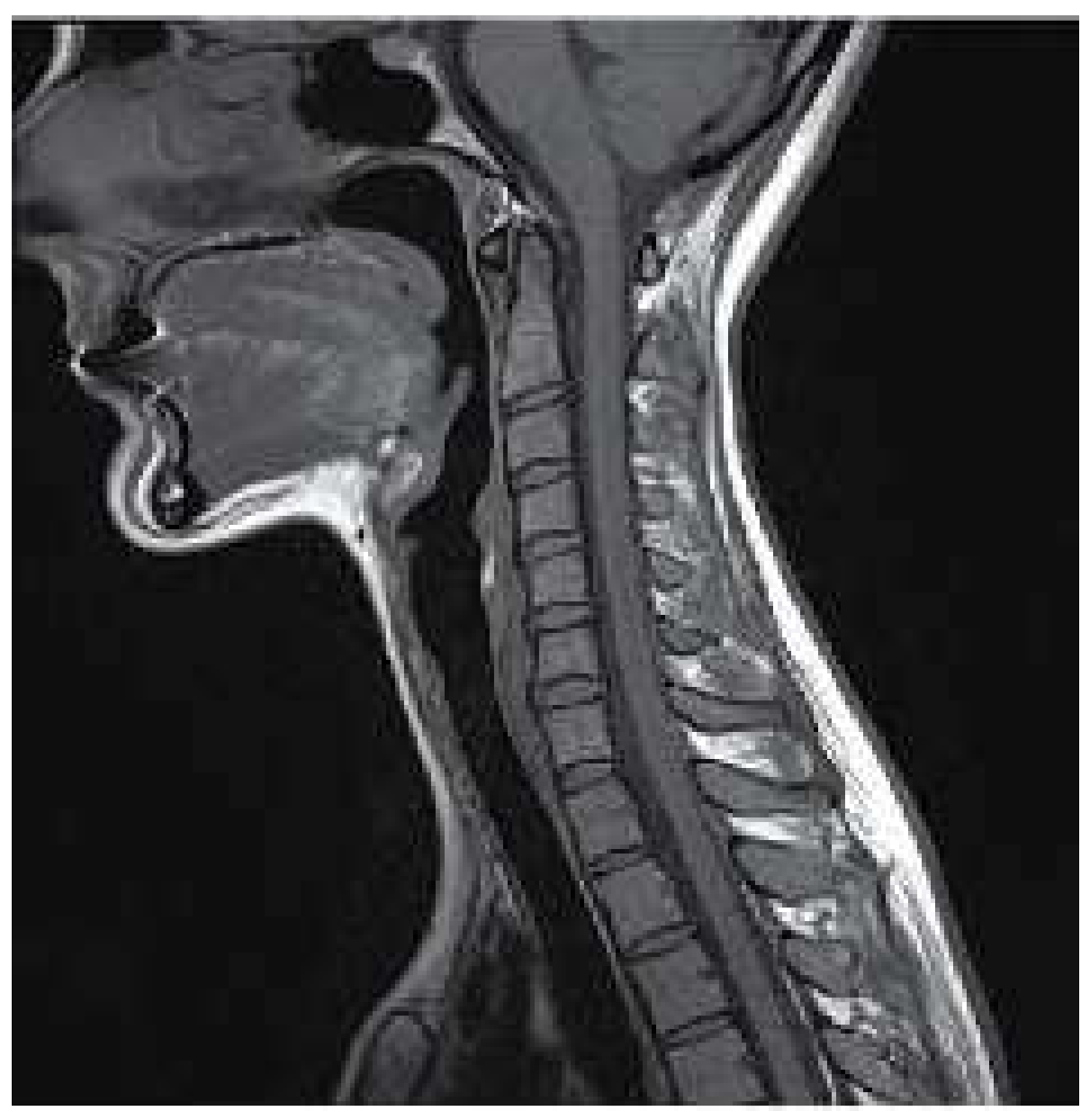
MRI is a non-invasive technique widely used in medicine to obtain medical images needed to make a later diagnosis. This technique is based on the physical phenomenon of resonance; it consist of the transition between different energy states when an atomic nucleus is introduced in an external magnetic field of a characteristic frequency. This frequency, known as Larmor frequency, corresponds to the precession frequency of the protons inside the nucleus. When a magnetic field is applied, the protons absorb the energy and promote to a higher level. Once the magnetic field is removed, the protons decay to the ground state. MRI measures the time and energy released from this last transition. Because of their surroundings, those two values will be different for each proton. Then, by applying the Inverse Fourier Transform to the obtained data it is created the image with different contrast for each component of the body [
12], as shown in
Figure 1.
This technique allows to distinguish different components of the human body, in particular soft tissues as muscles, tendons, ligaments, fats, etc. Not only that, it also makes it possible to differentiate between bones and organs [
12]. The images can be in any direction or part and they can even be made of animals, for instance a mice [
14]. Moreover, MRI can be used as an spectroscopy technique in biochemistry: it allows to know the three-dimensional and dynamic structure of biological molecules [
15]. Additionally, its main advantage over other techniques, such as computed tomography or X-rays, is its lack of ionizing radiation, which makes MRI exams secure for the patient. Because of these reasons, its multiple uses and its high resolution imaging, MRI is known as the jewel in the crown in medical imaging [
16].
Despite the many advantages mentioned before, MRI has some drawbacks: patients with pacemaker or with metal prostheses can be hurt by the strong magnetic field (up to 3T), so they can not be examined. Also, because of the reduced space and the high level of noise in the machine, it can generate stress or anxiety. In addition to these disadvantages, there are many more safety precautions that must be taken in consideration in order to perform an examination. In addition, maintenance of machine components and tests are very expensive. Finally, it takes a lot of time to acquire the data necessary to construct the image, approx. 40 minutes [
17].
In this article we present a methodology to reduce the acquisition time of MRI by using three different CS algorithms. We consider different images of MRI of the head and reconstruct them with less measurements and, therefore, the acquisition time is reduced. In the algorithms, we introduced a number of data smaller than the real image and measure the time the algorithm takes on the reconstruction and the error committed. This study paves then the way for shorter exams in MRI.
The article is organized as follows: in
Section 2 we describe the CS algorithms employed to reconstruct the image and how they can be applied in MRI. In
Section 3, we present and discuss the results (reconstructed images, acquisition time and error). We finish with the conclusions.
2. Materials and Methods
MRI receives the data of proton relaxation and stores it in the frequency space, so that with the Inverse Fourier Transform it is possible to construct the image. The CS problem applied to this case can be written as:
where
y are the frequency samples collected by the machine,
F is the Fourier measurement matrix
x is the image to be constructed and
is the noise randomly distributed. We have to solve an inverse linear problem to recover the data that forms the image from the measurements; we use the measurement matrix which associates a frequency to a value in the grey scale. The object
x can be an image in 2D or 3D but it is represented as a vector by concatenation.
In the ideal case in which enough measurements are taken (
), Eq. (
8) can be solved by applying the Inverse Fourier Transform on the frequencies:
To reduce the acquisition time, less measurements are taken. Therefore, Eq. (
8) has infinite solutions which can be solved with minimization algorithms. In this article, to reconstruct the image we use five possible methods: Iterative Re-weighted Least Squares (IRLS), Iterative Soft Threshold (ISTA), Iterative Hard Threshold (IHTA), a primal dual algorithm (PD) and a log barrier algorithm (LB). The first three algorithms belong to the category of greedy algorithms. They have less accuracy in the reconstruction but is less expensive and simpler. PD and LB are convex algorithms; the error is minor but it takes a lot of computational resources [
7]. All those algorithms shown below, are iterative because of the large storage size of
A.
2.1. Iterative Re-weighted Least Squares
The first algorithm, IRLS, solves the minimization problem without restrictions, Eq.(
7). To achieve this, it replaces the
minimization with
norm with a given weight represented by the diagonal matrix
W In each iteration
k. This matrix is updated by:
where
is the dumping factor which is reduced at each iteration. In order to obtain the reconstructed signal, the algorithm solves Eq.(
11), obtained from the unconstrained lagrangian, until it reaches a certain number of iterations or the solution converges, i.e.
where
is the minimum error [
8].
2.2. Iterative Soft Threshold Algorithm
Next algorithm, ISTA, solves the same minimization problem as the previous algorithm (Eq.(
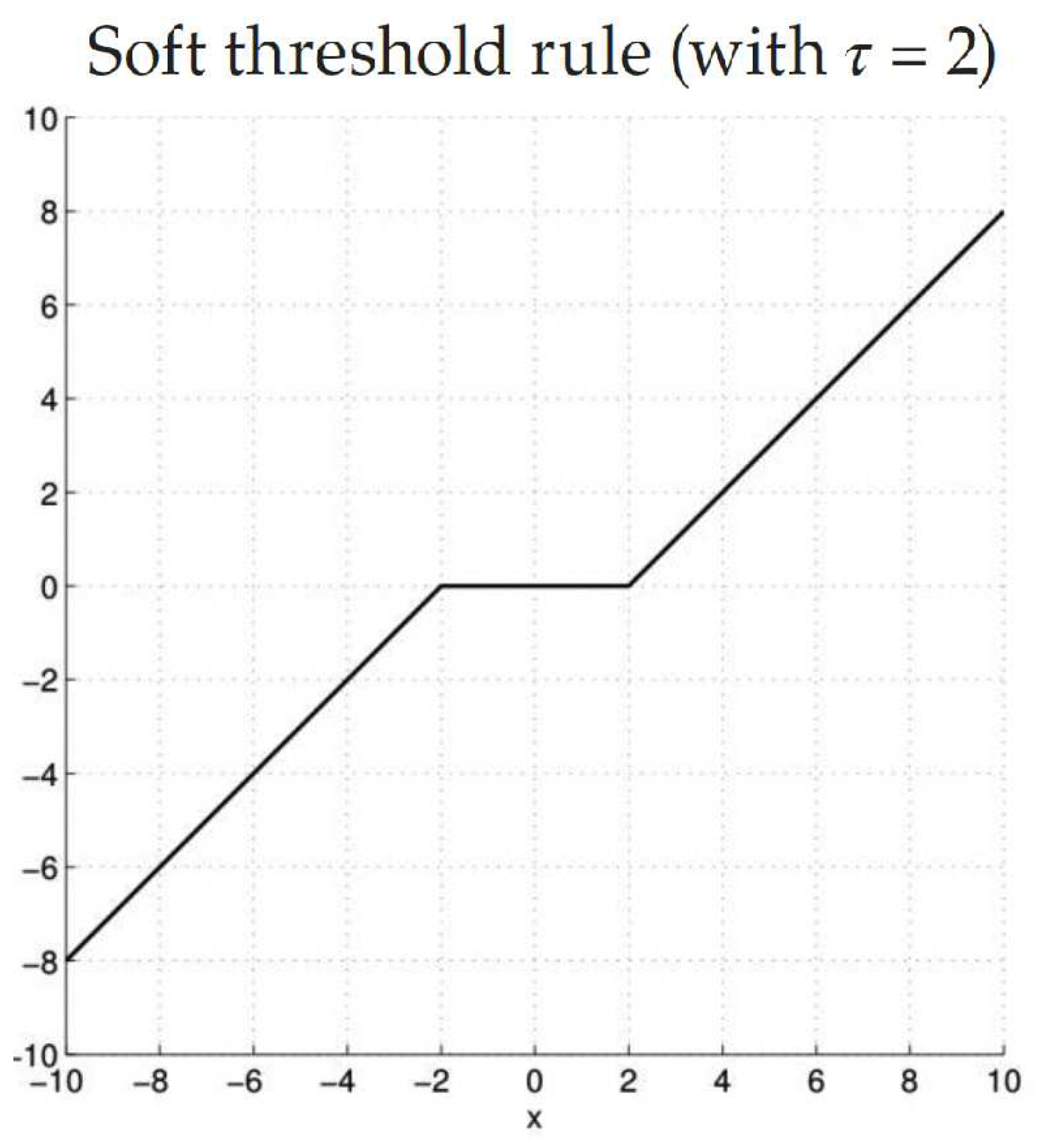
7)). In this case, it is used the function called Soft Threshold:
This, showed in
Figure 2, tries to decrease the amplitude of the coefficients with noise. For example, if the amplitude of the signal is small, the noise and the number of data which provides information are of equal magnitude. The data contains little information and, therefore, the function returns 0. For larger amplitudes, the noise is very small compared to the intensity of the real signal, and thus the function subtracts the part associated with noise [
18].
In order to obtain the reconstructed signal with this algorithm, it is necessary to calculate the Landweber Iteration, which is defined as:
where
a is the largest eigenvalue of the matrix
. The solution
is calculated with the Soft Threshold rule, which is written in a more compacted way:
In each iteration, the value of
should be reduced in order to achieve convergence [
8].
Over the years, ISTA have had a lot of improvements in order to reduce the adquisition time or to get a better resolution. For example, changing the thresholding function to equation Eq.(
15), called p-thresholding function, the technique penalizes small coefficients and shrinks more values to zero. If
, the equation reduces to soft-thresholding (Eq.(
12)) [
19].
Another algorithm which improves the convergence speed, which is ISTA’s main problem, is called fast ISTA (FISTA) which relies on the simplicity of the computation of the proximal map of
norm. If the gradient algorithm is applied in Eq.(
6, it is obtained the following iterative equations:
where
is the stepsize updated in each iteration. Using this idea with the unconstrained problem (Eq.(
7)) it is obtained an iterative scheeme which can be seen as a proximal regularization of
. It is written as:
By using FISTA, the number of iterations required to obtain an optimal solution are less than ISTA as it improves the convergence rate [
20]. However, there is no simple solution to the non-smooth part
. In order to solve this, it is possible to approximate this term by its Moreau envelop, which is smooth [
21]. This strategy is also used in projected ISTA (pISTA) and projected FISTA (pFISTA), in which the unconstrained model is converted into a much simpler form where the objective function can be separated and the orthogonal projection operator is introduced [
22].
It is clear that it has been proposed many ways to optimize MRI and its different sequences that improves its stability, the memory consumption and the reconstruction time [
23,
24], but ISTA is still a good way for signal reconstruction because it stands out for its simplicity.
2.3. Iterative Hard Threshold Algorithm
As mentioned in
Section 1, to solve the CS problem in the
norm is very expensive. However, IHTA handles this problem if the data has noise, i.e.,
In this algorithm, it is defined the following function similar to ISTA:
In this function, if the signal is of the same magnitude as the noise, it eliminates those values; otherwise, it does not alter the value [
8]. In this algorithm the Landweber Iteration is also calculated by Eq.(
13) and the solution is obtained by:
2.4. Primal Dual Algorithm
PD algorithms for linear programming are used to solve equation Eq.(
5) among others. The standard form in linear programs is
where each of the
is a linear functional
for
and
. This algorithm finds the optimal
and the dual vectors
,
, which satisfies the Karush-Kuhn-Tucker conditions, by solving this system of nonlinear equations with the Newton’s Method [
25,
26]:
So in the inner loop of the PD algorithm, Newton’s Method is applied. Conjugate gradients are used in Eq.(
22) in order to obtain the step direction
. Then, update the solution by the next equation:
2.5. Log-Barrier Algorithm
The BPDN problem (Eq.(
6)) can be modeled as Second-Order Cone Programs (SOCPs), i.e., it can be written as a linear program Eq.(
21) where
represents a second-order conic. This method consists of transforming the minimization problem into a series of linear problems in y:
Each one of this subproblems are solved with a high degree of accuracy with the Newton’s method to obtain
. In each iteration
k,
is updated so that
[
26].
2.6. Application of the algorithms to MRI
The previous algorithms have been used to reduce the acquisition time of MRI. Since we were unable to access a MRI machine, we designed a code to read real MRI images, decompose the data and store it as a vector x. This code, also generates the measurement matrix A as a function to avoid memory problems due to the large size of the matrix. The measurements that would be obtained in MRI y are evaluated through A and x. The measurement matrix function calculates the Fourier Transform of x and randomly orders its coefficients. We apply the algorithms to y and obtain the signal and the reconstructed image . Our code also allows to obtain the time it takes to perform the algorithms and the error between the original and the reconstructed signal.
The aim of this article is to reduce the acquisition time and, therefore, the number of measurements taken must be less than the number needed to construct the original image. So, when the image is read, we randomly select a few values which will be stored in x. Then, y is obtained and the signal reconstructed.
We have analysed several images with the algorithms to obtain the parameters of time and error in function of the number of measures. With these results, we select the best algorithm to perform the reconstruction applied to MRI and the minimum number of measures needed to be able to distinguish all image components.
3. Results and discussion
This section presents the results after applying the CS algorithms on medical images obtained with MRI. We analysed several images of the head of the human body obtained from the database of the University of South Carolina [
27].
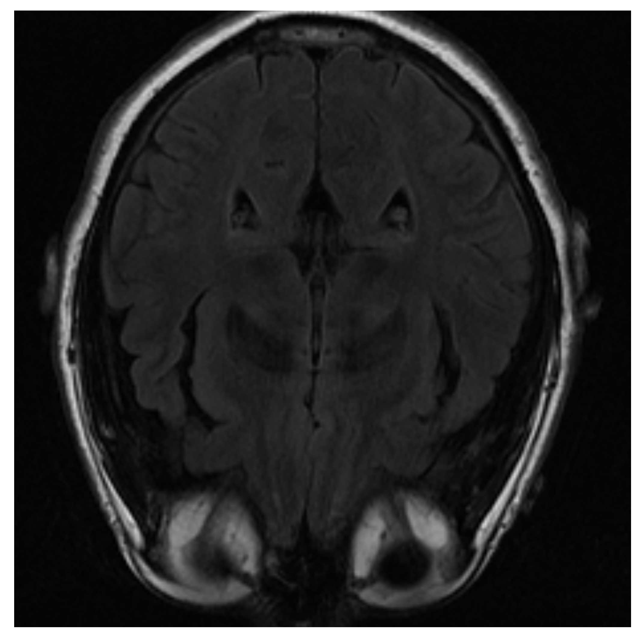
One of the images used in the simulations is shown in
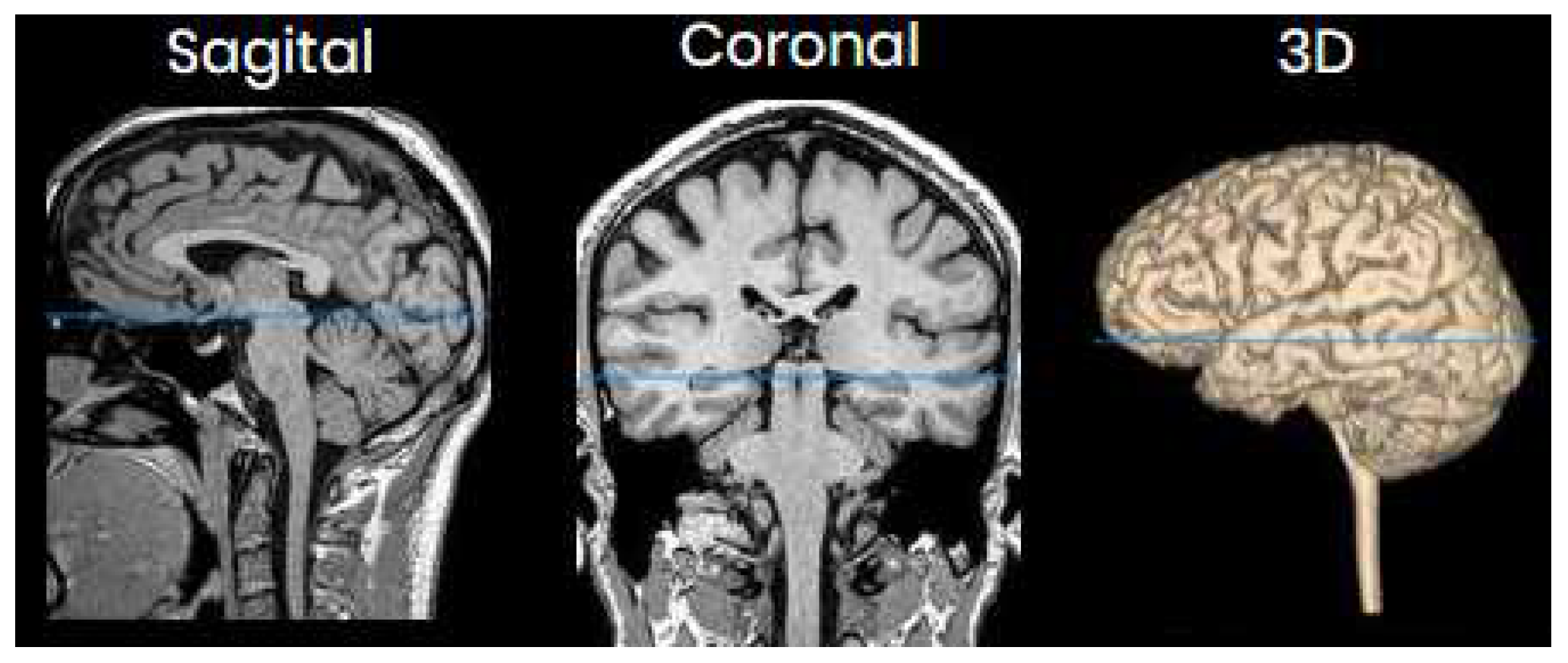
Figure 3 and corresponds to an axial slice of the brain in the plane marked by the blue lines in
Figure 4. In it, the orbit of the eyes can be distinguished at the bottom. Fat appears with a very intense signal, while water and cerebrospinal fluid have a very low intensity.
The image is blurred in the left orbit, which is an example of an artifact. An artifact is a distortion in the image that has no relation to the subject of the region of the studied body. In this case, it has been generated due to the patient’s movement [
28].
Next, we present the images and the parameters obtained from the reconstruction, time and error, for each algorithm as a function of the data taken from the original image.
In the reconstruction by IRLS, only the outline of the head and orbits are detected in the first measurements, while the white matter is not distinguishable (
Figure 5a). When 70% of the data is available (
Figure 5b), the white matter can be distinguished, although it has little intensity. Also, the intensity of the orbits increases and the effect of the artifact starts to be noticed. If the algorithm is run with all the available data (
Figure 5c), the resolution at the edges increases, but the intensity of the white matter signal is lost, which makes its identification more difficult.
As in IRLS, the ISTA algorithm detects first the areas of highest intensity in the first measurements without distinguishing white matter (
Figure 5a). If the number of input data is increased, the resolution of the edges increases but it is still difficult to differentiate the white matter (
Figure 5b). Finally, the resolution increases until the shape of the fat is detected (
Figure 5c).
If it is employed IHTA for the reconstruction, when we use a 30% of the initial signal values (
Figure 7a), much more noise is detected in the inner part of the head, where the white matter should be. In case of a 70% of measurements (
Figure 7b), we obtain an image similar to the same case with ISTA, but the white has more intense signals, which allows to distinguish it better. The resolution increases as more data is added. However, when a 100% of data is reached
Figure 7c), the white matter is not detected, it appears in black.
If we apply PD algorithm the object is much clearer with lower measurements. When it is used 30% of the initial values
Figure 8a), the structure inside the head can be recognized and delimited, even though its low intensity. As the number of measurements is increased, the images get better resolution so when we have 70%
Figure 8b), the image is similar to the original one. Finally, with 100%
Figure 8c), the grey matter loses its intensity.
The images obtained with last algorithm, LB, are more blurred. With 30% of the measurements
Figure 9a) it is not posible to distinguish the structures. It the algorithm works with 70% of the initial data
Figure 9b), the image is reconstructed clearly. In the end, with all 100% of the data, the reconstruction is similar to the one obtained with PD algorithm.
The graph in
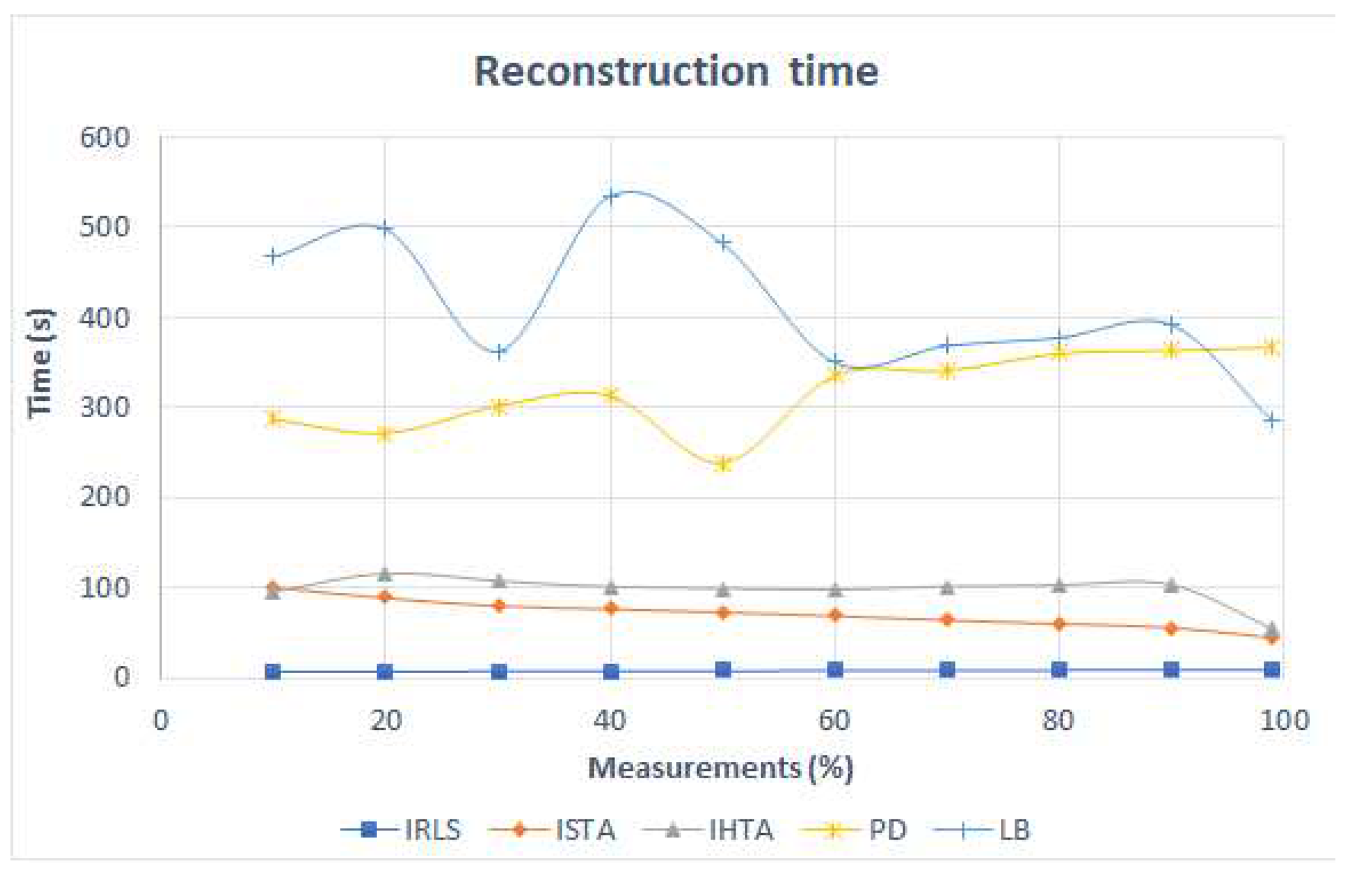
Figure 10 shows the time taken by the algorithms to reconstruct the image as a function of the number of entered data. The IRLS maintains a constant time of 8 s in all reconstructions. It solves the problem of reconstruction in the
norm and it is the fastest one. In case of the ISTA algorithm, which employs a minimization in
norm, the time decreases linearly from 100 s to approximately 50 s. The IHTA algorithm takes the longer time in the reconstructionas it can be predicted since it solves the minimization with
norm. Also, two peaks are obtained at 20% and 90% of the measurements with IHTA. The convex algorithms, PD and LB, takes much more time than the greedy ones as expected. The reconstruction time for PD is higher as the number of measuremets increases. Its maximum value is 367 s. LB algorithm does not show a clear trend. It has three peaks, at 20%, 40% and 90%, the latter being the smoothest one. Finally, with 100% this time decreases to 285 s.
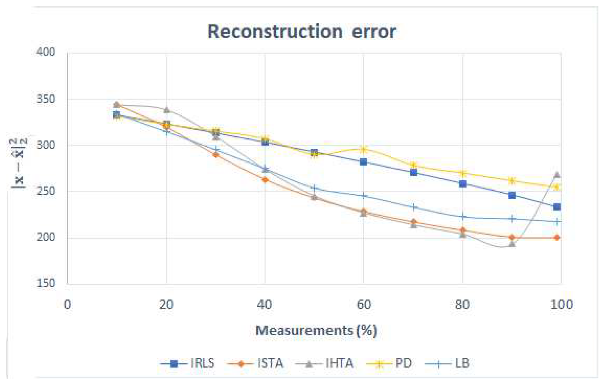
The error made in the reconstruction is found in the following
Figure 11. The IRLS error decreases linearly. ISTA and IHTA are very similar: in both the error decreases with the number of measurements, except when 90% of the measurements are reached, where the error with IHTA increases abruptly. This is due to the fact that, as mentioned above, in this last reconstruction it does not detect the signal related to the white matter and, therefore, the error is very high. The error for PD and LB are higher than expected as they are convex algorithms and the images reconstructed were quite similar to the original. Both algorithms decrease the error similarly until 60%, where the error in PD is higher.
4. Conclusions
In this work, we have studied the CS techniques applied to images adquired with MRI. We have developed several programs that allowed us to quickly and clearly reconstruct an image. We started from a random signal with a smaller number of data than those needed to construct the original image in the conventional way. Then, we generated a similar image with a lower resolution. The algorithms chosen to perform this task were IRLS, ISTA, IHTA, PD and LB.
From the analysis of the images reconstructed with these algorithms it can be concluded that it is appropriate to use ISTA. Although it has an adequate computational time and in some cases it may not provide the best possible resolution, it allows to distinguish each component if 70% or more of the measurements are taken. Although the IHTA algorihtm has the highest resolution, it does not solve some images correctly and takes more time perform the reconstruction. The IRLS algorithm has the shortest computational time, but, like IHTA, it does not achieve enough accuracy. If there are less than 50% of the measurements, it should be used PD algorithm, since its images are clearer and it can recover the structures. LB algorithm takes too much time and does not give any improvement compared to the other algorithms.
These algorithms can be applied to different parts of the human body and with different MRI sequences as , or proton density. These sequences change the contrast of the images, allowing to draw a distinction between components of the human body. The images can also be reconstructed even if contrast agents were introduced.
The same CS technique studied in this article can be applied to other methods; for example, computed tomography or X-ray. Although the acquisition time of these is much shorter, it can still reduce the amount of radiation applied to the human body needed to obtain an image.
