1. Introduction
Recently, with the increasing improvement of material life and cultural demands, people pay more and more attention to the pursuit of a favorable light environment. Light pollution has generated huge costs, reaching nearly
$7 billion annually in the United States [
1]. According to Gaston et al. [
2] , over one-tenth of the land area on Earth is illuminated by artificial light at night. Furthermore, if skylight is included, this proportion will increase to 23%. To assess the risk level of light pollution in the economic system, it is necessary to establish a widely applicable measurement standard. However, nowadays, the overall causal system of light pollution remains incomplete. There are gaps in the evaluation system and pollution mechanisms of light pollution.
Light pollution refers to unnecessary, inappropriate, or excessive artificial lighting [
1]. Regarding the composition of light pollution, light pollution is generally divided into white light pollution, daytime pollution, and color pollution. With the attention paid to the problem of light pollution, more and more scholars have conducted research on the causes of light pollution. The cause of light pollution is not only attributed to one factor but the result of a complex interaction of many factors, including transportation [
3], mineral resources [
3], topography [
3], and income [
4,
5]. All of them contribute to varying degrees of light pollution. Sung et al. [
6] believe that light pollution is affected by residential density at the same height. The above are all studies on the causes of light pollution. At the same time, many scholars have studied the effects of light pollution. When the concept of light pollution was first introduced, governments and scholars focu on its impact on astronomical phenomena [
7]. According to the study by National Geographic, the main effect of light pollution can be divided into three aspects, thus determining the risk level of light pollution in the economic system, social system, and ecosystem, respectively.
Despite some robust strategies adopted by community officials and local groups to try to slow down or eliminate light pollution, the fact remains that light pollution levels are gradually increasing. Its influence is growing. It is supposed that the effects of light pollution are mainly divided into negative effects and positive effects. The negative effects are mainly on animals [
8,
9,
10] and human health [
11,
12,
13]. Owens et al. [
8] explore that artificial light at night would affect the movement, foraging, reproduction, and predation of insects, leading to a decline in the number and total number of local insect species. McLaren et al. [
9] discover that light significantly impacted the choice of stopover sites for migratory birds. Poor-quality stopovers can be detrimental to the conservation of migratory bird species. Thiel et al. [
10] calculate and analyze that a certain degree of light pollution would interrupt the photosynthesis of plants. The effects of light pollution on human health are also multifaceted, such as sleep quality [
13] and the incidence of breast cancer [
11]. Cao et al. [
13] obtain that light pollution would directly interfere with the natural light-dark cycle and destroy the inherent circadian rhythm of organisms, thus seriously affecting the quality of sleep. Walker et al. [
11] find a significant association between ALAN and cancer. The positive effects are mainly concentrated on the decrease in crime rate [
14]. However, there is considerable controversy in the academic circle on this point [
15]. Steinbach et al. [
15] think that light pollution has no positive effect on road accidents or crime in England and Wales.
Chalkias et al. [
16] introduce a light pollution modeling method using geographic information systems (GIS) and remote sensing (RS) techniques in an attempt to address environmental assessment problems in sensitive suburbs. When establishing light pollution indicators, Rabaza et al. [
17] establish a light pollution measurement model based on astronomical methods.
Garstang [
18] creates a map model to observe the changes in skylight at different heights and azimuths from different observation points, effectively quantifying the brightness of artificial light. Gaston et al. [
19] propose species link schemes such as limiting the duration of lighting, changing the intensity of lighting, and changing the spectral composition of lighting to reduce the harm of sunlight and light pollution. Glass curtain wall materials are commonly used in high-rise residential buildings built in cities. Sunshade umbrellas can be divided into two types: vertical sunshade umbrellas and horizontal sunshade umbrellas.
The main points of this paper are summarized as follows:
(1) For the first time, this model is used to study and assess levels of light pollution risk.
(2) By combining the entropy weight method, an appropriate weight coefficient is selected to ensure the accuracy of the Markov random field model.
(3) A intervention strategy is proposed to solve the light pollution problem, and a simulated annealing algorithm is used to determine the best intervention strategy for different positions.
2. Develop a Broadly Applicable Metric
A broadly applicable metric is developed to determine the level of light pollution risk at a specific site. First, the main influencing factors of light pollution, namely indicators, are selected. Then, the data of corresponding indicators in different locations is collected and used to determine the evaluation system of light pollution.
2.1. Index Determination and Data Collection
Xiang et al. [
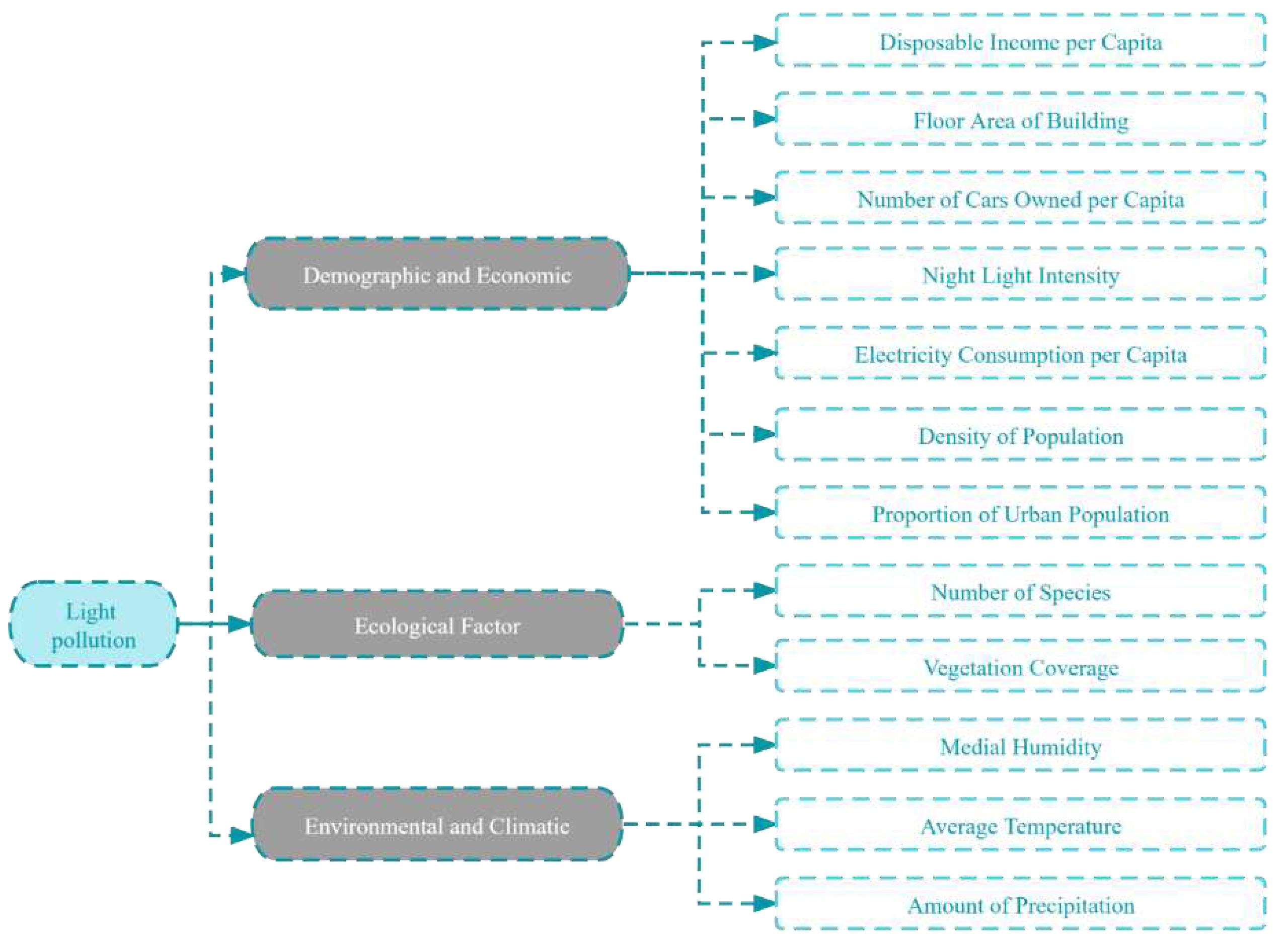
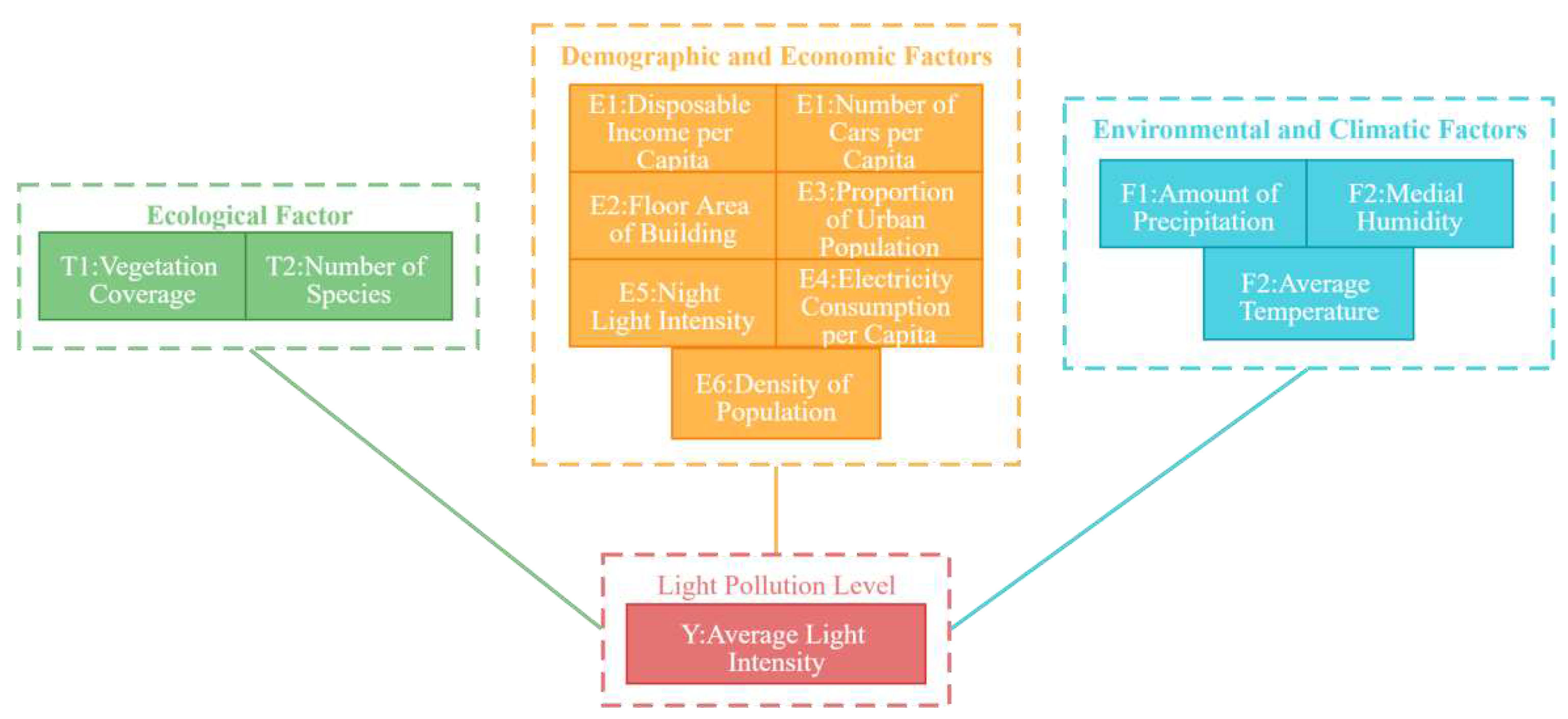
20] use calibrated night-time light images to study spatial-temporal changes in light pollution in China’s PAs from 1992 to 2012 and find that the impact of light pollution can be influenced by various factors, such as the local level of development, population, biodiversity, and geography. To better understand the complex relationship between these factors and the extent of light pollution, it is crucial to establish a comprehensive set of indicators. These factors are identified, analyzed, and distilled into 12 indicators, which have been used to develop a location-based light pollution risk assessment index (LBLPRAI). The index is designed to provide a standardized way of assessing the level of light pollution risk across different locations.
The LBLPRAI is a valuable tool for policymakers and stakeholders to evaluate the severity of light pollution in specific locations and to prioritize appropriate mitigation measures. The 12 indicators include disposable income per capita, floor area of the building, number of cars owned per capita, night light intensity, electricity consumption per capita, the proportion of the urban population, number of species, vegetation coverage, medial humidity, average temperature, and amount of precipitation. These indicators have been carefully selected to represent the different aspects of light pollution and capture each location’s unique cha-characteristics to demonstrate the effectiveness of LBLPRAI and specific data are collected for 12 indicators in five typical Chinese cities, as reported in the 2022 China Statistical Yearbook and the 2022 China Sleep Research Report. By examining the data for each indicator, a better understanding of the relationship between the extent of light pollution and the various factors that contribute to it in different locations can be gained.
Figure 1.
Location-based light pollution risk assessment index.
Figure 1.
Location-based light pollution risk assessment index.
2.2. The Establishment of LBLPRAI
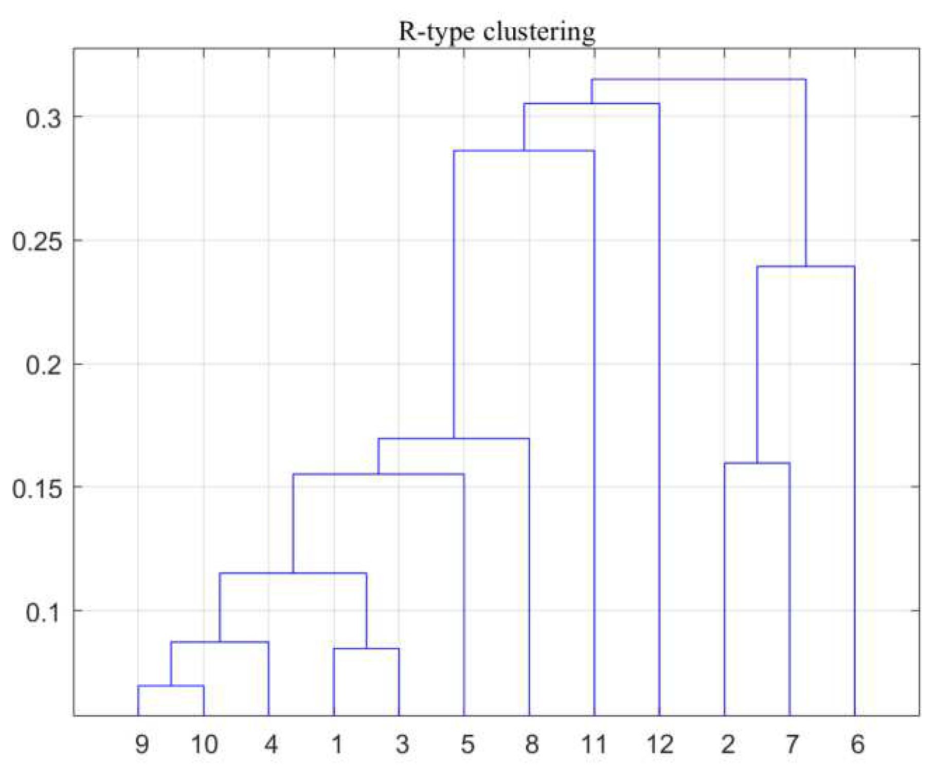
In the process of system analysis or evaluation, to avoid missing some important factors, as many indicators as possible are considered when selecting indicators at the beginning. However, the number of variables is too large, and the degree of correlation between variables is too high, which brings great inconvenience to analysis and modeling. Indicator data are collected from 5 representative cities, and in order to determine the distance between clusters, Euclidean distance and used R-type clustering algorithm are chosen to perform clustering analysis on 12 variables[
21,
22]. The R-type clustering algorithm is used to perform clustering analysis on 12 variables. The results are shown in
Figure 2.
It can be seen from
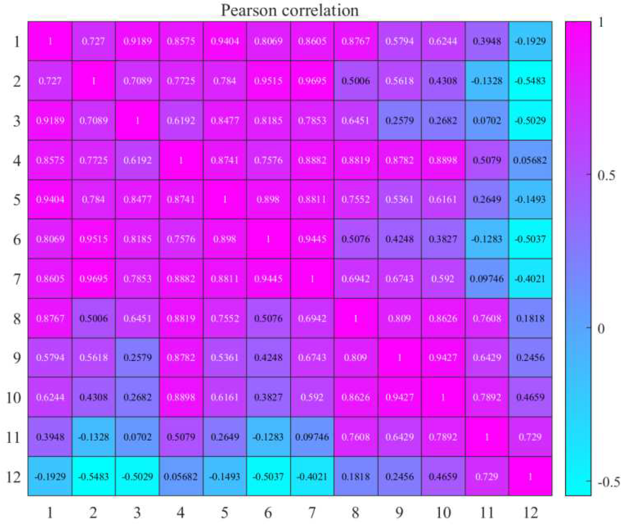
Figure 2 that per capita disposable income is grouped with the number of cars per capita and the average humidity is grouped with moderate temperature. The factor index after clustering is ten items. Through correlation analysis [
23] between different indicators, These two categories have a high degree of correlation, as shown in
Figure 3.
The correlation coefficient between per capita disposable income and the number of cars per capita was 0.92, and the correlation coefficient between average humidity and the average temperature was 0.94. The correlation coefficients of these two categories are high, so the above four indicators are clustered into two.
According to the variation degree of each index, information entropy is used to calculate the entropy weight of each index to obtain a relatively objective index weight. Before this, partial negative data need to be processed to make all indicators positively correlated with light pollution.
indicates raw data,
indicates the processed data.
After standardizing the data, the entropy weight method is established [
24,
25]to analyze the weight. There are
evaluation objects,
indicator variables, and the value of the
th evaluation object regarding the
th indicator variable is
for
, construct the data matrix
. Calculate the proportion of the
th evaluation object with respect to the
th index variable
Calculate the entropy value and coefficient of variation of the
th index variable
So the weight of the
th index variable is gotten
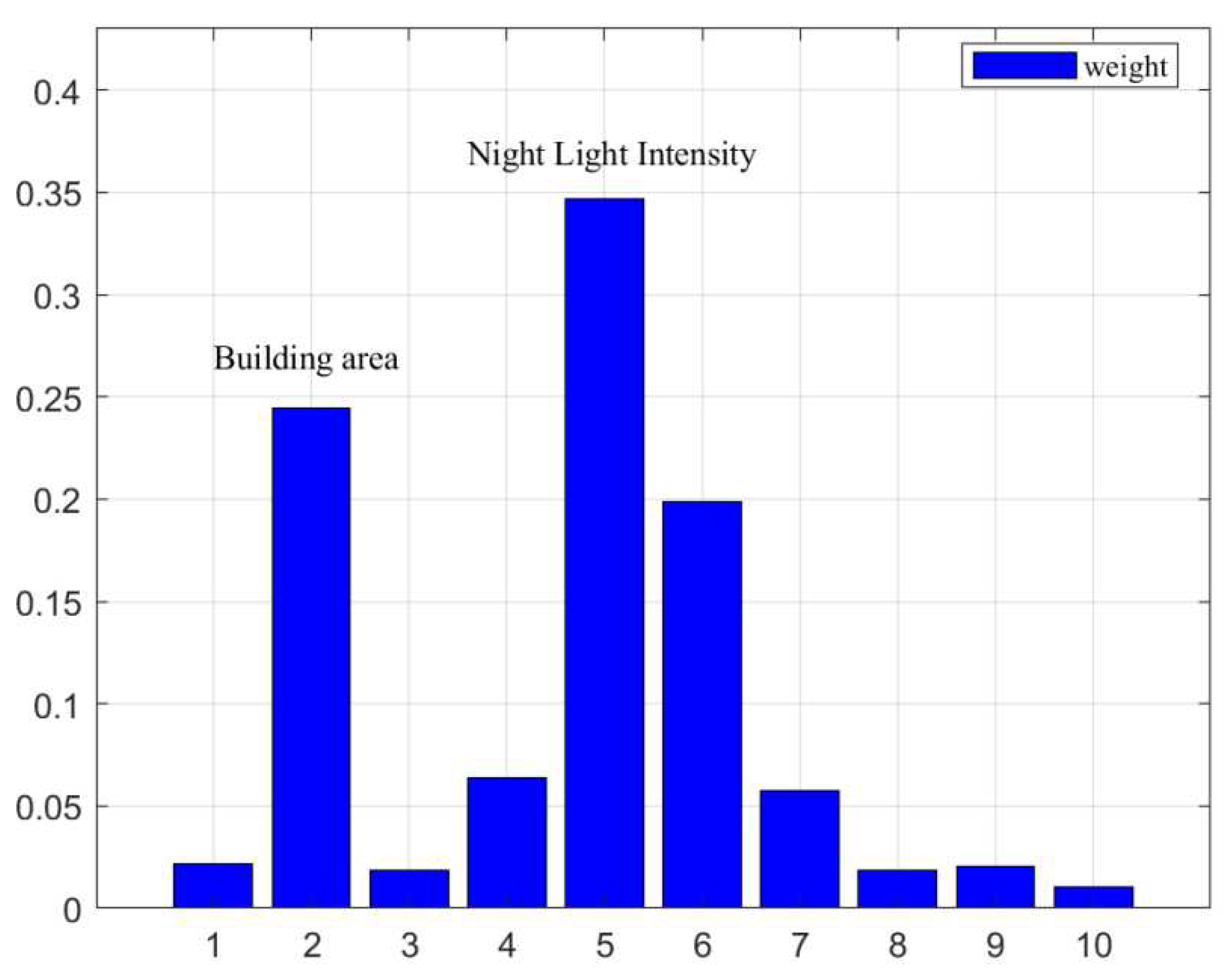
According to the data collected above, the weight of each indicator obtained is shown in
Figure 4. It is found that the weight of building area and highway lighting brightness is the largest, reaching 0.24 and 0.35, respectively, indicating that these two indexes have a more significant impact on the dedication level of light pollution.
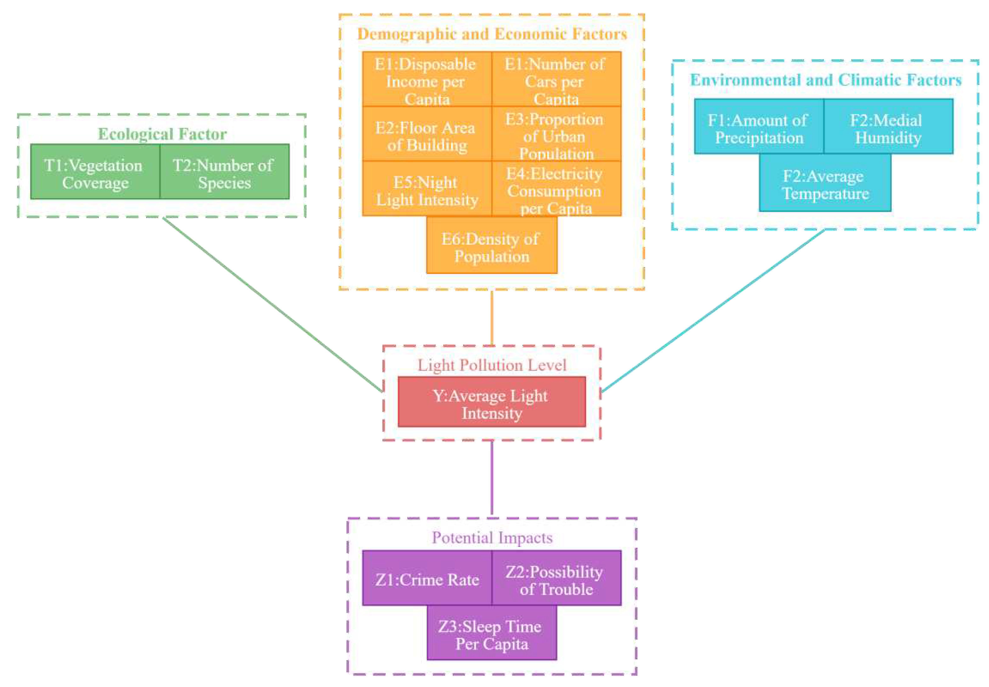
To develop a broadly applicable metric for measuring the level of light pollution risk, the clustering results and the indicator classes are used first to which different indicators belong. The ten indicators are classified into three impact indicators: demographic and economic factors, environmental and climatic factors, and ecological factors, denoted as
,
, and
, respectively. It is believed that average light intensity can represent the risk level of light pollution, and all three indexes can affect the risk level of light pollution. The relationship between these indicators can be represented by the undirected probability graph, as shown in
Figure 5. The boxes indicate indicators, and the lines indicate that they are correlated but not wholly causal. The posterior probability of risk index is modeled as exponential family distribution, which can better deal with the complex relationship between different indicators. By modeling these indicators as Markov random fields [
26,
27], their interactions can be better understood and provide more scientific methods and tools for risk assessment and control.
Conditional probability can be decomposed into the product of multiple exponential distributions as follows:
where
represents the random variable average light intensity,
represents the exponential distribution, and
is a constant so that the value range of the right formula is
.
Considering the different weights of different indicators in the index class
, multiply the indicators with the corresponding weights and increase the activation function [
28]
thus (5) is equal to
where the activation function is
Next, the
in the above formula is determined by using the maximum likelihood method.
Using the collected data and taking the minimum loss function as the objective, the parameter
can be obtained:
The parameters are determined for
and believe that the is the th LBLPRAI region.
3. LBLPRAI Applied to Four Diverse Types of Locations
Different locations are categorized into four types:
Protected land: Areas that are protected by government or private entities from development for their ecological, cultural, and natural importance;
Rural community: A community located in one of the sparsely populated areas of a country or region, which is not easily accessible from urban communities;
Suburban communities: located in areas with moderate population density in a country or region or easily accessible from urban communities;
Urban community: A community located in one of a country or region’s most densely populated areas.
The light pollution risk levels of four different types of sites are obtained by collecting the data from four different types of locations and bringing the model established before into the accurate data calculation. The reasons for the results are analyzed below.
3.1. LBLPRAI of Four Diverse Types of Locations
The data is collected from five different areas, including one protected land, one rural community, one suburban community, and two urban communities. LBLPRAI analysis is conducted in this paper on them respectively and obtained the results as shown in
Table 1.
LBLPRAI is used to measure the degree of light pollution. Namely, an increase in LBLPRAI corresponds to a greater severity of light pollution. According to the results in
Table 1, light pollution in protected land is the least, followed by that in rural communities, suburban communities, and urban communities.
3.2. Analysis and Evaluation of Results on Four Diverse Types of Locations
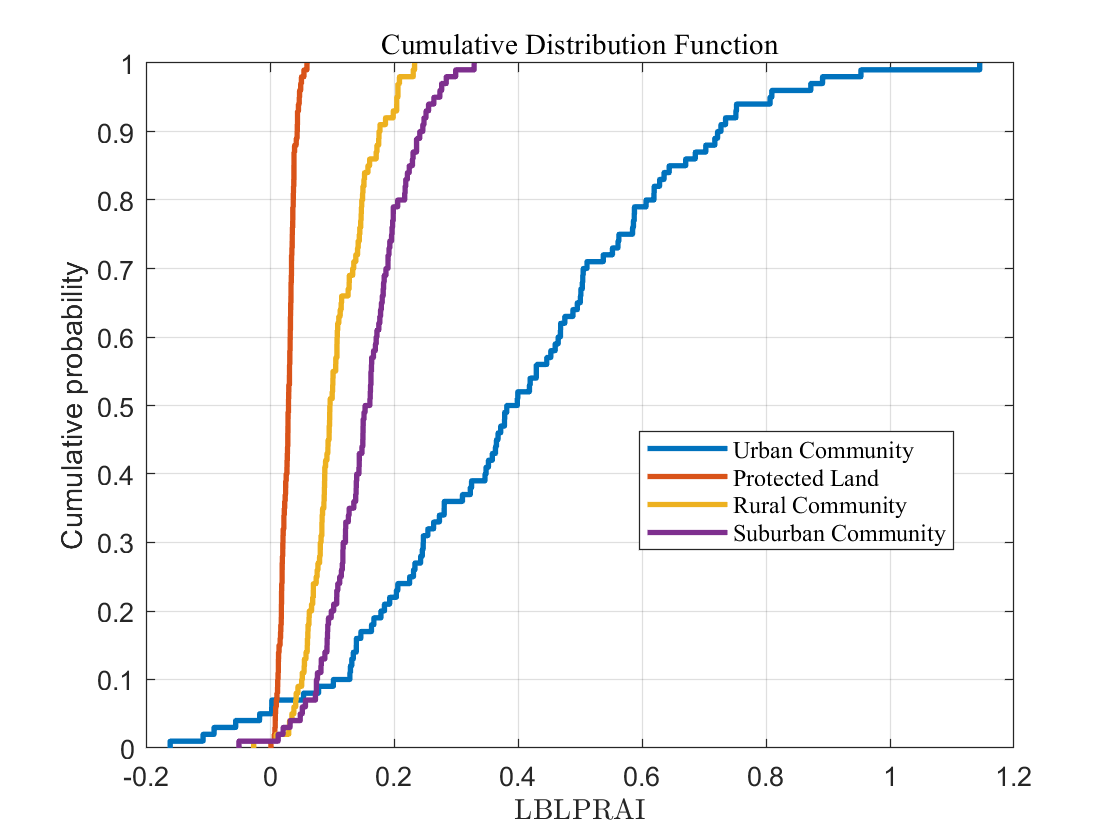
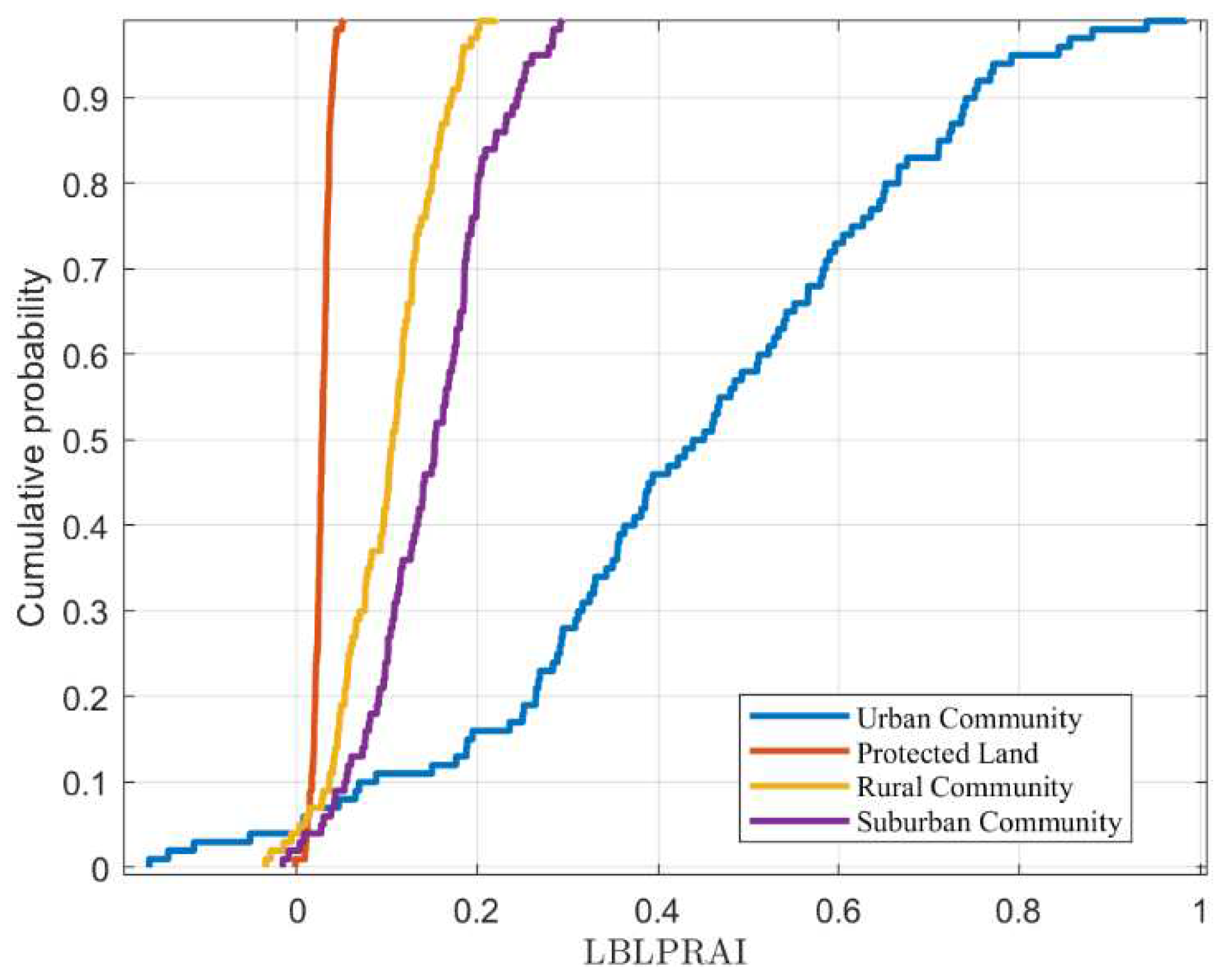
In order to visually see the influence and relationship of four different types of areas on the risk level of light pollution under the indicators selected. It is assumed that the data of an indicator is usually distributed in the same type of region. One hundred values are taken that fit the normal distribution, so 100 sets of 10-dimensional data are gotten in the same type of location. Eq. (2) is used to calculate the LBLPRAI of each data collection and calculate its cumulative distribution probability.
Plot the cumulative distribution function for different regions, as shown in
Figure 6.
It can be seen from
Figure 6 that LBLPRAI values in urban communities are more extensive and distributed in a broader range, and LBLPRAI values in Protected Land are primarily distributed in the range
. This result indicates that the selected index can distinguish the region type of the data by its influence on the LBLPRAI value.
The results of the LBLPRAI analysis reveal that light pollution is most severe in urban areas. Firstly, urban areas have a higher concentration of artificial light sources, such as streetlights, buildings, and billboards, which emit light upwards and outwards. This creates a significant amount of light scatter and light trespass, leading to a higher LBLPRAI value. In contrast, rural and protected areas have fewer artificial light sources, and their lighting tends to be more directional, reducing the amount of light scatter and trespass. Secondly, urban areas have a higher population density and energy consumption, leading to a higher demand for outdoor lighting. This results in an increase in the number of artificial light sources and longer lighting hours, contributing to a higher LBLPRAI value.
By comparison, light pollution in rural areas is much lower, as the lower population density and fewer buildings result in fewer lighting facilities and, correspondingly, less light pollution. Additionally, rural areas mainly use traditional yellow street lights, which have a smaller range and intensity of light, resulting in relatively lower light pollution.
Suburban areas have relatively less light pollution, but with the acceleration of urbanization, many suburban areas face light pollution problems. Compared to urban areas, suburban areas have lower building and population densities, resulting in lower lighting density. However, due to their proximity to urban areas, they are also exposed to urban light pollution, exacerbating the light pollution problem.
Protected areas have the least light pollution, as human-made light pollution activities are usually not allowed, and the number and intensity of lighting facilities are strictly limited. In addition, the building and population density in protected areas are very low, and there are no commercial facilities or vehicle-generated light pollution, resulting in the least amount of light pollution in protected areas.
LBLPRAI provides valuable analysis and evaluation that helps us better understand the problem of light pollution and provides insights for developing more effective measures to control light pollution.
4. Three Possible Intervention Strategies to Address Light Pollution
Here, three possible intervention strategies are proposed to address light pollution. Some specific actions for each strategy are also provided, and the potential impact of these actions on the overall light pollution level. Furthermore, the relationship between potential impacts and indicators is established.
Figure 7.
The relationship between potential impact and indicators.
Figure 7.
The relationship between potential impact and indicators.
4.1. Three possible intervention strategies
Based on the previous results and models, this paper proposes three possible intervention strategies to address light pollution, which can effectively mitigate the negative impacts of light pollution on humans and the ecosystem or promote positive impacts.
(1) Roadway lighting systems planning
This measure leads to changes in the indicator “Night Light Intensity” directly.
means the “Night Light Intensity” before implementation of the intervention strategy,
represents the “Night Light Intensity” after implementation of the intervention strategy, and
represents the implementation intensity of the intervention strategy
Specific actions are:
Light intensity is one of the primary sources of light pollution, especially in night-time lighting. Some cities set public places, such as roads, too bright for safety and aesthetic purposes, which exacerbates light pollution. Therefore, it is suggested that local governments should plan the lighting system for roads and public places reasonably. They should try to turn on the lights as late as possible when the natural light source is relatively weak and turn them off immediately when it is late at night or when there are few pedestrians. Scientific measurement of the reasonable distance between streetlights should also be considered, considering the brightness and height of the lighting equipment and avoiding setting them too close together to reduce unnecessary waste and aggravation of light pollution. Increasing research and development and upgrading of energy-saving lighting equipment, such as replacing old incandescent bulbs with energy-saving LED lights, can also reduce energy waste and the level of light pollution.
(2) Increasing vegetation coverage
This measure leads to changes in the indicator “Vegetation Coverage” directly.
means the “Vegetation Coverage” before implementation of the intervention strategy,
represents the “Vegetation Coverage” after implementation of the intervention strategy, and
represents the implementation intensity of the intervention strategy
Specific actions are:
Light pollution is harmful not only to humans but also to plants and animals. Increasing vegetation coverage can absorb and mitigate the effects of light pollution, thereby reducing the intensity of light pollution. Social groups, particularly environmental organizations, can enhance people’s awareness of protecting wildlife through lectures, community outreach, and advocacy for residents to participate in tree-planting activities during holidays like Arbor Day. Government officials can also implement related measures, such as earning points for planting a tree or having the naming rights to a tree. The government can also increase the development of barren land to increase vegetation coverage and reduce the intensity of light pollution. Social groups and the government should work together to enhance people’s awareness of increasing vegetation coverage and encourage more people to participate. In addition, the construction of green belts along roads or around cities planting trees, shrubs, and other vegetation can effectively increase the area covered by vegetation.
(3) Building system planning
This measure leads to changes in the indicator “Floor Area of Building” directly.
means the “Vegetation Coverage” before implementation of the intervention strategy,
represents the “Vegetation Coverage” after implementation of the intervention strategy, and
represents the implementation intensity of the intervention strategy
Specific actions are:
When the building density of a city increases, the level of light pollution in the city also tends to increase. One of the primary sources of light pollution is outdoor lighting, and high-rise buildings are one of the most common lighting sources. The higher the building, the more comprehensive the range of light pollution it produces. In particular, the number of high-rise buildings is often very dense in the city center, making the problem of light pollution in the city center particularly prominent. Therefore, reducing building density can be an effective way to address light pollution.
Firstly, urban planning authorities should consider the problem of light pollution in the urban design process to ensure that as building density increases, it does not cause more significant pollution to the surrounding environment. Secondly, urban planning departments can construct more residential areas on the city’s outskirts to accommodate the growing population while reducing the population density in the city center. In this way, high-rise buildings can be distributed more evenly in various city areas, thus reducing light pollution.
In addition, urban planning departments can encourage developers to adopt the concept of “green buildings” by selecting more environmentally-friendly building materials and designs to reduce the impact of buildings on the environment, including reducing the impact of light pollution. The exterior lighting systems of buildings should be planned and designed rationally, using energy-saving and low-light-polluting lamps to avoid over-illumination and reflection. For those buildings that still require lighting at night, such as hospitals and public places, the exterior lighting system of the building should only be turned on when necessary or use shading measures to reduce light pollution.
4.2. Potential Impacts
Firstly, potential impact indicators are selected to examine the effectiveness of the three proposed measures and explore their potential impacts. Since some communities that choose to implement low-light policies may experience an increase in crime rates, we can select the possible impact indicator of crime rate and denote it as . Similarly, reducing the use of lighting may lead to an increase in traffic accident frequency, so we select the potential impact indicator of accident rate and denote it as . Light pollution also has an impact on wildlife and plants, so we select the potential impact indicator of “Sleep Time Per Capita” and denote it as .
Different strategies will not only lead to changes in the risk level of light pollution but also affect potential indicators. The focus of partial least squares regression (RLS) research [
29,
30] developed in recent years is that multiple dependent variables can model multiple dependent variables regression, which can model under the condition that multicollinearity exists between independent variables and has a solid ability to explain dependent variables. Partial least squares regression analysis is used to establish the relationship between different indicator variables and three potential impact indicators.
Let represent the indicator variables, and represent the potential impact indicators. We have evaluation objects, indicator variables, and potential impact indicators. After data standardization, the data matrices and is constructed.
The first pair of components from two variable sets are extracted while maximizing their correlation.
Suppose the regression model is
where
and
say in the residual error matrix,
,
for the parameter vector in the regression model, using the least squares estimate parameter vector:
Let the rank of
be
, has
component
, so that
Using
to get the partial least squares regression equation of
potential influence indexes:
where
,
.
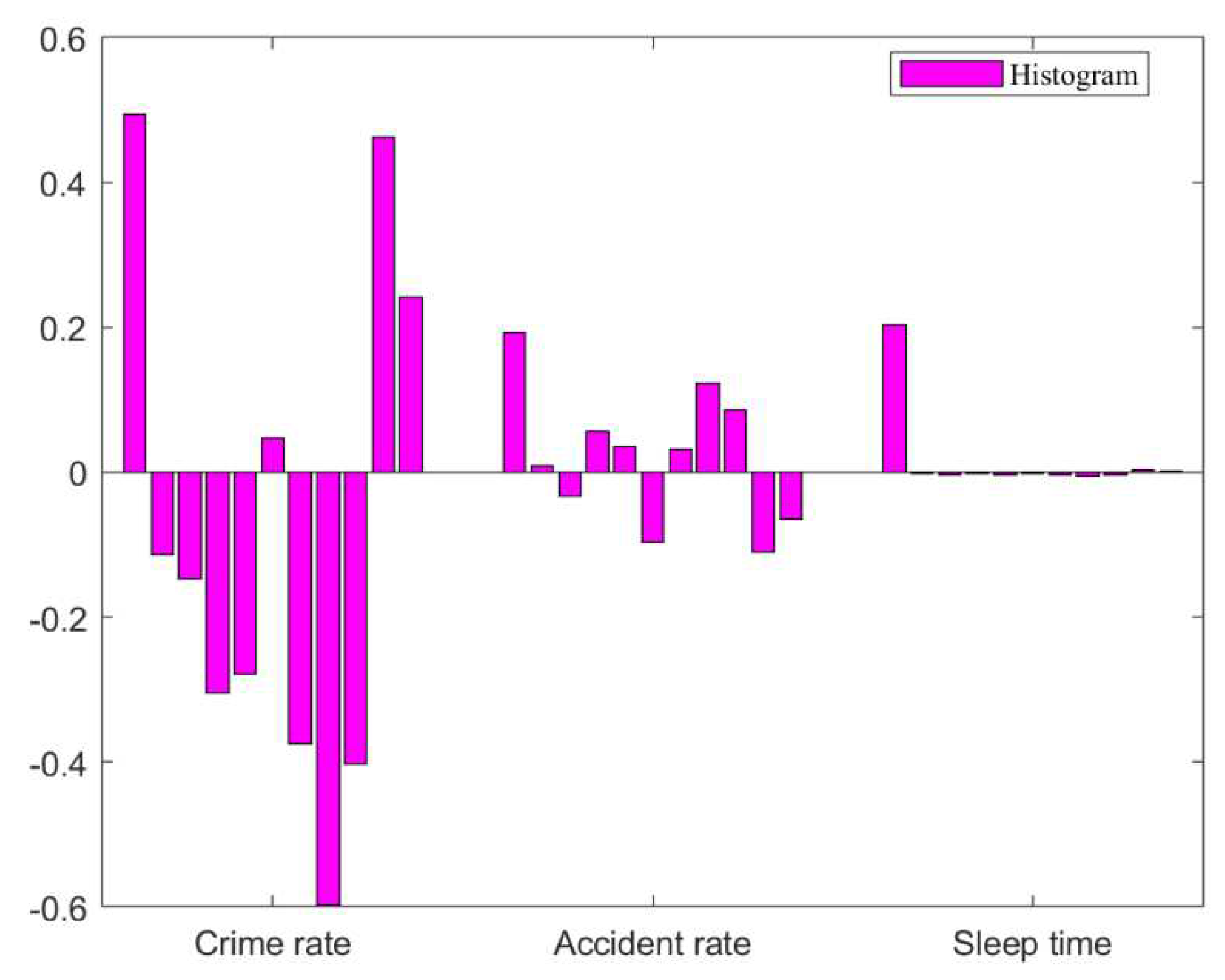
The collected data is used in the model to observe each independent variable in the interpretation of , and the regression coefficients of each coefficient are plotted as follows:
Figure 8.
Regression coefficient diagram.
Figure 8.
Regression coefficient diagram.
It can be seen from
Figure 9 that disposable income per capita has a significant impact on the three potential variables, and the increase in night light intensity can reduce the crime rate to a certain extent.
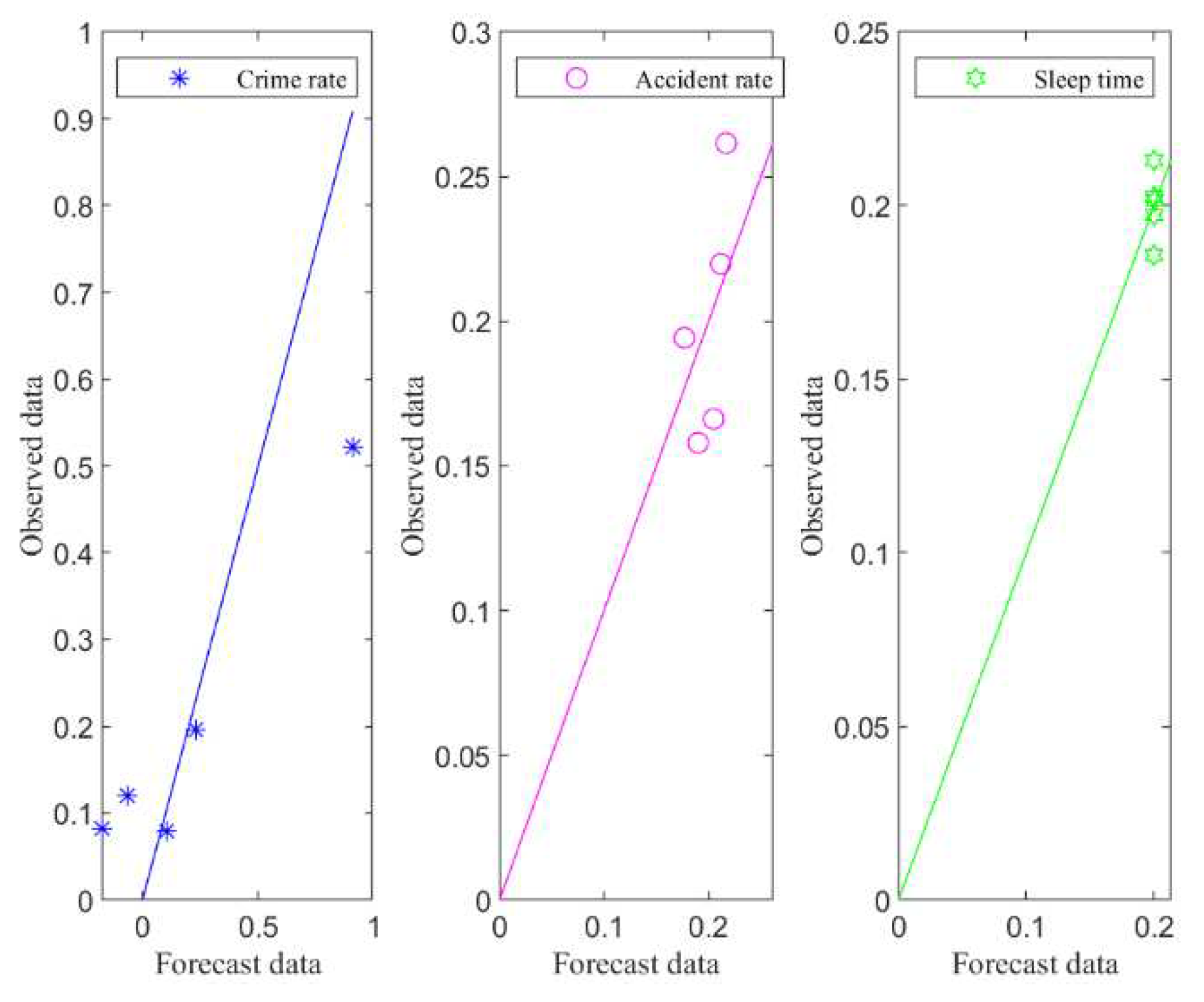
Examining three regression equation model accuracy to is the coordinate value, and the prediction graph is drawn for all sample points:
In this prediction chart, data points are uniformly distributed near the diagonal line, indicating that the fitting effect of the equation is satisfactory.
4.3. Analysis and Evaluation
In order to reflect the impact of intervention strategies on the level of light pollution risk and the three potential impact indicators, the difference between the output value after adopting the intervention strategy and the true value without intervention will be calculated. The change in light pollution risk level is calculated as follows:
The change in light pollution risk levels is
The change in crime rate is
The change in accident rate change is
The change in sleep time is
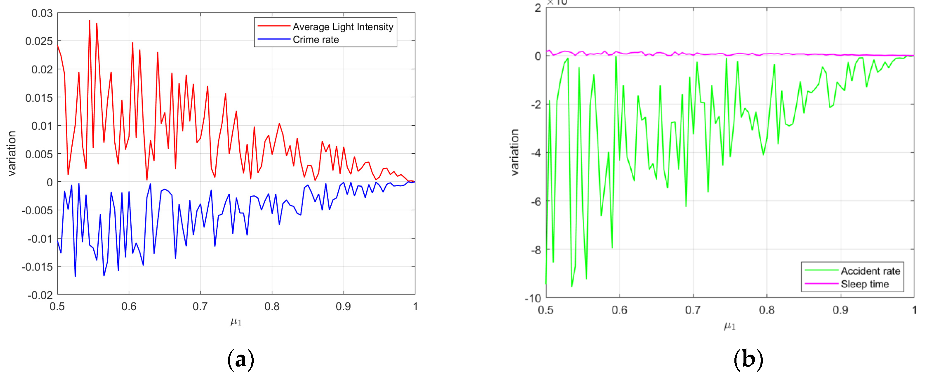
Taking urban community one as an example, if strategy (1) is taken to plan the lighting intensity road lighting system and parameter values are set as the initial value 0.5, end value 1, and step size 0.005, the light pollution risk level and the change amount of three potential influence indicators are obtained along with the curve of parameter .
Figure 10.
(a) Intervention strategy (1) Impact on light pollution level and crime rate; (b) Intervention strategy (1) impact on accident rate and sleep time.
Figure 10.
(a) Intervention strategy (1) Impact on light pollution level and crime rate; (b) Intervention strategy (1) impact on accident rate and sleep time.
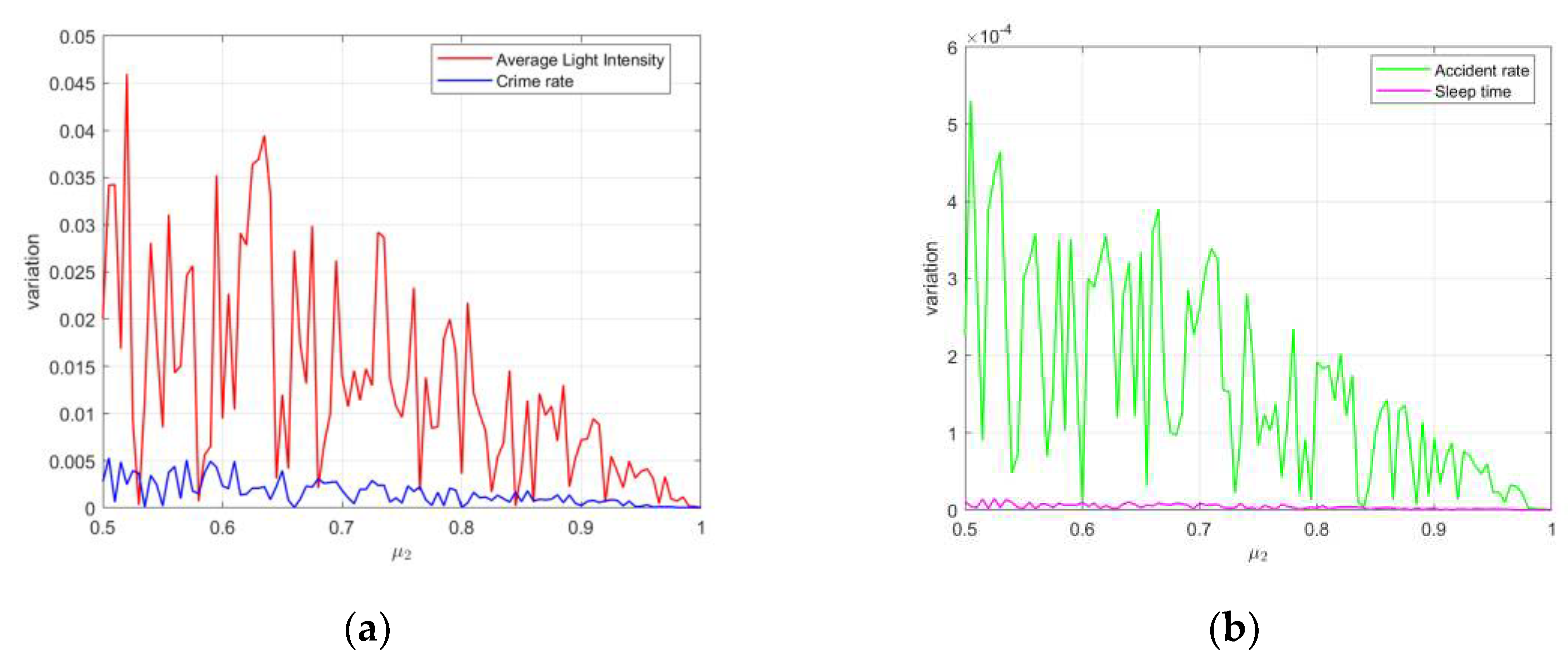
If intervention strategy (2) is taken to increase vegetation coverage, with the initial parameter value set to 0.5, the end value to 1, and the step size to 0.005, we can obtain the curves of the changes in light pollution risk level and the three potential impact indicators with respect to the parameter .
Figure 11.
(a) Intervention strategy (2) Impact on light pollution level and crime rate; (b) Intervention strategy (2) impact on accident rate and sleep time.
Figure 11.
(a) Intervention strategy (2) Impact on light pollution level and crime rate; (b) Intervention strategy (2) impact on accident rate and sleep time.
Taking intervention strategy (2) can lead to a significant reduction in light pollution risk level, but its impact on the three potential impact indicators is minimal.
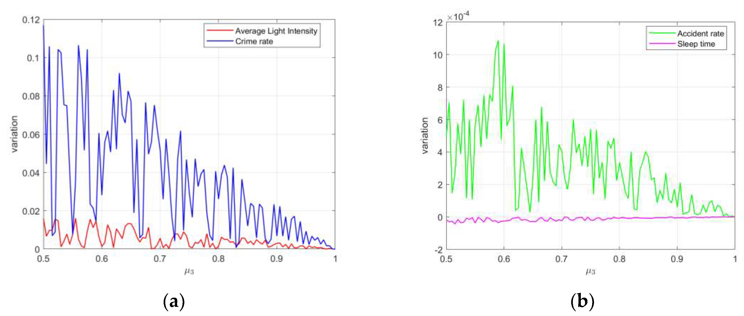
If intervention strategy (3) is taken, with the initial parameter value of 0.5, ending value of 1, and step size of 0.005, the change in light pollution risk level and the three potential impact indicator variables are plotted against the parameter .
Figure 12.
(a) Intervention strategy (3) Impact on light pollution level and crime rate; (b) Intervention strategy (3) impact on accident rate and sleep time.
Figure 12.
(a) Intervention strategy (3) Impact on light pollution level and crime rate; (b) Intervention strategy (3) impact on accident rate and sleep time.
Adopting intervention strategy (3) can lead to less mitigation of light pollution risk levels while also significantly reducing the crime rate and decreasing the accident rate. The impact on sleep time is not significant. Therefore, it can be seen that the reduction of building density has an important impact on the light pollution risk level and Crime rate.
5. Effect of Intervention Strategies on LBLPRAI at Two Locations
In order to make the results more comparable, a site with a higher level of urbanization and a site with a lower level of urbanization should be selected for analysis. Therefore, urban community two and rural community were selected as the active sites of intervention strategies, and the optimal intervention strategies were selected.
5.1. Establishment of Influence Model
In order to determine that the three intervention strategies proposed in this paper are effective in each locality, not only the impact of different intervention strategies on light pollution risk levels but also their impact on potential impact indicators need to be considered. Therefore, set the optimization target to
where,
for
are weight coefficients of different influences, which are satisfied
The analytic hierarchy process [
31] is constructed to determine its weight coefficient, and the given judgment matrix is shown in
Table 2.
Using the analytic hierarchy process to determine the weight coefficient of
Different intervention strategies will have other effects on the above indicators. To make the impact as evident as possible, an optimization model is built:
To isolate the impact of a single index, it is sufficient to set for the remaining two terms.
5.2. Influence Model Solving
Rural community and urban community two are selected as the active sites of intervention strategies. Three intervention strategies are used separately for these two sites, and a simulated annealing algorithm [
32,
33] is used to solve Eq. (27). The initial temperature
and temperature attenuation coefficient
were set. The number of iterations is 3000 times, and a total of 6 times of solving.
Table 3.
Solution result.
Table 3.
Solution result.
| Rural Community |
|
|
Urban Community 2 |
|
|
| Intervention Strategy (1) |
0.53 |
0.02 |
Intervention Strategy (1) |
0.82 |
0.25 |
| Intervention Strategy (2) |
0.66 |
0.03 |
Intervention Strategy (2) |
0.54 |
0.04 |
| Intervention Strategy (3) |
0.89 |
0.01 |
Intervention Strategy (3) |
0.74 |
0.11 |
It can be seen from the results that intervention strategy (2) is used in the rural community. Namely, increasing the vegetation coverage rate is the most effective measure. In urban community 2, intervention strategy (1) is used. That is, the planning of the illumination intensity road lighting system is the most effective measure.
Among them, the use of intervention strategy (2) in the rural community can reduce the light pollution risk level by 1.8%, crime rate by 9%, accident rate by 1.1%, and sleep time by 0.52%. In urban community 2, the intervention strategy (1) can reduce the light pollution risk by 17.2%, reduce the crime rate by 4%, increase the accident rate by 1.7%, and reduce the sleep time by 0.37%, which has little impact on sleep.
5.3. Influence Model Improvement
In the actual situation, community officials or local groups will take a variety of measures at the same time. By solving Eq. (27), the difference is that here for are variables solved by simulated annealing.
It can be seen from
Table 4 that the results obtained by the improved model are better than those obtained by using a single intervention strategy, indicating that the use of three intervention strategies at the same time is the most effective method.
6. Conclusions and Future Work
In this study, the author proposes a Markov random field model as a measurement standard to determine the light pollution risk level of the site. The research results can compare and rank the light pollution levels in different regions and provide a scientific basis for the formulation of relevant policies. The work achievements are as follows:
When selecting indicators to assess the severity of light pollution in a specific location, 12 indicators were carefully selected. The combination of an R-type clustering algorithm and correlation analysis is used to screen the indicators, and the ten indicators finally selected can more accurately reflect the characteristics of different regions, covering all aspects of our living environment, more comprehensively assess the light pollution level in different regions, and better understand the relationship between light pollution degree and various factors causing light pollution in different regions.
Different sites are divided into four types for light pollution assessment. The cumulative distribution probability is used to analyze the degree of light pollution of different types of sites and interprets the results, which can intuitively see the impact and relationship of four different types of regions on the risk level of light pollution under the selected indicators.
The author considers that different strategies will not only lead to changes in the risk level of light pollution but also affect potential indicators. Using partial least squares regression to study the multicollinearity relationship between the indicator variables and the three potential impact indicators, it has a strong ability to explain the dependent variables. After putting forward three possible intervention strategies for light pollution, the potential impact of each strategy on the overall impact of light pollution is evaluated using a partial least squares regression model.
Further research may include increasing human activity patterns, many factors that may affect the level of light pollution and optimization of parameters of the Markov random field.
Author Contributions
Conceptualization, Liangkun Fang and Zhangjie Wu; Data curation, Zhangjie Wu; Formal analysis, Liangkun Fang and Zhangjie Wu; Investigation, Zhangjie Wu; Methodology, Liangkun Fang and Zhangjie Wu; Resources, Zhangjie Wu; Software, Liangkun Fang; Validation, Liangkun Fang, Zhangjie Wu and Yuan Tao; Visualization, Liangkun Fang; Writing – original draft, Zhangjie Wu and Yuan Tao; Writing – review & editing, Zhangjie Wu and Jinfeng Gao.
Funding
This work is supported by National Natural Science Foundation of China under Grant (62073296).
Data Availability Statement
Not applicable.
Conflicts of Interest
The authors declare no conflict of interest.
References
- T. Gallaway, R. N. Olsen and D. M. Mitchell, The economics of global light pollution, Ecological Economics 69 (2010), no. 3, 658-665. [CrossRef]
- K. J. Gaston, J. P. Duffy, S. Gaston, J. Bennie and T. W. Davies, Human alteration of natural light cycles: Causes and ecological consequences, Oecologia 176 (2014), no. 4, 917-931. [CrossRef]
- W. L. Xiang and M. H. Tan, Changes in light pollution and the causing factors in china’s protected areas, 1992-2012, Remote Sensing 9 (2017), no. 10.
- Rafindadi, I. M. Muye and R. A. Kaita, The effects of fdi and energy consumption on environmental pollution in predominantly resource-based economies of the gcc, Sustainable Energy Technologies and Assessments 25 (2018), 126-137. [CrossRef]
- B. Wu and H. Wong, Visualization and analysis of light pollution: A case study in hong kong, ISPRS Annals of the Photogrametry, Remote Sensing and Spatial Information Sciences (2012), 171-176. [CrossRef]
- Y. Sung, Examining the effects of vertical outdoor built environment characteristics on indoor light pollution, Building and Environment 210 (2022). [CrossRef]
- K. W. Riegel, Light pollution: Outdoor lighting is a growing threat to astronomy, Science (New York, N.Y.) 179 (1973), no. 4080, 1285-1291.
- A. C. S. Owens, P. Cochard, J. Durrant, B. Farnworth, E. K. Perkin and B. Seymoure, Light pollution is a driver of insect declines, Biological Conservation 241 (2020). [CrossRef]
- J. D. McLaren, J. J. Buler, T. Schreckengost, J. A. Smolinsky, M. Boone, E. E. van Loon, D. K. Dawson and E. L. Walters, Artificial light at night confounds broad-scale habitat use by migrating birds, Ecology Letters 21 (2018), no. 3, 356-364. [CrossRef]
- 1S. Thiel, T. Döhring, M. Köfferlein, A. Kosak, P. Martin and H. K. Seidlitz, A phytotron for plant stress research: How far can artificial lighting compare to natural sunlight?, Journal of plant physiology 148 (1996), no. 3-4, 456-463. [CrossRef]
- W. H. Walker, J. R. Bumgarner, J. C. Walton, J. A. Liu, O. H. Meléndez-Fernández, R. J. Nelson and A. C. DeVries, Light pollution and cancer, International Journal of Molecular Sciences 21 (2020), no. 24, 9360.
- R. B. Clarke, H. Amini, P. James, M. von Euler-Chelpin, J. T. Jorgensen, A. Mehta, T. Cole-Hunter, R. Westendorp, L. H. Mortensen, S. Loft, J. Brandt, O. Hertel, M. Ketzel, C. Backalarz, Z. J. Andersen and Y. H. Lim, Outdoor light at night and breast cancer incidence in the danish nurse cohort, Environmental Research 194 (2021). [CrossRef]
- M. Cao, T. Xu and D. Q. Yin, Understanding light pollution: Recent advances on its health threats and regulations, Journal of Environmental Sciences 127 (2023), 589-602. [CrossRef]
- Y. Q. Xu, C. Fu, E. Kennedy, S. H. Jiang and S. Owusu-Agyemang, The impact of street lights on spatial-temporal patterns of crime in detroit, michigan, Cities 79 (2018), 45-52. [CrossRef]
- R. Steinbach, C. Perkins, L. Tompson, S. Johnson, B. Armstrong, J. Green, C. Grundy, P. Wilkinson and P. Edwards, The effect of reduced street lighting on road casualties and crime in england and wales: Controlled interrupted time series analysis, Journal of Epidemiology and Community Health 69 (2015), no. 11, 1118-1124. [CrossRef]
- C. Chalkias, M. Petrakis, B. Psiloglou and M. Lianou, Modelling of light pollution in suburban areas using remotely sensed imagery and gis, Journal of environmental management 79 (2006), no. 1, 57-63. [CrossRef]
- O. Rabaza, D. Galadi-Enriquez, A. E. Estrella and F. A. Dols, All-sky brightness monitoring of light pollution with astronomical methods, Journal of Environmental Management 91 (2010), no. 6, 1278-1287. [CrossRef]
- R. Garstang, Night sky brightness at observatories and sites, Publications of the Astronomical Society of the Pacific 101 (1989), no. 637, 306.
- K. J. Gaston, T. W. Davies, J. Bennie and J. Hopkins, Review: Reducing the ecological consequences of night-time light pollution: Options and developments, Journal of Applied Ecology 49 (2012), no. 6, 1256-1266. [CrossRef]
- W. Xiang and M. Tan, Changes in light pollution and the causing factors in china’s protected areas, 1992–2012, Remote Sensing 9 (2017), no. 10, 1026.
- C. Fraser and P. Pylyavskyy, Tensor diagrams and cluster combinatorics at punctures, Advances in Mathematics 412 (2023). [CrossRef]
- S. Zhou, Z. Xu and F. Liu, Method for determining the optimal number of clusters based on agglomerative hierarchical clustering, IEEE transactions on neural networks and learning systems 28 (2016), no. 12, 3007-3017.
- Y. Zhou, Q. Zhang, V. P. Singh and M. Xiao, General correlation analysis: A new algorithm and application, Stochastic environmental research and risk assessment 29 (2015), 665-677.
- J. Ye, Multicriteria fuzzy decision-making method using entropy weights-based correlation coefficients of interval-valued intuitionistic fuzzy sets, Applied Mathematical Modelling 34 (2010), no. 12, 3864-3870. [CrossRef]
- J. Deng and M. Pandey, Optimal maximum entropy quantile function for fractional probability weighted moments and its applications in reliability analysis, Applied Mathematical Modelling 114 (2023), 230-251. [CrossRef]
- Q. H. Zhao, X. L. Li, Y. Li and X. M. Zhao, A fuzzy clustering image segmentation algorithm based on hidden markov random field models and voronoi tessellation, Pattern Recognition Letters 85 (2017), 49-55. [CrossRef]
- J. Baz, I. Díaz, S. Montes and R. Pérez-Fernández, Some results on the gaussian markov random field construction problem based on the use of invariant subgraphs, Test 31 (2022), no. 3, 856-874. [CrossRef]
- H. Zhang, W. T. Wang and B. Xiao, Exponential convergence for high-order recurrent neural networks with a class of general activation functions, Applied Mathematical Modelling 35 (2011), no. 1, 123-129. [CrossRef]
- Y. X. Wang and Z. H. Xu, Statistical analysis for contract cheating in chinese universities, Mathematics 9 (2021), no. 14. [CrossRef]
- Y. C. Su, C. Y. Wu, C. H. Yang, B. S. Li, S. H. Moi and Y. D. Lin, Machine learning data imputation and prediction of foraging group size in a kleptoparasitic spider, Mathematics 9 (2021), no. 4. [CrossRef]
- S. Bekesiene, A. V. Vasiliauskas, S. Hoskova-Mayerova and V. Vasiliene-Vasiliauskiene, Comprehensive assessment of distance learning modules by fuzzy ahp-topsis method, Mathematics 9 (2021), no. 4. [CrossRef]
- C. Y. Yu, A. A. Heidari and H. L. Chen, A quantum-behaved simulated annealing algorithm-based moth-flame optimization method, Applied Mathematical Modelling 87 (2020), 1-19. [CrossRef]
- F. He and Q. Ye, A bearing fault diagnosis method based on wavelet packet transform and convolutional neural network optimized by simulated annealing algorithm, Sensors 22 (2022), no. 4, 1410. [CrossRef]
|
Disclaimer/Publisher’s Note: The statements, opinions and data contained in all publications are solely those of the individual author(s) and contributor(s) and not of MDPI and/or the editor(s). MDPI and/or the editor(s) disclaim responsibility for any injury to people or property resulting from any ideas, methods, instructions or products referred to in the content. |
© 2023 by the authors. Licensee MDPI, Basel, Switzerland. This article is an open access article distributed under the terms and conditions of the Creative Commons Attribution (CC BY) license (http://creativecommons.org/licenses/by/4.0/).
