Preprint
Brief Report

Loan Risk Prediction based on Random Forest Model

Altmetrics

Downloads

136

Views

91

Comments

0

A peer-reviewed article of this preprint also exists.

This version is not peer-reviewed

Submitted:

21 June 2023

Posted:

22 June 2023

You are already at the latest version

Alerts
Abstract
As people's consumption habits change, loan plays a crucial role in our modern society. It provides individuals who do not have sufficient money with funds to purchase residential property or start a business. However, for avoiding unpleasant loan defaults, all financial institutions will first assess the borrower's risk index. By predicting the default risk of the borrower to decide whether to lend money. Machine learning algorithms, including random forest, linear regression and so on, have been benefited most of the real-world applications. With the development of machine learning methods, this paper, based on the personal history loan data of an institution studies the loan default risk, and uses the random forest classification model to predict the possibility of loan default. The result showed that the accuracy of this method was 85.62%, which show its application ability of real-world loan prediction and benefits the manager to decide the degree of risk for loan grant.
Keywords: 
Subject: Computer Science and Mathematics  -   Artificial Intelligence and Machine Learning

1. Introduction

As the society has undergone dramatic changes, people’s consumption concept is also undergoing a great change. Loans have become a vital way to help people ease their financial plight. It provides individuals who do not have sufficient money with funds to purchase residential property or start a business, and it provides income for the banks or other financial institutions by collecting interest from the loan. However, a loss may occur if the borrower is not able to create future value from the fund and result in a bankruptcy. A high acceptance rate may cause the financial institutions to wrongly lend the money to clients who are not able to return it in the future, and a low acceptance rate can result in losing potential customers collecting interest from and affecting the financial institutions’ reputation. Thus, it is important for the banks or other financial institutions to estimate the ability of the borrower returning the money by their information and make an accurate decision of the approval of the loan. With the development of artificial intelligence theory [11,12,13,14,15,16,17,18,19,20,21,22,23,24,25], many scholars have made great achievements in credit risk assessment using machine learning algorithms. For example, Zhang et al. proposed a P2P loan default prediction model based on Term Frequency-Inverse Document Frequency (TF-IDF) algorithm of information retrieval, which improved the prediction accuracy by about 6% [1]. Pan et al. constructed a credit risk classification prediction model for small and medium-sized enterprises in supply chain by using SVM algorithm with information gain, and the results showed that the accuracy of this model was 8.97% higher than that of a single SVM model [2,3]. Zhang et al. studied the credit loan risk of small and medium-sized enterprises based on Logistic and Probit model and analyzed the credit default risk of small and medium-sized enterprises from multiple perspectives [4]. This paper, based on the personal history loan data of an institution studies the loan default risk, and uses the random forest classification model to forecast the possibility of loan default. In addition, by evaluating the significance of each feature, it is possible to determine which features have a greater influence on the ultimate result of default, so as to do more judicious decision of default risk in the financial market

2. Random forest classification algorithm

2.1. Methodology

In machine learning, random forest is a classifier that contains multiple decision trees, and the category of its output is determined by the mode of the category output by individual trees. [5] Suppose there are N observations and P features in training dataset. Instead of trying all features for each decision node, we only try a subset -a random sample of M ≦ P for each tree, at each split. Note that if M = P, then this is bagging. Typically, we choose M ≈sqrt(P) for classification, and M ≈ P/3 for regression. The process of random forest algorithm is shown in Figure 1.

2.2. Characteristics

Random forest algorithm has the following advantages:
(1) Reducing the over-fitting: Random forest has various decision trees constructed by using the partial features of fractional samples (have taken back the sampling), features and data are cut down on a single subtree, reducing the likelihood of over-fitting.
(2) Decreasing the influence of outliers: random forest selected partial data to build multiple subtrees. Even if some subtrees are inaccuracy due to the impact of outliers, the prediction are based on the outcomes of multiple subtrees, which decreases the influence of outliers and improve its robustness.
(3) Good adaptability to dataset: it can process both continuous data and discrete data.
(4) Processing of missing data: When an enormous number of missing values exist in the dataset, the random forest algorithm can effectually estimate and process the missing values.

3. Random forest classification algorithm

3.1. Data description

To generate an accurate algorithm, it is necessary to have an accurate and large dataset with enough variables and details. After searching through databases on the internet, the dataset is introduced from Kaggle which accurately records bank clients from a Portuguese bank with 11,162 clients and 17 variables of their information including the age, the job etc. The following Table 1 lists the variable names, variable description and types of data:

3.2. Data preprocessing

The dataset should be divided into two categories, one categorical and the other numerical. The categorical columns include job, martial, education, default, loan, contact, month and poutcome (means the outcome of the last time). The numerical columns include age, balance, day, duration, campaign, pdays (means the number of days since last contact) and previous. Especially, the data about deposit is the label, not the feature.

3.3. Data visualization

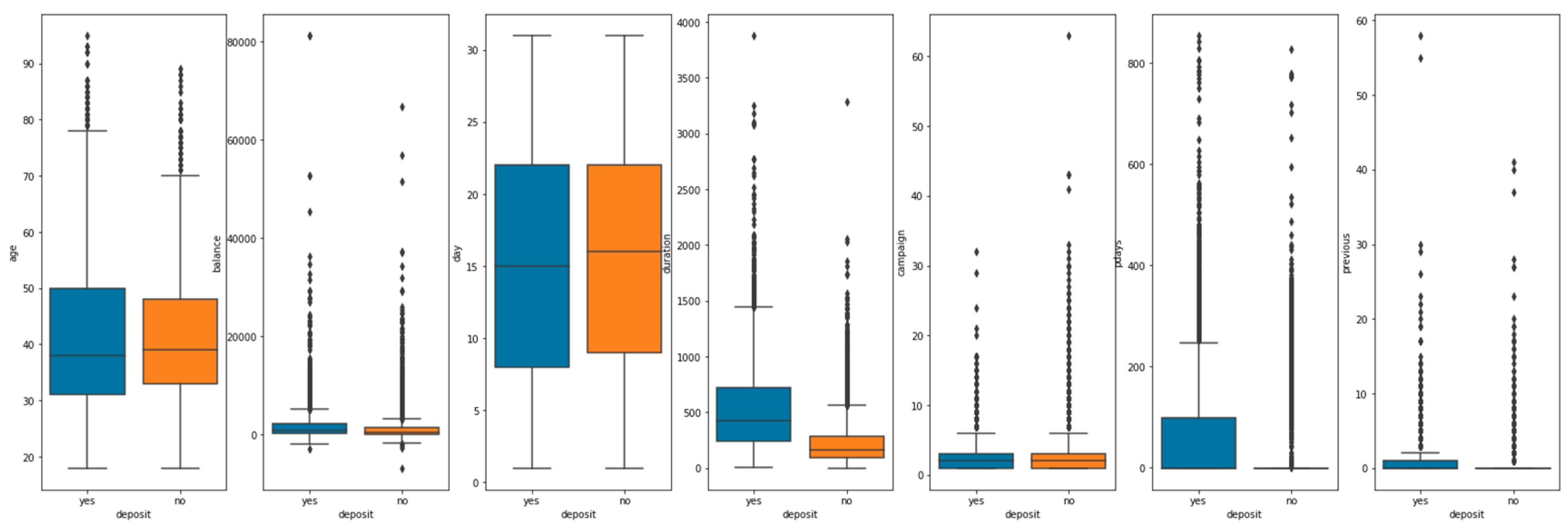
The visualization of numerical data is shown in Figure 2.
There is little difference in the age distribution of whether the two types of customers are successful or not. The balance distribution, day distribution and campaign distribution are also similar. However, the duration distribution, pdays distribution, and previous distribution are significantly different in terms of whether to lend money or not.
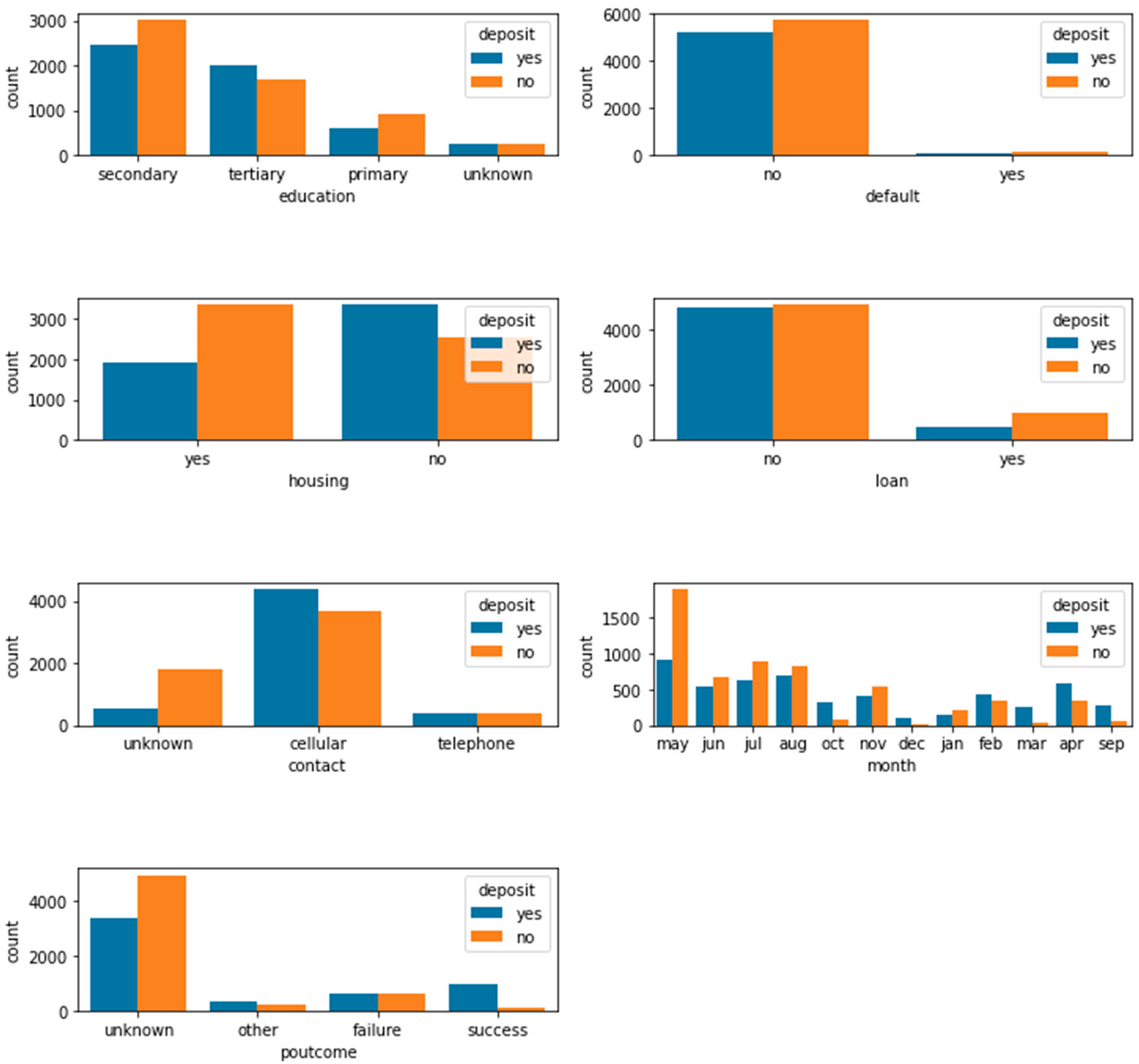
Furthermore, the visualization of categorical data is shown in Figure 3.
The visibility map provides an initial insight into whether these characteristics affect the success or failure of the loan. Plots above convey following things about the dataset:
(1) Job: Among those who applied for loans, about 1/4 worked in management, about 1/6 in blue-collar jobs, and the rest are in a variety of jobs. People who work in management are more likely to succeed in loans.
(2) Martial: 3/5 of the population in the dataset is Marred. Although the majority of people are married, the success rate of loans is slightly lower than that of single people.
(3) Education: The higher the education level, the higher the loan success rate.
(4) Default: Most people in this dataset are not in default, and the number of successful borrowers is slightly lower than the number of failed borrowers.
(5) Housing: Obviously, it's easier to get a loan without a mortgage than with a mortgage.
(6) Loan: Those who have a loan record are more likely to get a loan than those who don't.
(7) Contact: Borrowers who use mobile phones have an easier time getting loans.
(8) Month: The highest rate of loan failures is in January.
(9) Poutput: In the case of a history of borrowing, the result of the last loan has a positive impact on the current loan.

4. Experimental results

4.1. Implementation details

This paper applies the method of machine learning to optimize and predict whether to lend money by learning a large amount of data and relying on previous experience, so that more people who are likely to repay can get loans, and fewer people who cannot repay in the future can get loans.
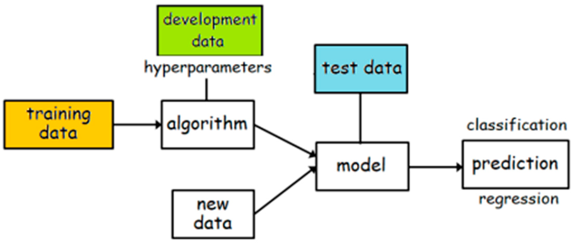
The pipeline of machine learning in loan prediction is shown in Figure 4.

4.2. Training and development

The training data was trained using the random forest algorithm. Then three hyper-parameters are tuned, and used the for loop to find the good ones. These three hyper-parameters are the N_estimators, the max_depth and the min_sample_leaf. The N_estimators show the number of trees in the forest. The max_depth indicates the depth of the trees, also means the number of randomly selected features for each decision tree. And the min_sample_leaf means the number of the branches per layer (leaf’s sample).
This paper searches the parameter firstly set as follows:
n_estimators=500,200,100,50,25,20
max_depth=2,3,4,5,6,7,8,9,10
min_samples_leaf =3,5,7,10,20,30
In the above range, the best results of each parameter are as follows:
best number of estimator=500
best max depth=10
best min samples of leaves=3
After narrowing down the scope, this paper searches parameter sets lastly in the following way:
n_estimators=620,600,580,560
max_depth=10,11,12,13,14
min_samples_leaf =2,3,4,5
The best results of each parameter in this paper are as follows:
best number of estimator=560
best max depth=14
best min samples of leaves=2

4.3. Evaluation

Table 2. Evaluation results on the utilized dataset.
Method Test accuracy F1-score
Random forest 85.62% 85.48%
The confusion matrix is listed in Table 3.

4.4. Result

As can be seen from the table, the prediction performance of random forest classification algorithm is very high. The result of test accuracy was 85.62%, the F1-score (a weighted average of accuracy and recall) was 85.48%.

5. Conclusions

This paper mainly studies the loan prediction in the financial field, and establishes the default prediction model by using the random forest classification method. The random forest adopts Bagging idea and repeated adoption to generate multiple trees and ensure the independence of each tree. Moreover, the random forest method can adjust the weight by itself on the basis of the ground truth value through parameter adjustment, which effectively solves the problem of data classification. The experimental results reveal that the classification performance of the random forest model is very good, and the prediction accuracy can reach more than 85%. It is significant in terms of reference for loan prediction in the monetary field. However, this paper only researches the random forest algorithm in loan prediction. Although the accuracy of this method is quite high, there is a kind of integrated thinking of the decision tree model is also very worth exploring, that is GBDT (Gradient Boosting Decision Tree). [6,7,8,9,10] GBDT(also known as MART-Multiple Additive Regression Tree) can be applied to a variety of scenarios and has a high accuracy rate. It is worthy of further study and comparison with random forest algorithm, so that it may be more effective in predicting loan default.

References

  1. Zhang, N.; Chen, Q. P2P loan default prediction model based on TF-IDF algorithm. Journal of Computer Applications 2018, 38, 3042. [Google Scholar] [CrossRef]
  2. Pan, Y.M.; Wang, Y.J.; Lai, M.Z. Credit risk prediction of supply chain financing enterprises based on IG-SVM model. Journal of Nanjing University of Science and Technology (Natural Science Edition) 2020, 44, 117–126. [Google Scholar]
  3. Chen, X.L.; Han, S.W.; Pang, J.H. Default risk prediction of enterprise loan based on machine learning method[J]. Modeling and Simulation 2021, 10, 890–897. [Google Scholar] [CrossRef]
  4. Zhang, J.M.; Zhou, J.J. An empirical credit risk study of SEMs in small loan companies-based on logistic model and probit model[J]. Statistics and Applications 2014, 3, 159. [Google Scholar] [CrossRef]
  5. Wu, Q.; Wang, H.; Yan, X.; Liu, X. MapReduce-based adaptive random forest algorithm for multi-label classification. Neural Computing and Applications 2019, 31, 8239–8252. [Google Scholar] [CrossRef]
  6. Ke, G.; Meng, Q.; Finley, T.; Wang, T.; Chen, W.; Ma, W.; Ye, Q.; Liu, T.Y. Lightgbm: A highly efficient gradient boosting decision tree. Advances in neural information processing systems 2017, 30. [Google Scholar]
  7. Ke, G.; Xu, Z.; Zhang, J.; Bian, J.; Liu, T.Y. DeepGBM: A deep learning framework distilled by GBDT for online prediction tasks. In Proceedings of the 25th ACM SIGKDD International Conference on Knowledge Discovery & Data Mining; 2019; pp. 384–394. [Google Scholar]
  8. Rao, H.; Shi, X.; Rodrigue, A.K.; Feng, J.; Xia, Y.; Elhoseny, M.; Yuan, X.; Gu, L. Feature selection based on artificial bee colony and gradient boosting decision tree. Applied Soft Computing 2019, 74, 634–642. [Google Scholar] [CrossRef]
  9. Son, J.; Jung, I.; Park, K.; Han, B. Tracking-by-segmentation with online gradient boosting decision tree. In Proceedings of the IEEE international conference on computer vision; 2015; pp. 3056–3064. [Google Scholar]
  10. Sun, R.; Wang, G.; Zhang, W.; Hsu, L.T.; Ochieng, W.Y. A gradient boosting decision tree based GPS signal reception classification algorithm. Applied Soft Computing 2020, 86, 105942. [Google Scholar] [CrossRef]
  11. Luan, S.; Zhao, M.; Chang, X.W.; Precup, D. Break the ceiling: Stronger multi-scale deep graph convolutional networks. Advances in neural information processing systems 2019, 32. [Google Scholar]
  12. Luan, S.; Hua, C.; Lu, Q.; Zhu, J.; Zhao, M.; Zhang, S.; Chang, X.; Precup, D. Revisiting heterophily for graph neural networks. Advances in neural information processing systems 2022. [Google Scholar] [CrossRef]
  13. Luan, S.; Zhao, M.; Hua, C.; Chang, X.W.; Precup, D. Complete the missing half: Augmenting aggregation filtering with diversification for graph convolutional networks. NeurIPS 2022 New Frontiers in Graph Learning Workshop (oral). 2020. [Google Scholar]
  14. Luan, S.; Zhao, M.; Hua, C.; Chang, X.W.; Precup, D. Complete the Missing Half: Augmenting Aggregation Filtering with Diversification for Graph Convolutional Neural Networks. arXiv 2022, arXiv:2212.10822. [Google Scholar] [CrossRef]
  15. Luan, S.; Hua, C.; Lu, Q.; Zhu, J.; Zhao, M.; Zhang, S.; Chang, X.; Precup, D. Is Heterophily A Real Nightmare For Graph Neural Networks To Do Node Classification? arXiv 2021, arXiv:2109.05641. [Google Scholar] [CrossRef]
  16. Luan, S.; Hua, C.; Lu, Q.; Zhu, J.; Zhao, M.; Zhang, S.; Chang, X.; Precup, D. Is Heterophily A Real Nightmare For Graph Neural Networks on Performing Node Classification? 2021. [Google Scholar]
  17. Hua, C.; Luan, S.; Zhang, Q.; Fu, J. Graph Neural Networks Intersect Probabilistic Graphical Models: A Survey. arXiv 2022, arXiv:2206.06089. [Google Scholar] [CrossRef]
  18. Zhao, M.; Liu, Z.; Luan, S.; Zhang, S.; Precup, D.; Bengio, Y. A consciousness-inspired planning agent for model-based reinforcement learning. Advances in neural information processing systems 2021, 34, 1569–1581. [Google Scholar] [CrossRef]
  19. Luan, S.; Zhao, M.; Chang, X.W.; Precup, D. Training matters: Unlocking potentials of deeper graph convolutional neural networks. arXiv 2020, arXiv:2008.08838. [Google Scholar] [CrossRef]
  20. Luan, S.; Hua, C.; Lu, Q.; Zhu, J.; Chang, X.W.; Precup, D. When Do We Need GNN for Node Classification? arXiv 2022, arXiv:2210.16979. [Google Scholar] [CrossRef]
  21. Luan, S.; Hua, C.; Xu, M.; Lu, Q.; Zhu, J.; Chang, X.W.; Fu, J.; Leskovec, J.; Precup, D. When Do Graph Neural Networks Help with Node Classification: Investigating the Homophily Principle on Node Distinguishability. arXiv 2023, arXiv:2304.14274. [Google Scholar] [CrossRef]
  22. Hua, C.; Luan, S.; Xu, M.; Ying, R.; Fu, J.; Ermon, S.; Precup, D. MUDiff: Unified Diffusion for Complete Molecule Generation. arXiv 2023, arXiv:2304.14621. [Google Scholar] [CrossRef]
  23. Hua, C.; Luan, S.; Fu, J.; Precup, D. Multi-Dataset Multi-Task Framework for Learning Molecules and Protein-target Interactions Properties.
  24. Zhao, M.; Luan, S.; Porada, I.; Chang, X.W.; Precup, D. META-Learning State-based Eligibility Traces for More Sample-Efficient Policy Evaluation. arXiv 2019, arXiv:1904.11439. [Google Scholar] [CrossRef]
  25. Luan, S.; Chang, X.W.; Precup, D. Revisit Policy Optimization in Matrix Form. arXiv 2019, arXiv:1909.09186. [Google Scholar] [CrossRef]
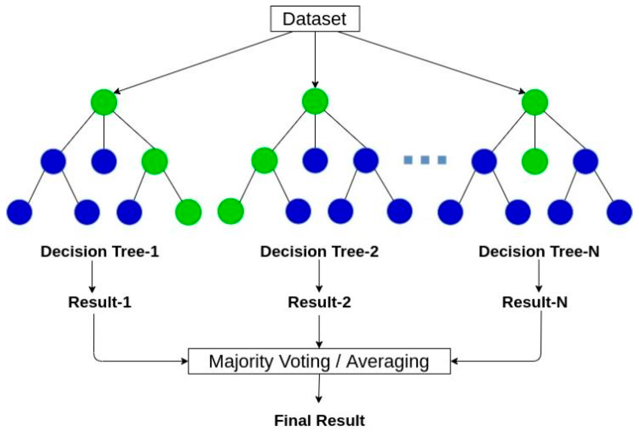
Figure 1. Schematic diagram of random forest.
Preprints 77345 g001
Figure 2. Visualization of numerical data.
Preprints 77345 g002
Figure 3. Visualization of categorical data.
Preprints 77345 g003
Figure 4. Overall framework of loan prediction.
Preprints 77345 g004
Table 1. Data description of the utilized dataset.
Idx Name of variables Description of variables type
1 Age Age int64
2 Job Types of occupation object
3 Marital Marital status object
4 Education Level of education object
5 Default Default record object
6 Balance The average account balance per year int64
7 Housing Whether the individual has a home loan object
8 Loan Whether the individual has a loan record object
9 Contact The way to communicate with customers object
10 Day Day(date) of last contact int64
11 Month Month(date) of last contact object
12 Duration The length of the last contact int64
13 Campaign The number of times the customer was communicated in this activity int65
14 Pdays How long has it been since the last time the client was contacted by the last campaign int66
15 Previous The number of times you communicated with the customer prior to this event int67
16 Poutcome The results of the last campaign object
17 Deposit Predict whether to lend to a borrower object
Table 3. Confusion Matrix of the proposed method.
Predicted True 0 1 All
0 967 208 1175
1 113 945 1058
All 1080 1153 2233
Disclaimer/Publisher’s Note: The statements, opinions and data contained in all publications are solely those of the individual author(s) and contributor(s) and not of MDPI and/or the editor(s). MDPI and/or the editor(s) disclaim responsibility for any injury to people or property resulting from any ideas, methods, instructions or products referred to in the content.
Copyright: This open access article is published under a Creative Commons CC BY 4.0 license, which permit the free download, distribution, and reuse, provided that the author and preprint are cited in any reuse.
Prerpints.org logo

Preprints.org is a free preprint server supported by MDPI in Basel, Switzerland.

Subscribe

© 2024 MDPI (Basel, Switzerland) unless otherwise stated