1. Introduction
Skewness in data is an important feature in various applications. As a typical example, dependence among stock returns is known to be asymmetric in bearish and bullish markets [
1]. To capture such asymmetry, skewed distributions have been extensively studied in the literature. A popular family of skewed distributions is the
skew elliptical distribution [
2], which includes, for example, the
skew-normal distribution [
3] and the
skew-t distribution [
4]. Various measures of asymmetry are also proposed, for example, in [
5,
6,
7,
8,
9] to quantify certain asymmetric feature of an underlying distribution, typically an asymmetry between upper and lower tails.
For a more formal description of the subject of this paper, let
be an
-valued random vector on a fixed atomless probability space. Denote by
H the cumulative distribution functions (cdf) of
with marginal distributions
and
, respectively. For a fixed threshold
, we focus on the following
measure of tail asymmetry (in lower and upper tails) [
9]:
We are also interested in the asymptotic behavior of
as
. Throughout the paper, we assume that
and
are continuous so that
has the unique
copulaC, which is the cdf of
. Then
is a function of the copula given by
where
is the copula of
.
This paper concerns the measure of tail asymmetry (
1) and its asymptotic behavior of the
skew-normal distribution. A
d-dimensional random vector
is said to follow the skew-normal distribution, denoted by
, if it admits the stochastic representation
where
,
is independent of
and
is a set of all
d-dimensional correlation matrices. The parameter
is called the
skewness parameter and
is called the
correlation matrix. The
skew-normal copula, denoted by
, is defined as the copula of
.
The contribution of this paper is twofold. First, we derive an asymptotic formula of the measure of tail asymmetry (
1) in terms of the upper and lower tail orders [
10]. This formula enables us to describe the asymptotic behavior of this measure for the skew-normal copula. Various approaches are also introduced to evaluate the measure (
1) for a finite threshold
. Our second contribution is to numerically demonstrate that, when the correlation or skewness parameters are around at the boundary values, some asymptotic formulas of the skew-normal copula proposed in the literature are not suitable to compute the measure of tail asymmetry with practically extremal thresholds, such as
. This finding supports the use of an exact evaluation of the measure (
1) even for an extremely small threshold
instead of some asymptotic tail approximations proposed in the literature.
Apart from the measure (
1), some other measures of tail asymmetry have been proposed in the literature. Many of these existing measures are based on differences between certain measures of upper and lower tails (see, e.g., [
5,
6,
7,
8]). Such difference-based measures are not appropriate to quantify tail asymmetry of the skew-normal copula since values of these measures tend to be small even for large values of
. On the other hand, the measure (
1) returns reasonable values for such values of
because this measure is based on the ratio between upper and lower tail probabilities. To the best of our knowledge, the measure (
1) is the only ratio-based measure of upper and lower tail probabilities, which seems appropriate to measure the tail asymmetry of the skew-normal copula.
The organization of this paper is as follows. In
Section 2, we review the concept of tail order and skew-normal copulas. In
Section 3, we derive a formula of the measure of tail asymmetry in terms of the upper and lower tail orders. We also explore the measure and its asymptotic behavior for the skew-normal copula. Numerical experiments are provided in
Section 4, where we reveal some situations when some asymptotic formulas of the skew-normal copula proposed in the literature are not appropriate to use .
Section 5 concludes this paper. Detailed calculations and all proofs are deferred to
Appendix A and
Appendix B, respectively.
2. Preliminaries
We begin with introducing some concepts and notations. Two functions are called asymptotically equivalent at , denoted by , , if . A function is called slowly varying at if for any . The set of all slowly varying functions at a is denoted by . Throughout the paper, all vectors in the form , , are understood as column vectors.
2.1. Tail order and tail order parameter
According to [
10], a
d-dimensional copula
C is said to have the
lower tail order if
where
. If, in addition, the limit
exists, then
C is said to have the
lower tail order parameter. The copula
C is called
(lower) tail dependent when
. In this case,
is known as the
(lower) tail dependence coefficient (TDC). The case
is referred to as the
tail independence. When
,
C is said to have
intermediate tail dependence. As such the model (
3) can capture weaker tail dependence that the TDC cannot. Similarly to the lower case,
C is said to have the
upper tail order and the
upper tail order parameter if
where
is such that
.
2.2. The skew-normal copula
Let
follow a
d-dimensional skew-normal distribution defined via the stochastic representation (
2). According to [
3], the joint probability density functions (pdf) of
is given by
where
is the pdf of
and the parameters
and
are specified via
where
The marginal pdf of
,
, is given by
where
and
are pdf and cdf of
, respectively. Note that
,
, where
. Moreover, it follows from (
2) that
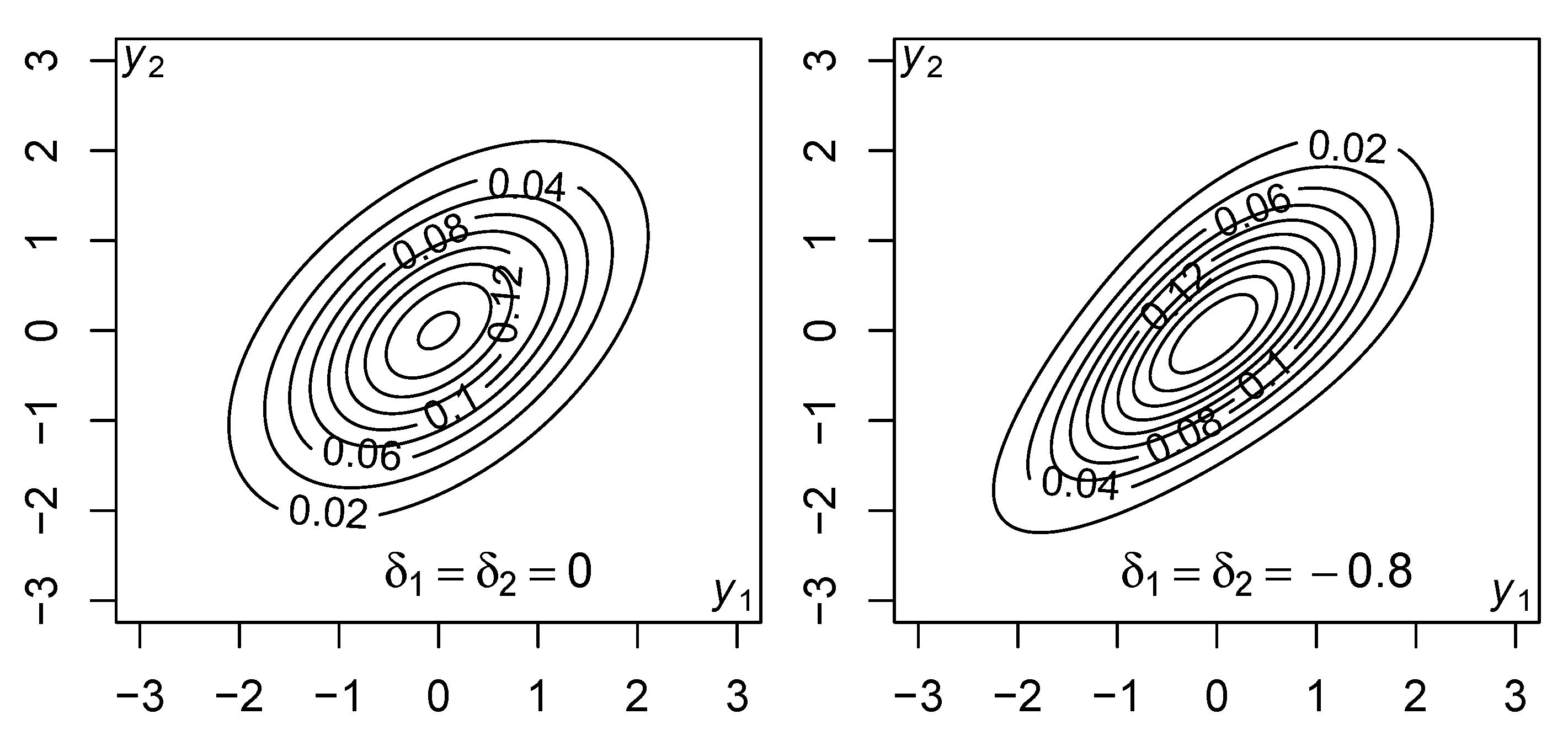
Skewness of the skew-normal copula is illustrated in
Figure 1, where the contour plot of the (symmetric) normal distribution is compared with that of the skew-normal copula with its marginal distributions transformed into the standard normal distributions.
The skew-normal distribution can be written in terms of the conditional distribution of the normal distribution. More precisely, it is shown in ([
3], Section 2.2) that
where
with the
extended correlation matrix
This representation allows us to write the cdfs of
and its copula as follows.
Lemma 1.
Let be the cdf of with marginal cdfs , . Then
where is the cdf of . Therefore, the cdf of the skew-normal copula can be written by
3. Tail asymmetry of the skew-normal copula
In this section we explore tail asymmetry of the skew-normal copula via the measure (
1) and its asymptotic behavior. We will show in Proposition 1 that the measure (
1), after properly scaled, quantifies the difference between the upper and lower tail orders when they differ. Moreover, when the upper and lower tail orders coincide, the measure (
1) quantifies the difference between the upper and lower tail order parameters. These results support the use of the measure (
1) for quantifying tail asymmetry of the skew-normal copula since, to our knowledge, difference-based measures of asymmetry proposed in the literature do not measure tail asymmetry properly when the upper and lower tail indices are not equal.
3.1. Measure of tail asymmetry and tail order
This section explores the relationship between the measure of tail asymmetry (
1) and the tail order. To this end, suppose that a bivariate copula
C satisfies (
3) and (
4).
The next proposition states that the measure of tail asymmetry (
1) can be asymptotically represented in terms of the difference between the upper and lower tail indices.
Proposition 1 (Measure of tail asymmetry and tail order)
. Let C be a bivariate copula with lower and upper tail orders and , respectively. If , then
If and C admits the upper and lower tail order parameters , then
Remark 1 (Relationship with TDCs)
. Equation (13) implies that the limit of as is obtainable from upper and lower TDCs. Indeed, if , and correspond to upper and lower TDCs, respectively. Then is a straightforward calculation from (13). This result can be applied to evaluate the limit of of, for example, the skew-t distribution, whose upper and lower TDCs are available; see [11].
3.2. Measure of tail asymmetry of the skew-normal copula
From this section we focus on the bivariate case
. Let
be the off-diagonal entry of
and
be that of
. We denote, for example, the bivariate case of
by
for notational simplicity. Note that
is the partial correlation of
and
given
, where
and
Y are those used in (
2). By calculation, it holds that
By selecting
and
independently, the range of the parameter
implied by (
14) is given by
Moreover, in the bivariate case, the parameter
is given by
The reader is referred to
Appendix A.1 for detailed derivations of (
14) and (
16).
We first consider the case of a finite threshold
. In this case, the measure of tail asymmetry (
1) of the skew-normal copula can be evaluated by the following proposition. Note that we denote by
the measure (
1) of the skew-normal copula
.
Proposition 2 (Measure of tail asymmetry of the skew-normal copula)
. Let be the skew-normal copula with and . Then its measure of tail asymmetry (1) for a finite threshold is given by
where
The formula (
17) enables us to numerically compute
for a finite threshold
.
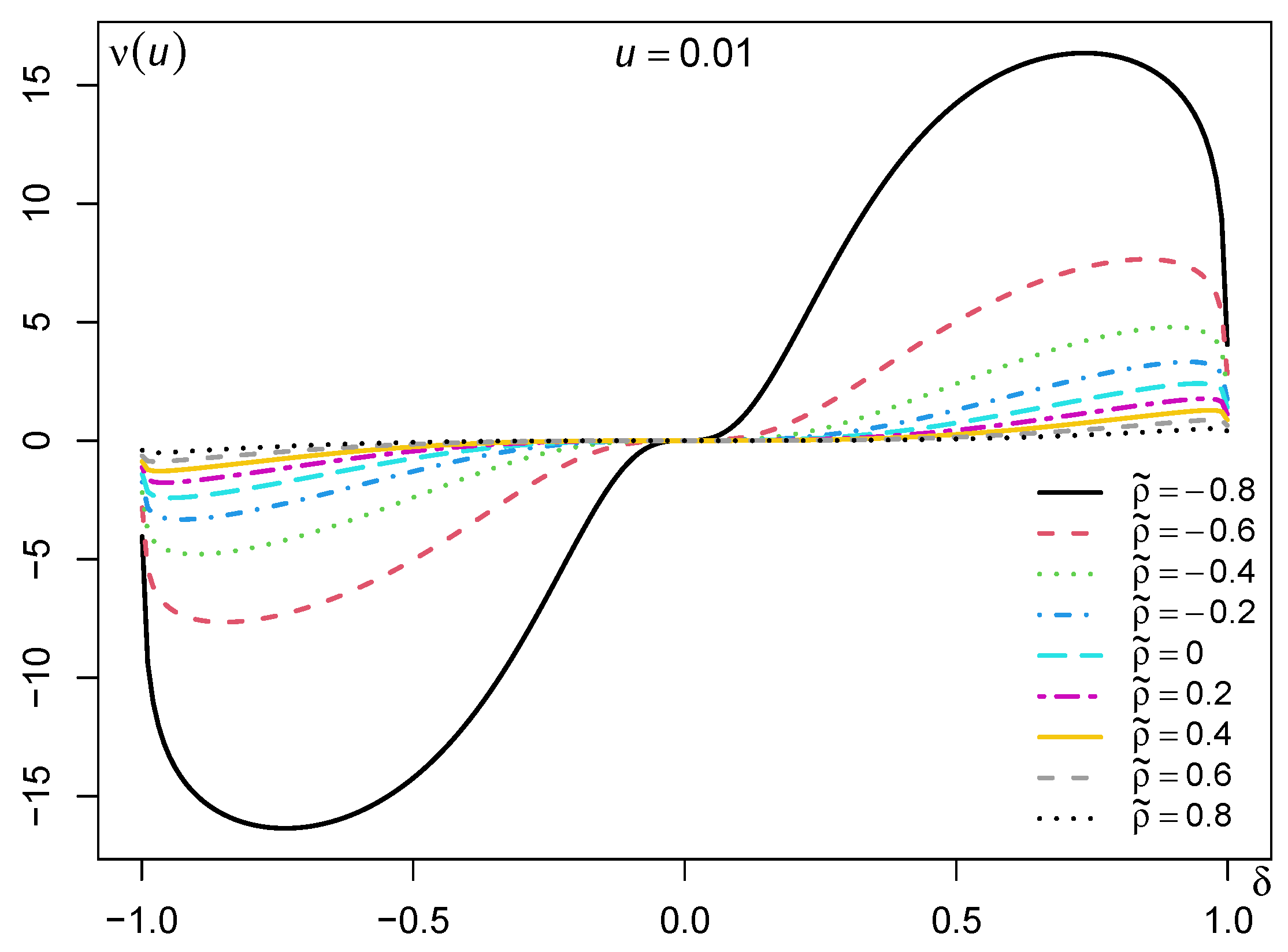
For an illustrative example,
Figure 2 provides curves of
,
, for the skew-normal copula with different parameters. The function
in (
17) is evaluated by
pmvnorm(algorithm = TVPACK) [
12] in the
R package
mvtnorm. We observe that the measure
is symmetric in
with respect to
, and is monotonically changing in
.
We next consider the asymptotic behavior of
for an extremely large and small thresholds. Summarizing the existing results in the literature, we have that
see
Appendix A.2 for detailed calculations. Together wtih
, we obtain the following result.
Proposition 3 (Asymptotic behavior of the measure of tail asymmetry of the skew-normal copula)
. Let be the skew-normal copula with and . Suppose that and have the same sign, which includes the case when at least one of them is zero. Then the measure of tail asymmetry (1) of satisfies
where
Remark 2 (
and
with opposite signs)
. It is assumed in Proposition 3 that and have the same sign. However, the upper and lower tail orders of the bivariate skew-normal copula are investigated in [13] for more general and . Based on their results, analytical expression of the limit can be derived even for and with opposite signs although the expression may not be as simple as (19).
Note that
for every
if
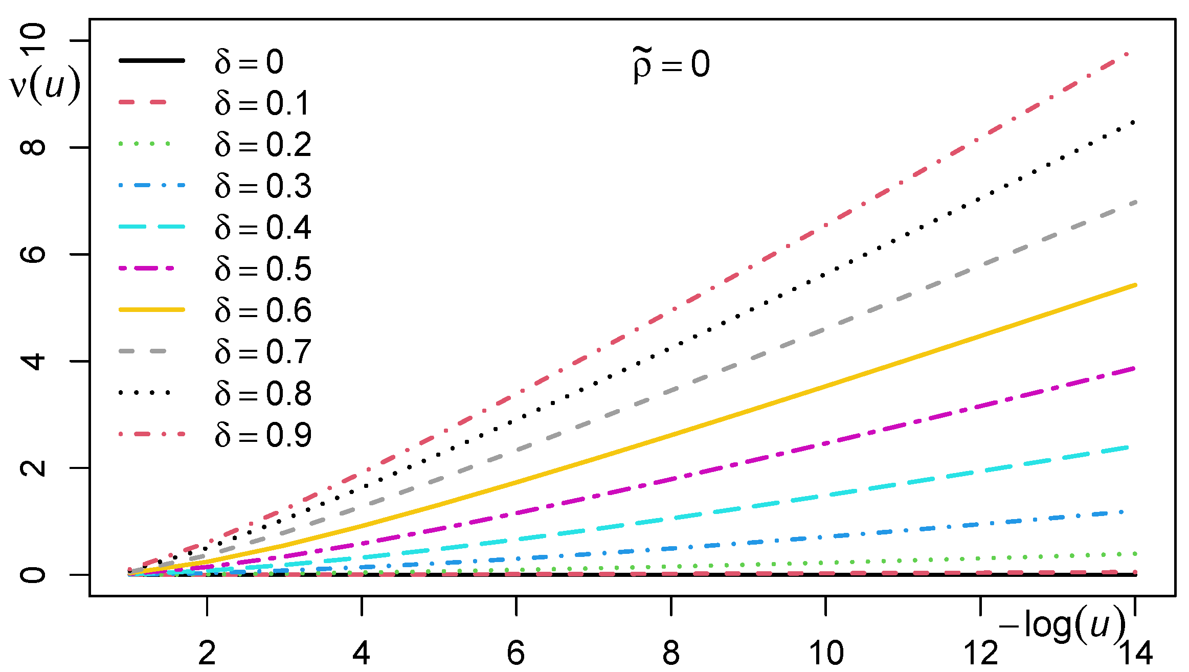
. The asymptotic behavior of
as
is illustrated in
Figure 3, where
is evaluated by (
17) with the algorithm
TVPACK. It is observed that the curves of
against
are asymptotically linear.
Remark 3 (Measure of tail asymmetry and TDCs)
. The measure of tail asymmetry (1) of the skew-normal copula can also be written by
where
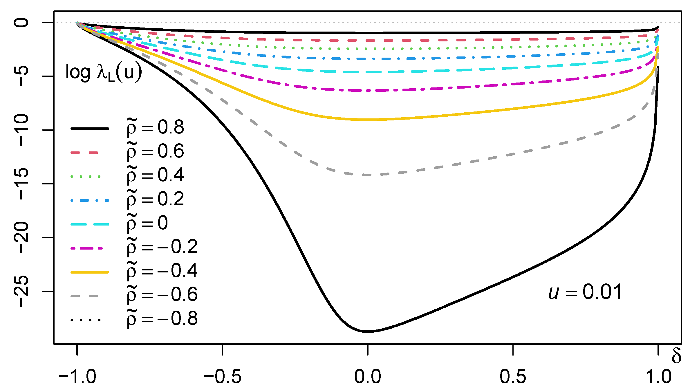
The value for a finite can be computed by (17) with the algorithmTVPACK. Figure 4 shows the curves of against δ for various correlation parameters. It is observed that increases as goes to 1; moreover, is higher for than for .
Remark 4 (Asymptotic formulas of the TDCs).
It is shown in [14] that
Moreover, ([15], Theorem 2) shows that, for ,
where , , and β is defined in (A2) such that .
The following asymptotic formulas of are also given in ([16], Appendix B) based on the tail expansion of the skew-normal copula.
where
Note that the asymptotic formulas in (24) are slightly different from those in (23), but they lead to the same tail order. With this observation, the asymptotic formulas (22), (23) and (24) yield the same limit (19) by using (20).
4. Accuracy of the asymptotic formulas
In
Section 3, various approaches are provided to compute the measure of tail asymmetry of the skew-normal copula. It is partly observed in
Figure 3 that the formula (
17) with the algorithm
TVPACK gives results consistent with the asymptotic formula (
19). As mentioned in Remark 4, the measure of tail asymmetry (
1) can also be computed from the asymptotic formulas (
22), (
23) and (
24) derived in the literature. In line with this, this section explores the performance of these asymptotic formulas in a series of numerical experiments. For ease of illustration, we focus on the equi-skewed case
.
We first compute the value of
for
as an extremely small
u by (
21) and (
11) with
evaluated by
pmvnorm(algorithm = TVPACK) [
12] in the
R package
mvtnorm.
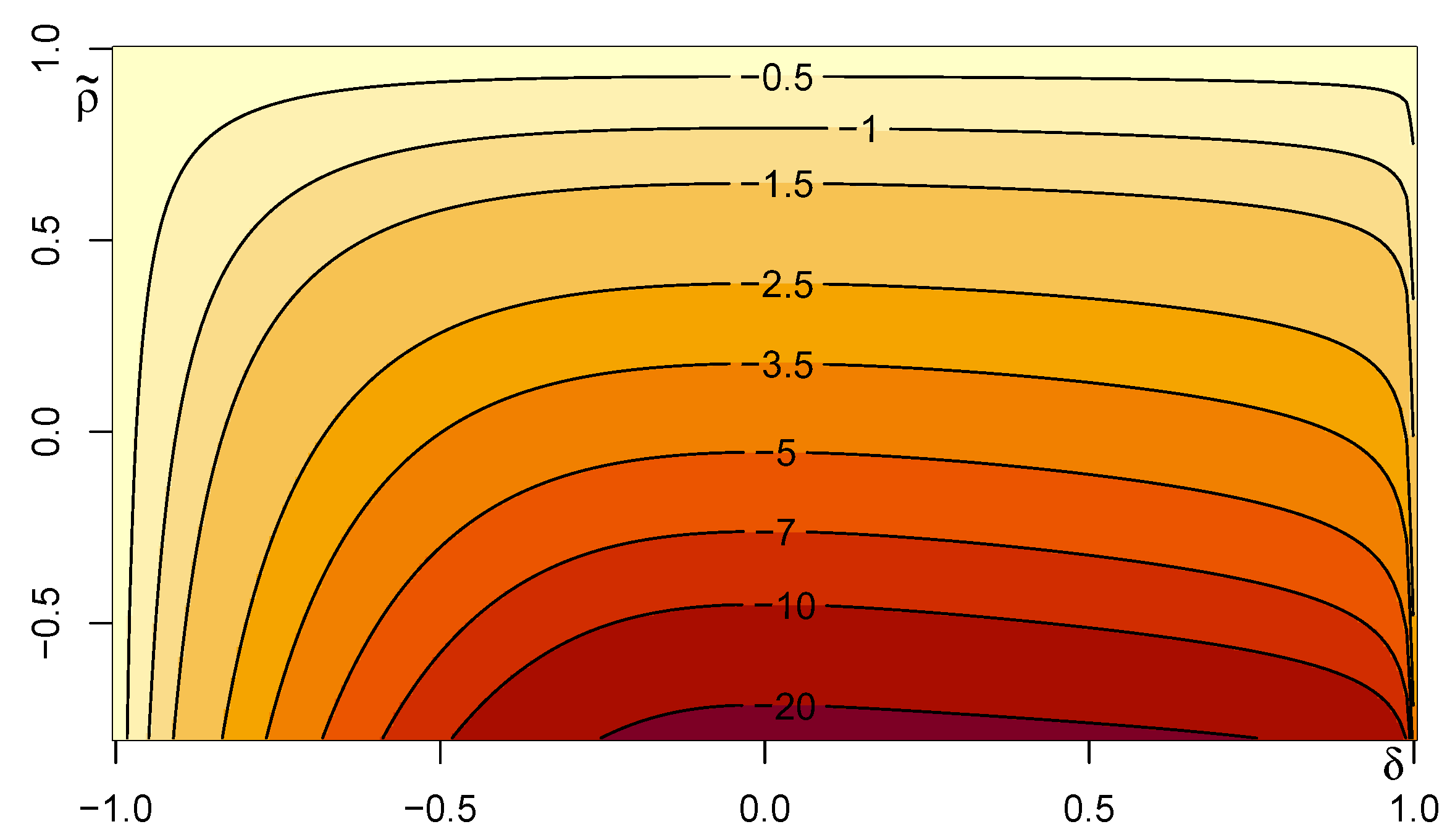
Figure 5 plots the contour of
for
and
by using (
11). The range of
is restricted due to the numerical limitation. We observe that
approaches 0 as
and
go to 1, which is consistent with the fact that the skew-normal copula is comonotonic for these parameters. Monotonicity of the function
with respect to
is also indicated from
Figure 5. Namely, it is observable that the value of
for a fixed
is monotonically decreasing for
and increasing for
, and thus the minimum is attained at
.
For special cases, if
, the correlation between
and
in (
2) is given by
. If
, the correlation is one, the variables are comonotonic, and thus
. If
, the variables are independent and thus
.
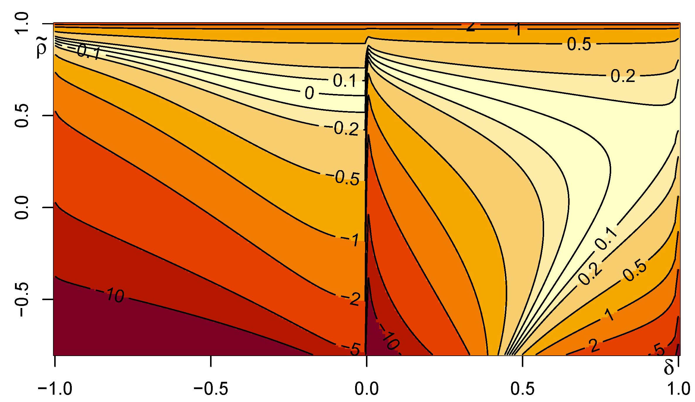
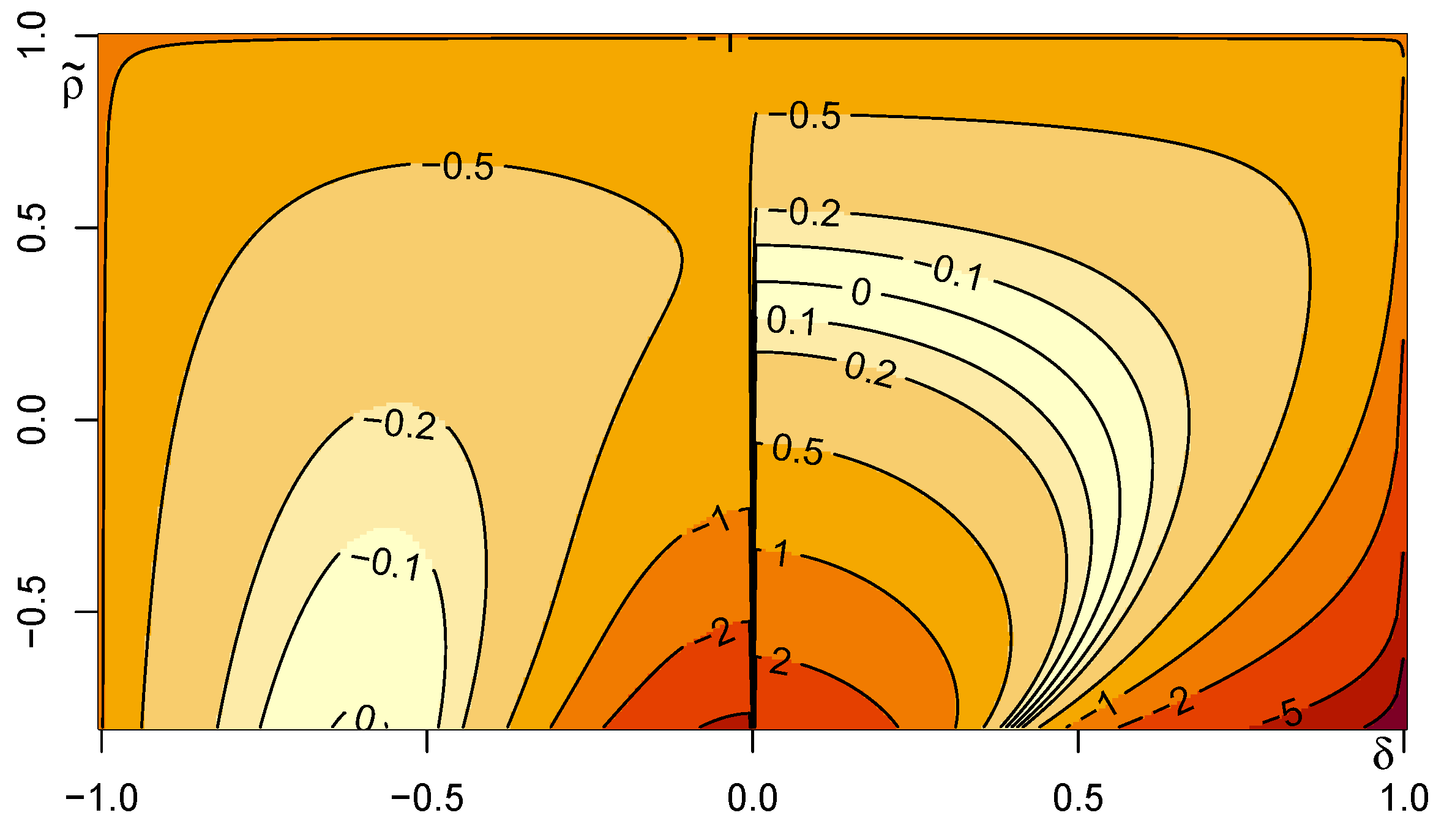
Next, we demonstrate the performance of the asymptotic formulas presented in Remark 4.
Figure 6 plots the contour of the difference of
based on the asymptotic formula (
23) and that based on the numerical evaluation of (
21) with the algorithm
TVPACK. The same plot is provided for the asymptotic formula (
24) instead of (
23). Interestingly, we observe that the two asymptotic formulas perform well on the different areas of the parameter range. In particular, the difference of the asymptotic approximation based on the formula (
23) is large around the boundaries. Discontinuity of the asymptotic formulas is also observed around
, which is more visible for the formula (
23).
5. Conclusion
In this paper we explored the measure of tail asymmetry proposed in [
9], and its asymptotic behavior. We showed that the measure, after properly scaled, is asymptotically equivalent to the difference of the upper and lower tail orders [
10]. Based on this result, we derived an analytical expression of the measure of tail asymmetry for the skew-normal copula. The performance of this formula is verified by comparing it to another analytical formula with a finite threshold. We also investigated the asymptotic formulas of the TDC of the skew-normal copula proposed in the literature. Our numerical experiments revealed that these formulas perform well for moderate values of parameters, but are not recommendable for approximating the measure of tail asymmetry with finite thresholds when the parameters are at their boundaries.
Supplementary Materials
The R code used in this paper is available.
Author Contributions
Conceptualization, Yoshiba; methodology, Yoshiba; software, Yoshiba; validation, Yoshiba, Koike and Kato; formal analysis, Yoshiba, Koike and Kato; investigation, Yoshiba, Koike and Kato; writing—original draft preparation, Yoshiba and Koike; writing—review and editing, Yoshiba, Koike and Kato; visualization, Yoshiba; project administration, Yoshiba; funding acquisition, Yoshiba, Koike and Kato. All authors have read and agreed to the published version of the manuscript.
Funding
This research was funded by JSPS KAKENHI Grant Numbers JP19K23226 and JP21K01581 (Yoshiba), JP21K13275 (Koike), and JP17K05379 and JP20K03759 (Kato).
Data Availability Statement
Not applicable.
Conflicts of Interest
The authors declare no conflict of interest.
Appendix A. Detailed calculations
Appendix A.1. Parameters of the bivariate skew-normal copula
In this section we describe detailed derivations of (
14) and (
16).
For the
correlation matrices
and
, let
and
. Then,
Here,
is the partial correlation of
and
given that
is fixed in the trivariate random vector
given in (
2). By using (
5), we have
where
Hence, we have that
which yields (
14).
Next we check
. By using
we have from () that
Recall that the extended correlation matrix
in (
9) is given by
Since
the parameter
in (
A1) is given by
Note that this representation coincides with that in [16, Appendix B], where
and
are denoted by
and
, respectively. Since
we obtain (
16).
Appendix A.2. Tail orders of the bivariate skew-normal copula
In this section we summarize tail orders of the bivariate skew-normal copula known in the literature. Since
, we study only the lower tail order
,
, for various
. Moreover, we focus on the case when
and
have the same sign, that is, either
or
. In this case, we will show below that the lower tail order is summarized by (
18). The interested reader is referred to [
13] for more general cases of the skewness parameter. Note that the explicit forms of the tail orders of the skew-normal copula can also be found, for example, in [
13,
15,
16]. Although they cover different cases of the parameters, their results are consistent with each other.
Case I: δ 1 =δ 2 =δ
We first consider the equi-skewed case
. It follows from ([
15], Theorem 2) that
where
and
and thus, by calculation,
Note that the signs of
and
are identical, and that
if and only if
. When
, we have that
see also (Li and Joe [
16], Appendix B).
Case II: δ 1 ,δ 2 <0
It is shown in [
13] that
which is also derived in [
16]. Note that the condition
is imposed in [
16], and this condition is implied by (
15). Indeed, we have from (
16) that
and thus the sign of
equals to that of the numerator of the right-hand side of (
A3). From (
15), the inequality
implies that
and thus
.
Case III: δ 1 ,δ 2 >0
It is shown in [
13] that
Note that, in [
13],
and
above are denoted by
and
, respectively. The formula (
A4) is also derived in Appendix B of [
16]. Note again that the condition
imposed in [
16] is implied by (
15). We will check that
that is, the expression (
A4) can be simplified as
First, by multiplying
on the right-hand side of (
A5), the desired equation is equivalent to
which is also equivalent to
by multiplying
on both sides. Since
the left-hand side of (
A6) reduces to
The last two terms of (
A7) are expanded into
By using
, the coefficient of
at the first two terms in the right-hand side of (
A8) is given by
By using
, the last two terms of the right-hand side of (
A8) are rearranged as follows:
Combining (
A9) and (
A10), the term (
A8) reduces to
Therefore, the desired equation (
A6) is now
which can be checked as follows:
Case IV: One of δ 1 and δ 2 is zero and the other is negative
By symmetry, it suffices to consider the case when
and
. In this case, [
13] shows that
.
Case V: One of δ 1 and δ 2 is zero and the other is positive
By symmetry, it suffices to consider the case when
and
. In this case, [
13] shows that, if
, then
The condition
is always satisfied since
and
by (
15). Since
and
, we have that
Appendix B. Proofs
Proof of
Lemma 1. By (
8), it holds that
where
. By (
7), we have
Since
, we obtain (
10).
According to
Sklar’s theorem [
17], the skew-normal copula
has the cdf
Then (
11) follows directly from (
10). □
Proof of
Proposition 1. By (
3) and (
4), we have, as
,
This immediately implies (
13). Notice that the functions
and
are slowly varying at
∞. Together with ([
18], Proposition 2.6 (i)), we obtain (
12). □
Proof of
Proposition 2.
By (
11), it holds that
which completes the proof. □
Proof of
Proposition 3. By (
A11), it holds that
Then the formula (
19) follows directly from (
12) in Proposition 1 and the detailed calculations provided in
Appendix A.2, which is also summarized in (
18). □
References
- Ang, A.; Chen, J. Asymmetric correlations of equity portfolios. Journal of Financial Economics 2002, 63, 443–494. [Google Scholar] [CrossRef]
- Azzalini, A. The Skew-Normal and Related Families; Cambridge University Press: Cambridge, 2014. [Google Scholar] [CrossRef]
- Azzalini, A.; Dalla Valle, A. The multivariate skew-normal distribution. Biometrika 1996, 83, 715–726. [Google Scholar] [CrossRef]
- Azzalini, A.; Capitanio, A. Distributions generated by perturbation of symmetry with emphasis on a multivariate skew t-distribution. Journal of the Royal Statistical Society Series B 2003, 65, 367–389. [Google Scholar] [CrossRef]
- Nikoloulopoulos, A.K.; Joe, H.; Li, H. Vine copulas with asymmetric tail dependence and applications to financial return data. Computational Statistics & Data Analysis 2012, 56, 3659–3673. [Google Scholar] [CrossRef]
- Dobric, J.; Frahm, G.; Schmid, F. Dependence of Stock Returns in Bull and Bear Markets. Dependence Modeling 2013, 1, 94–110. [Google Scholar] [CrossRef]
- Rosco, J.; Joe, H. Measures of tail asymmetry for bivariate copulas. Statistical Papers 2013, 54, 709–726. [Google Scholar] [CrossRef]
- Krupskii, P. Copula-based measures of reflection and permutation asymmetry and statistical tests. Statistical Papers 2017, 58, 1165–1187. [Google Scholar] [CrossRef]
- Kato, S.; Yoshiba, T.; Eguchi, S. Copula-based measures of asymmetry between the lower and upper tail probabilities. Statistical Papers 2022, 63, 1907–1929. [Google Scholar] [CrossRef] [PubMed]
- Hua, L.; Joe, H. Tail order and intermediate tail dependence of multivariate copulas. Journal of Multivariate Analysis 2011, 102, 1454–1471. [Google Scholar] [CrossRef]
- Fung, T.; Seneta, E. Tail dependence for two skew t distributions. Statistics & Probability Letters 2010, 80, 784–791. [Google Scholar] [CrossRef]
- Genz, A. Numerical computation of rectangular bivariate and trivariate normal and t probabilities. Statistics and Computing 2004, 14, 251–260. [Google Scholar] [CrossRef]
- Fung, T.; Seneta, E. Tail asymptotics for the bivariate skew normal in the general case. math.ST 2210.01284, arXiv, 2022.
- Coles, S.; Heffernan, J.; Tawn, J. Dependence measures for extreme value analyses. Extremes 1999, 2, 339–365. [Google Scholar] [CrossRef]
- Fung, T.; Seneta, E. Tail asymptotics for the bivariate skew normal. Journal of Multivariate Analysis 2016, 144, 129–138. [Google Scholar] [CrossRef]
- Li, X.; Joe, H. Estimation of multivariate tail quantities. Computational Statistics & Data Analysis 2023, 185, 107761. [Google Scholar] [CrossRef]
- Nelsen, R.B. An Introduction to Copulas; Springer: New York, 2006. [Google Scholar] [CrossRef]
- Resnick, S.I. Heavy-Tail Phenomena: Probabilistic and Statistical Modeling; Springer Series in Operations Research and Financial Engineering; Springer: New York, NY, 2007. [Google Scholar] [CrossRef]
|
Disclaimer/Publisher’s Note: The statements, opinions and data contained in all publications are solely those of the individual author(s) and contributor(s) and not of MDPI and/or the editor(s). MDPI and/or the editor(s) disclaim responsibility for any injury to people or property resulting from any ideas, methods, instructions or products referred to in the content. |
© 2023 by the authors. Licensee MDPI, Basel, Switzerland. This article is an open access article distributed under the terms and conditions of the Creative Commons Attribution (CC BY) license (http://creativecommons.org/licenses/by/4.0/).
