
Submitted:
25 June 2023
Posted:
26 June 2023
You are already at the latest version
Abstract
In econometrics and finance, volatility modelling has long been a specialised field for addressing a variety of issues pertaining to the risk and uncertainties of an asset. This study presents a robust framework, through a step-by-step design, that is relevant for effective Monte Carlo simulation (MCS) with empirical verifications to estimate volatility using the Generalized Autoregressive Score (GAS) model. The framework describes an organised approach to the MCS experiment that includes "background (optional), defining the aim, research questions, method of implementation, and summarised conclusion". The method of implementation is a workflow that consists of writing the code, setting the seed, setting the true parameter a priori, data generation process, and performance assessment through meta-statistics. Among the findings, it is experimentally demonstrated in the study that the GAS model with a lower unconditional shape parameter value can generate a dataset that adequately reflects the behaviour of financial time series data, relevant for volatility estimation. This dynamic framework is intended to help interested users on MCS experiments utilising the GAS model for reliable volatility calculations in finance and other areas.
Keywords:
consistency
; efficiency
; score driven model
; simulation design
; time-varying parameter estimation
1. Introduction
In finance and econometrics, modelling of volatility has long been used to address a variety of issues concerning the risk and uncertainties of an asset [1,2]. This study is an extension of an earlier study on volatility estimation through the Generalized Autoregressive Conditional Heteroscedasticity (GARCH) model created by Bollerslev [3] (see Samuel et al. [4]). That is, the GARCH model was used in our earlier study to begin a "simulation framework for volatility estimation" work that was introduced in Samuel et al. [4] with the Monte Carlo simulation (MCS) design and guidelines. The Generalized Autoregressive Score (GAS) model is used in this instance to extend the robust design process. As a result, this study identifies a vital framework that is pertinent to the simulation of financial time series data for volatility estimation using the GAS model. The framework can be applied for volatility estimation in financial and non-financial areas.
The GAS is a dynamic model used for time-varying parameter modelling, much like the GARCH model (see [5]). Hence, this study’s main contribution is to show how the GAS model using the GAS package can be effectively applied to enhance time varying scale parameter (volatility) estimation through MC simulation, with empirical verification. Moreover, simulation through any model largely revolves around generating an appropriate dataset that can produce a reasonable output approximation. Thus, one further contribution of this study is to investigate how to use the GAS model to generate (simulate) a dataset that can adequately reflect the behaviour of financial time series data that is relevant for volatility estimation.
MCS studies are computer-based experiments that involve the use of known probability distributions for creating data by pseudo-random sampling. The data may be simulated through parametric models or repeated resampling [6]. MCS is used for approximating real-life scenarios, where it uses random quantities (or a probabilistic approach) to provide deterministic outcomes [7]. Since its introduction by three scientists in the field of physics [8], MCS has become an increasingly applied technique in a wide range of fields including finance, supply chain, engineering, science [9], and in all portfolio and investment types [10]. One of the reasons for its wide applications is because it is based on the concept of the central limit theorem where the distribution of its estimates follows (or converges to) the Normal distribution [11].
The raw data used for this study are the daily closing Standard & Poor South African sovereign bond index, abbreviated S&P SA bond index. They are the bond market’s data in US Dollars from Datastream [12] for the period 4th January 2000 to 11th June 2021 with 5598 observations. The period under study includes the covid-19 pandemic crisis period that began in 2020. The rest of this paper is structured as follows: Section 2 reviews the theories underlying the GAS model, the true parameter recovery (TPR) measure, and the description of the simulation design. Section 3 shows how the simulation framework is illustrated using financial bond return data, with empirical verifications. Section 4 discusses the main findings and Section 5 presents concluding remarks on the novelty of the study.
2. Materials and Methods
2.1. The GAS Model
Volatility can be effectively estimated through a Score Driven (SD) model known as the GAS introduced by Harvey [13] and Creal et al. [14] (see [5,15,16]). The GAS model is also called the Dynamic Conditional Score (DCS) model, and its applications are used in many financial econometrics analytics (see [17]). It provides a connection between the stochastic volatility (SV) models [18] and GARCH models (see [19]).
The GAS model uses the score of the conditional density function to determine the time-variation in the parameters, i.e., the use of the score function is applied as the driver of the parameters’ time variation. Also, the score functions are robust to outliers because they discount extreme values by reducing the number of extreme observations, which takes place because the GAS model is conditional on time t [13]. For instance, if errors are modelled using fat-tailed innovations under a GAS model, a big absolute return swing will not lead to a large increase in volatility [14]. Hence, the GAS model is indeed robust and quite suitable for modelling skewed and/or fat-tailed time series data like financial returns [13,20]. Moreover, like the other observation-driven models, likelihood estimation using the GAS model is simple and direct [5]. Observation-driven modelling exist in the presence of time-varying parameters, where parameters are functions of lagged dependent variables, concurrent variables and lagged exogenous variables (see [14,21] for details).
Let a random vector of M-dimension at time t with a conditional distribution be represented by ∈ such that:
where ≡ are the past time-values of up till , that indicate the set of information available prior to time t [22], and ∈⊆ is a time-varying parameters’ vector with complete characterization of depending only on and a group of additional time-invariant parameters , such that . The key attribute of GAS models is that the score of the conditional distribution (i.e., the conditional probability density function of , as stated in Equation 1) drives the evolution in the time-varying parameter vector , in relation to an autoregressive element:
where is the innovation term denoting a possibly scaled score of with respect to , estimated in (see [14,15,23]). The intercept , vectors and are proper dimensional matrices of coefficients that control for the time-varying parameters’ evolution [5,15]. These are functions of the static parameters vector , that is = (, , [14,17,23]. Various classes of observation-driven models can be obtained with different choices of the scaled score , hence these types of models are referred to as score-driven models [22]. The autoregressive Equation (2) that acts as a mechanism for updating can be generally stated (see [14]) as:
The is a vector relative to the score of Equation (1):
For any realized observation , the time-varying is updated to the next period using Equation (3) with as defined in Equations (4) and (5) [14]. The matrix denotes an I × I (valued) positive definite scaling matrix identified at time t, and:
represents the score of Equation (1) estimated at . The variance of can be accounted for by setting the (scaling matrix) to a power of the inverse of the Information Matrix, , of the time-varying parameters [5,14], i.e.,
with the expectation taken on . For , values can be taken in the set . If = or = 1 is fixed by a user, the inverse of the square root of the conditional score ) pre-multiplies the conditional score’s covariance matrix . However, when = 0, there will be no scaling since = (identity matrix). It should be noted that for any choice of , follows a Martingale Difference with respect to the distribution of since the score’s expectation is zero, that is, E [] = 0 ∀t. More so, we can easily derive the additional moment condition [] = when = [5]. Because is a Martingale Difference, the time-varying parameters’ process can revert to the mean near its long-term value of mean once the spectral radius of . This means that the I-valued vector controls for the level, while the I × I matrix controls for the persistence of the process [5,22]. In Equation (2), the extra matrix of ’s coefficients of the scaled score controls the effect of on , where indicates the direction for updating the parameters vector from to [5,14].
2.1.1. Reparameterisation of the Time-Varying Parameter
The parameter vector in Equation (2) is unbounded because it has a linear specification, and its parameter space is regularly restricted (i.e., ⊂) in practice. Therefore, the GAS structure uses a nonlinear link function , as an alternative to the positivity imposing constraints, to map the reparametrised parameters vector ∈ into such that ∈ also provides a linear effective specification experienced in Equation (2). Based on this, the updating equation now takes the GAS recursion of the form:
where ≡ represents the vkappa vector, , and is a mapping function [5,16]. The estimated coefficients {, , , {, , } and {, , } are the elements of vectors , and respectively, where , , and are the location, scale and shape parameters in that order. The initialisation of the process is at , and , where is the score of Equation (1) with respect to (further details on this can be found in [5,16]).
Based on the dependence of the driving mechanism in Equation (3) on the scaled score vector in Equation (4), Equations (1) to (5) describe the GAS model of p and q as GAS(), and the candidate model GAS is used for the time-varying scale parameter, or volatility, estimation in this study. This is because the time varying parameter evolves in the form of an autoregressive (AR) process of order 1 [23], and the model typically features as GAS [24]. Hence, GAS model is used as the data generating process (DGP) for the simulation modelling, and it also serves as the only candidate model for the empirical data modelling. The volatility persistence of the GAS model is defined as (see [5,14]). Volatility persistence is a measure of how fast the existing shock to volatility will fade away [25] and revert to the mean (normal) state.
The maximum likelihood estimation (MLE) of can be implemented through the prediction error decomposition, given the static parameter vector and the past information . That is, for a sample of N realisations of , gathered in , the MLE of the vector of parameters is a solution of:
with , and the time-varying parameters’ vector for , such that depends on and .
2.2. The True Parameter Recovery Measure
The true parameter recovery (TPR) measure in Equation (10) was developed by Samuel et al. [4] as a means of measuring the performance of the MCS estimator in recovering the true parameter. It is used as a proxy for the coverage of the MCS experiment to determine how much of the true parameter is recovered by the MC simulation estimator.
where is the true data-generating parameter, K = 0, 1, 2, …, 100 is the nominal recovery level, and is the estimator from the simulated data. For instance, a TPR estimated value of 95% or 100% indicates that the MCS estimator recovers 95% or 100% of the true parameter. A full recovery of the true parameter can be achieved by the MCS estimator when = , where , such that the TPR output equals the given nominal recovery level K (i.e., TPR = K%).
2.3. Simulation Design
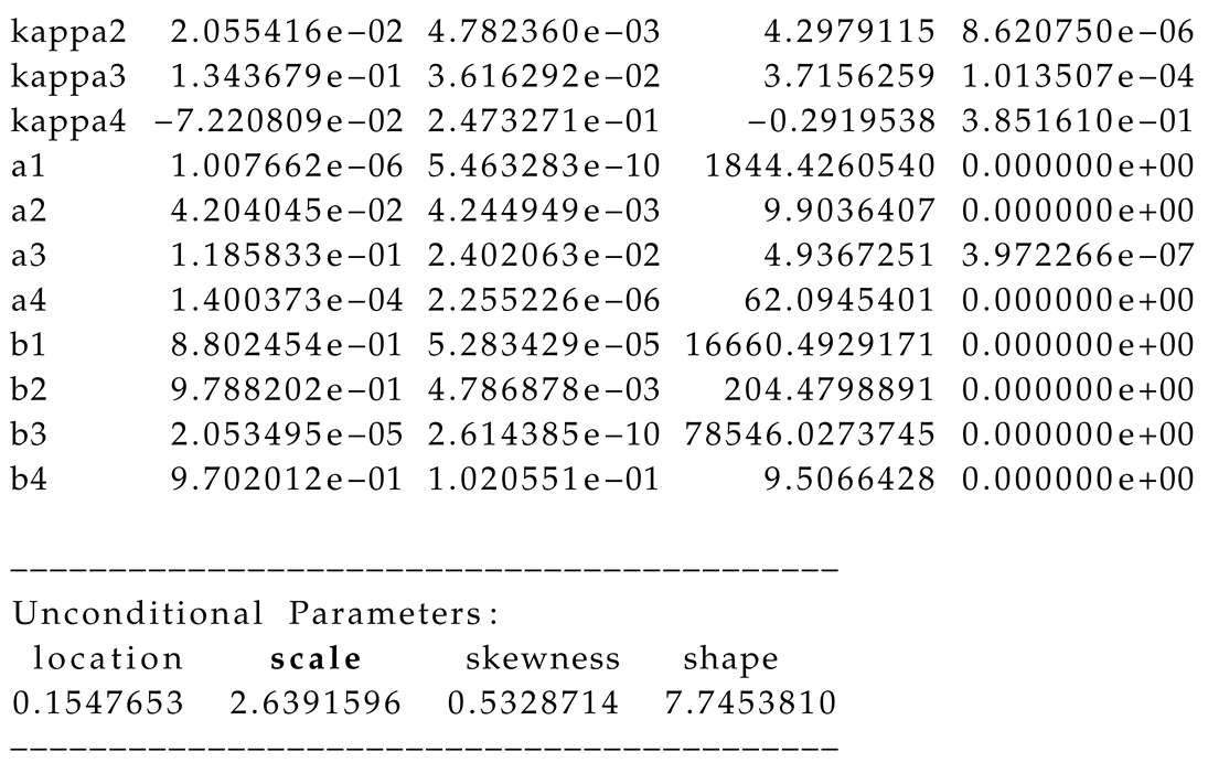
The design of the simulation framework involves "background (optional), defining the aim, research questions, method of implementation, and summarised conclusion". The method of implementation is a workflow that consists of writing the code, setting the seed, setting the true parameter a priori, data generation process, and performance evaluation through meta-statistics (see [4]). These steps, as summarized by the flowchart in Figure 1, are relevant for successful simulations through the GAS model. The details on each design step are as follows:
2.3.1. Aim of the Simulation Study
After optionally stating the background of the study, the next step is to define the aim of the study and it must be concisely, clearly and unambiguously stated for reader’s understanding. The focus of MCS studies generally dwells on estimators’ capabilities in recovering the true parameters , such that E = for unbiasedness, as the sample size for consistency, and root mean square error (RMSE) or standard error (SE) tends to zero as for good efficiency or precision of the true parameter’s estimator. Hence, the aim of the study may revolve around those properties, like the bias or unbiasedness, consistency, efficiency or precision of the estimator. The aim can also evolve from comparisons of multiple entities, like comparing the efficiency of various error distributions, or comparing the performance of multiple models or modification of an existing method.
2.3.2. State the Research Questions
After defining the study aim, relevant questions with regards to the purpose of the simulation should be outlined. These will be pointers to the objectives of the study. The intricacies of some statistical research questions make them better resolved via simulation approaches. Simulation provides a robust procedure for responding to a wide range of theoretical and methodological questions and can offer a flexible structure for answering specific questions pertinent to researchers’ quest [26].
2.3.3. Method of Implementation
The simulation and empirical modelling of this study are implemented in R Statistical Software, version 4.0.3, with RStudio version 2023.03.1+446, using the GAS [5,16], SimDesign [27], tidyverse [28], patchwork [29], aTSA [30], rugarch [31,32], and forecast [33] packages. Computation is executed on Intel(R) Core(TM)i5-8265U CPU @ 1.60GHz 1.80 GHz. The method of implementing the simulation is as follows:
- Write the code: Carrying out a proper simulation experiment that mirrors real-life situation can be very demanding and computationally intensive, hence readable computer code with the right syntax must be ensued. MCS code must be well organised to avoid difficulties during debugging. It is always safer to start with small coding practices, get familiar with them and ensure they run properly with necessary debugging of errors before embarking on more intensive and complex ones. Code must be efficiently and flexibly written and well arranged for easy readability.
- Set the seed: Simulation code will generate different sequence of random numbers each time it is run unless a seed is set [34]. A set seed initialises the random number generator [32] and ensures reproducibility, where the same result is obtained for different runs of the simulation process [35]. The seed needs to be set only once, for each simulation, at the start of the simulation session [6,32], and it is better to use the same seed values throughout the process [6]. The seed is essentially used for reproducibility. Samuel et al. [4] used the GARCH model to show that as the sample size N increases, the arrangement (or pattern) of the seed values generally does not influence the efficiency and consistency of an estimator. This however may depend on the quality of the model used.
-
Next, simulated observations are generated using the true sampling distribution or the true model given some sets of (or different sets of) fixed parameters. Generation of simulated datasets through the GAS model is carried out using the R package "GAS". Random data generation involving this package can be implemented using either of two approaches [5,16]. The first approach is to carry out the data generating simulation directly on a fitted object "fit" (or uGASFit) using the UniGASSim (univariate GAS simulation) function for the simulated random data. The second approach uses the function UniGASSim with "fit = null". This latter approach involves full specification of a GAS model that includes selection of the conditional error distribution of the time series process, and specifying the static parameter = (, , ) that controls the time variation in , as described in Section 2.1.The simulation or data generating process can be run once or replicated multiple times. However, data generation through the GAS process is generally designed to run only once. In their study through autoregressive process, Samuel et al. [4] showed that the outcomes of MCS experiments using the GARCH model are the same for datasets simulated with the same seed value, regardless of whether the simulation or data generating process is run once or replicated multiple times. Hence, the outcome of a single run is the same as the average of multiple runs or replicates. Their findings further revealed that in any multiple generated (simulated) datasets in the family GARCH model, each simulated series is distinct in randomness and shape, and it is different from every other series in the datasets.
- The generated (simulated) data are analysed and the estimates from them are assessed using classic methods through meta-statistics to derive relevant information about the estimators. Meta-statistics (see [27]) are performance measures or metrics for evaluating the modelling outcomes by judging the closeness between an estimate and the true parameter. A few of the frequently used meta-statistical summaries, as described below, include the bias, root mean square error (RMSE), standard error (SE) and relative efficiency (RE). For more meta-statistics, see [6,27,37].
Bias
The bias, on average, measures the tendency of the simulated estimators to be smaller or larger than their true parameter value . It is defined as the average difference between the true (population) parameter and its estimate [38]. The optimal value of bias is 0 [37,39]. An unbiased estimator, on average, yields the correct value of the true parameter. Bias with a positive (negative) value indicates that the true parameter value is over-estimated (under-estimated). However, in absolute values, the closer the estimator is to 0, the better it is. Bias is stated mathematically as , but can be presented in Monte Carlo simulations (see [40]) as . The two formulae are connected as:
where = is a finite number of the sample estimate for the datasets, L is the number of replications, and is the true parameter.
Standard Error
Sampling variability in the estimation can be evaluated via the standard error (SE) as stated (see [40,41]) in Equation (12). Also called Monte Carlo standard deviation, it is a measure of the efficiency or precision of the true parameter’s estimator, where it is used to estimate the long-run standard deviation of for finite repetitions. It does not require knowing the true parameter but depends on its estimator only. The smaller the sampling variability, the more the efficiency or precision of the ’s estimator (see [6]). Sampling variability decreases with increased sample size [37].
RMSE
The root mean square error (RMSE) is an accuracy measure for evaluating the difference between a model’s true value and its prediction. RMSE measure indicates the sampling error of an estimator when compared to the true parameter value [37] and it is stated as:
Its computation involves the true parameter . An estimator with smaller RMSE is more efficient in recovering the true parameter value [37,41], and minimum RMSE produces maximum precision [42]. Consistency of the estimator occurs when RMSE decreases such that as the sample size [6,31]. RMSE is related to bias and sampling variability as:
That is, the RMSE is an inclusive measure that combines bias and SE, such that low SE can be penalised for bias. The mean squared error (MSE) is obtained by squaring the RMSE. MCS is highly dependent on the law of large numbers, and it is expected that the distribution of a suitably large sample should converge to that of the underlying population as the sample size increases [43]. It is also expected that increasing the sample size should relatively decrease the sampling error, but this is not always the case. That is, the number of sample size cannot always be sufficiently increased to limit the sampling error to a bearable level [43]. Using sample sizes between 100 and 7000 inclusive, Kwiatkowski [11] graphically shows the effect of varying sample sizes on simulation outcomes. The author reveals that as the sample size increases, the spread of an estimated value decreases proportionately. However, at some point, additional sample increase does not further reduce the spread [11].
Relative Efficiency
Sampling efficiency between one estimator and the other can be compared using the relative efficiency (RE) statistic by creating ratios between the estimators’ RMSE values as shown in Equation (15). In the formula, the first RMSE or RMSE is taken as the reference estimator, such that other RMSEs are assessed in relation to it. This performance measure can be used when the estimators of interest are unbiased. The RE ≡ 1 when i = 1, and values above (less than) 1 indicate less (greater) efficiency. Less efficiency means more variability than the statistic that is referenced, while greater efficiency indicates less variability and higher precision for recovering the true parameter [37,40]. For instance, suggests that estimator i is the preferred one, i.e., if i = 2 for instance, estimator 1 is less efficient in relation to estimator i = 2 [44].
2.4. Discussion and Summary
After the method of implementation, the last stage in the framework steps is the conclusion, which should reflect a summary discussion of all logical findings from the experiments, with answers to the research questions. The conclusion brings out the novelty of the research and may also include the limitations experienced and opportunities for future work. In addition, relevant information on simulation results can be conveyed through graphics, tabular presentation, or both.
3. Results: Simulation and Empirical
3.1. Practical Illustrations of the Simulation Design: Application to Bond Return Series
By way of illustration, this section practically describes how the stated steps can be applied through Monte Carlo simulations with real data empirical verification. The steps are illustrated using bond returns as follows:
3.2. The Background
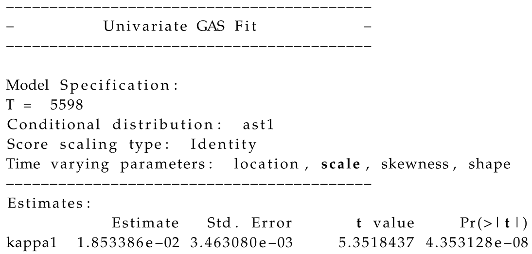
As a preamble, simulation involving the GAS model can be conducted through the UniGASSim function with uGASFit (or simply "fit") object and UniGASSim function with "fit = null" (see Page 52 of Catania et al. [16] for the usage of UniGASSim function). The latter approach using "fit = null" involves full specification of the GAS model, where the coefficients of the matrices , and in Equation (2) have to be defined. Both of these approaches can be done with shape parameter (or degree of freedom) that is time-varying () or constant (). This illustrative study focuses on . In the simulation structure, and matrices are constrained to exist as diagonals, e.g., for a GAS model with Student’s t error distribution, and , where , and are location, scale and shape parameters, respectively. In the outputs of the estimation, a1, a2, a3, b1, b2 and b3 are estimates of , , , , and , respectively (see Appendix A for clues). Also , where is an identity matrix of a suitable size, is the ThetaStar object, and is a mapping function that is represented by the UniUnmapParameters() function1. The ThetaStar is a vector of the unconditional time varying parameters, i.e., , where , , and are the unconditional location, scale and shape parameters, respectively. The coefficients kappa1, kappa2 and kappa3 in the estimation’s outputs are vector ’s elements, where (see Appendix A for clues, and [5] for more details).
It is believed that an observation-driven model can suitably estimate volatility when the underlying error distribution is appropriately assumed [45]. In other words, to minimize risk and adequately maximise asset returns, volatility needs to be estimated with an appropriate error assumption when the true error distribution is unknown. As described in Section 2.1, GAS(1,1) model is used as the true data generating process (DGP) for the MC simulation modelling. Hence, this illustrative study demonstrates the dynamics of the observation-driven model GAS, where the outcomes of the model fitted with each of seven assumed error distributions of the Gaussian, skew-Gaussian, Student’s t, skew-Student’s t, asymmetric Student’s t with one tail decay parameter (AST1), asymmetric Student’s t with two tail decay parameters (AST), and asymmetric Laplace distribution (ALD) are compared to obtain the most suitable for volatility estimation. Details on the error distributions can be seen in [5,14,46] or through the function DistInfo() in R package "GAS".
For further background layout, it is known that financial data are fat-tailed [47], i.e., non-Normal. Hence, to obtain a set of simulated observations that can closely reflect this fat-tailed behaviour of financial time series data under the GAS modelling, the unconditional shape parameter or degree of freedom () needs to be modified. Modification of can only take place within numerical bounds or range 4 to 50.01. That is, the parameter space can take values from 4.01 to 50. Values outside of this range are unacceptable by the UniUnmapParameters() function. This study investigated this with various datasets by using values outside the range and discovered that the outputs only returned "Not a Number (NaN)" for the unconditional location, scale and shape parameters. Readers can check Table 2 on page 14 of Ardia et al. [5] for all the imposed numerical bounds.
Next, this study carries out an experiment with = {10.3, 8.2, 4.1} to determine which will be appropriate to generate simulated observations that properly reflects the fat-tailed behaviour of financial data. This is executed by fitting GAS(1,1)-Student’s t model with time-varying location, scale and shape parameters to the SA bond return data. All the obtained estimates from the fit are then used directly unaltered (except for that is altered or modified) to generate three sets of 30000 simulated datasets. That is, the first dataset is obtained with = 10.3, the second and third with = 8.2 and = 4.1, respectively. For each simulated dataset, a quantile-quantile (QQ) plot is produced as displayed in Figure 2. It can be seen from the figure that the plot in Panel C for GAS(1,1)-Student’s t with = 4.1 displays fatter tails than the other two panels with = 8.2 and = 10.3. The tails of Panel C’s plot is about twice and more than twice as fat as those of Panels B and A, respectively. Hence, the DGP GAS(1,1) model, as stated in Equation (16), fitted to a Student’s t distributed error with of 4.1 is the most suitable among the three to generate the required simulated financial return data.
It is observed in this background study that modification of the using the fit object approach is not directly feasible. Hence, this study applies the fit = null approach, where all the estimates (except the that is modified) from the fit object are used. That is, all the estimates obtained from the fit of the true model to the real bond return data are directly used unaltered, except the modified , in the specification of the GAS simulation process.
The Student’s t is used as the true error distribution for this illustration because it is assumed that financial data appear to have a distribution much like it, and it is also believed that it can suitably deal with fat tailed or leptokurtic features [48,49] experienced in financial data [50]. However, to buttress the illustration, we further used the AST1 as another true error distribution in addition to the Student’s t, and compare their outcomes. Besides these two true sampling errors, users may choose to use any relevant non-Gaussian distributions, as stated in the DistInfo() function, for their data generations based on individual user’s research needs. For any chosen true error distribution, the DistInfo() function reveals the parameter/s that must be specified as time-varying.
3.3. Aim of the Simulation Study
This study aims at obtaining the most appropriate assumed error distribution to use for conditional volatility estimation when the underlying (true) error distribution is unknown.
3.4. Research Questions
This simulation study should result in responses to the following questions:
- 1.
- Which among the assumed error distributions is the most suitable from the GAS simulation process to estimate volatility?
- 2.
- What type (i.e., strong, weak or inconsistence) of consistency, in terms of RMSE and SE, does the volatility persistence estimator of the GAS process exhibit?
- 3.
- How does the estimator of the most suitable assumed error distribution compare to the estimator of contending assumed error distributions with regards to bias, and efficiency (or precision) in terms of RMSE, SE and RE?
- 4.
- How is the performance of the MCS estimator in recovering the true parameter B?
3.5. Method of Implementation
Since we intend to use the Student’s t and AST1 as the true error distributions to generate the simulated observations, the method of implementation is described via two Monte Carlo experiments. The implementation method is illustrated using the UniGASSim function with "fit = null" as discussed in the background. This approach involves full specification of the GAS model in the coefficients of matrices , and . For the two true error distributions, the scale parameters’ descriptions of the conditional volatility are set within and . The is the GAS volatility persistence parameter in the diagonal of matrix (see [14,51]). Moreover, the and parameters of the GAS model actually correspond to the and parameters, respectively, of the GARCH model [51].
Next, the two MCS experiments to illustrate the method of implementation are carried out using each of the two true error distributions one after another.
3.5.1. Method of Implementation with the Student’s t Error
With Student’s t as the true innovation distribution, the written code is first used to fit the true model GAS(1,1)-Student’s t with time-varying (denoted by "TRUE" in the UniGASSpec function) location, scale and shape parameters to the SA bond return data through the UniGASFit function. The time variation in the location, scale and shape parameters of the fit are graphically described as displayed in Figure 3, with the location in the top panel, followed by the scale and then the shape parameter graphics.
Next, through the UniGASSim function, using seed 12345 in the code, the value of the scale parameter b2 = (i.e., 9.830649e) from the fit is set a priori as the true parameter for the MCS process, as shown in Panel A of Table 1. This value and all the other estimates (with the that is modified to 4.1) from the fit object are used in the code to generate (simulate) three sets of N = 30000 observations. That is, all the estimates from the fit of the true model to the real return data are directly used unaltered, except the modified by using 4.1 (in the ThetaStar object of the code) in place of the fit object’s estimate of = 8.17843724.
Next, due to initial values effect in the data generating process which may lead to size distortion [52], the first N = {13000, 12000, 11000} sets of observations are each discarded at each stage of the generated 30000 observations to circumvent such distortion. That is, only the last N = {17000, 18000, 19000} simulated return observations are used under each of the seven assumed error distributions, as shown in Table 1. This trimming steps are carried out following the simulation structure of Feng and Shi [38]. An observation-driven process can be size distorted with regards to its kurtosis, where strong size distortion may be a result of high kurtosis [53]. After generating the simulated return datasets, GAS(1,1) process is fitted to them under each of the seven distributed error assumptions. The full analytic code that shows the lines of commands for each stage of the method of implementation is available from the authors on request.
Next, comparisons through the four meta-statistical summaries comprising the bias, RMSE, SE and RE are carried out for the volatility persistence estimator . The most suitable assumed error distribution for volatility estimation will be obtained from the estimator with the best precision and efficiency (for recovering the true parameter) in the meta-statistical comparisons done under the seven error assumptions.
Now, comparing RMSE for in Panel A of Table 1, the AST1 assumed error distribution outperforms the other six assumed errors, including the true error Student’s t, in efficiency with the least value as N tends to the peak. For bias comparison, the AST1 also outperforms the rest of the error assumptions with the lowest absolute value of bias as N tends to the peak. Comparing SE, the Student’s t, skew-Student’s t, and AST1 are equal in performance for efficiency and precision in terms of SE, and they outperform the rest. The AST assumed error follows them in performance. Lastly, for RE comparison, we used each preceding RMSE as the reference estimator, i.e., RMSE as the reference estimator for RMSE, and RMSE for RMSE under each error assumption. The outcomes show that the AST1 displays the highest precision for recovering the true parameter than the rest, with the smallest RE value as N tends to the peak. The RMSE and SE performance measures also showcase adequate consistency in recovering the true parameter under the seven assumed distributed errors. To summarise, when the true error distribution is Student’s t, the AST1 assumed error distribution relatively outperforms the other six distributed error assumptions in efficiency and precision, and in the overall performance.
Panel A of Table 1 further reveals that the MCS estimator considerably recovers the true parameter B at the 95% (i.e., 0.95) nominal recovery level. The recovery outcomes for each of the seven error distribution assumptions are visually displayed in Figure 4, where it is revealed that the MCS estimates perform considerably well in recovering the true parameter as shown by the closeness of the TPR outcomes to the 95% nominal recovery level. This indicates a good performance of the MCS experiments with considerably valid outcomes. However, the non-Gaussian error assumptions perform better in the recovery than the Gaussian and skew-Gaussian assumed errors, as revealed in the plot. It can also be observed from the results in Panel A of the table that the MCS estimate is directly proportional to the TPR outcome. Hence, the smaller (larger) the MCS estimate, the smaller (larger) the TPR outcome.
3.5.2. Method of Implementation with AST1
The second illustration of the method of implementation is carried out with the AST1 as the true error distribution. The written lines of code is first used to fit the true model GAS(1,1)-AST1 with time varying location, scale, skewness and shape parameters to the SA bond return data through the UniGASFit function. The time variation in these parameters are graphically displayed in Figure 5, with the location in the top panel, followed by the scale, skewness and then the shape parameter graphics downwards in subsequent panels.
Next, through the UniGASSim function, using seed 12345 in the code, the value of the scale parameter b2 = (i.e., 9.788202e) from the fit is used (or set) a priori as the true parameter for the MCS process, as shown in Panel B of Table 1. This value and all the other estimates (with the that is modified to 4.1) from the fit object are used to generate three sets of N = 30000 return observations. In other words, the outputs from the fit are used as arguments for the objects , and ThetaStar (with a modified = 4.1) to generate the simulated observations. That is, all the estimates from the fit of the true model to the real return data are directly used unaltered, except the unconditional shape parameter or degree of freedom value = 7.7453810 that is modified to = 4.1. Next, following the previous trimming pattern, N = {17000, 18000, 19000} datasets are used under each of the seven assumed error distributions, as shown in Table 1. The full code is available from the authors on request.
Now, comparing RMSE and SE for in Panel B of Table 1, the AST1 error assumption outperforms the other six assumed errors in efficiency and precision with the least values as N tends to the peak. For bias comparison, the AST1 also outperforms the rest, with the lowest absolute values of biases as N tends to the peak. The relative efficiency (RE) comparison is not done here due to the weak consistency of the RMSE under the AST and ALD assumed errors. In this study, consistency is termed "strong" ("weak") when the estimator’s RMSE/SE value decreases as the sample size N increases without (with) distortion. To summarise, when the true error distribution is AST1, the AST1 assumed error distribution outperforms the other six error distribution assumptions in efficiency and precision, and in the overall performance. It is also observed from the outcomes of the RMSE and SE for both true models in Panels A and B that the GAS model with the Gaussian error distribution is considerably consistent but not efficient when the true error distribution is not Gaussian.
Furthermore, as revealed in Panel B of Table 1 and as visualised in Figure 6, the MCS estimator considerably recovers the true parameter B at the 95% nominal recovery level, for each of the seven assumed errors. This indicates a good performance of the MCS experiments with considerably valid results. However, as also observed under the true model GAS(1,1)-Student’s t, the non-Gaussian error assumptions perform better in the recovery than the Gaussian and skew-Gaussian assumed errors, as revealed in the plot. Panel B of Table 1 also shows that the closer the MCS estimate is to zero, the smaller the TPR outcome. It can be seen from Figure 4 and Figure 6, and in Table 1 that the MCS estimator performs slightly better at recovering the true parameter under the Gaussian and skew-Gaussian assumed errors for the true model GAS(1,1)-Student’s t than it is for true model GAS(1,1)-AST1. Moreover, the true model GAS(1,1)-Student’s t displays better consistency for the RMSE and SE metrics than the GAS(1,1)-AST1 as revealed in Table 1. Hence, these show the preference of the Student’s t error for the data generation process than the AST1 error.
3.6. Empirical Study
Next, the results of the MCS experiments are now empirically verified using real return data from the SA bond index. Among the seven assumed error distributions, the most appropriate for the GAS process to estimate the volatility of the bond market’s returns is investigated. For the market index, the price data are transformed to the log-daily returns by taking the difference of logarithms of the price, presented in percentage as:
The and are the closing bond price index at time t and the previous day’s closing price at time , respectively; r denotes the current return and ln is the natural logarithm.
3.6.1. Exploratory Data Analysis
To begin with, the price and return series are first examined through exploratory data analysis (EDA) as shown in Figure 7 to Figure 9. The EDA visually inspects the content of the dataset to reveal vital information and possible outliers. The histogram plot in panel A of Figure 7 shows a skewed non-symmetric distribution that suggests non-stationarity in the price index, while panel B reveals approximately symmetric or stationary distribution in the return series. Panel A of Figure 8 also reveals the non-stationarity in the price index as observed in the price series plot, while panel B shows stationarity in the returns through the return series plot. Figure 8 further reveals four obvious extreme spikes in the distributions of price and returns during the period under study. These spikes are a result of severe global events and economic downturns that led to extreme market volatilities, notably the 2002/2003 SARS epidemic outbreak [54], the 2008 global financial crisis caused by the dot.com bubble [55], (another possible cause of the 2008 turmoil was the U.S. loans crisis, i.e., the defaults on consolidated mortgage-backed securities [56]), the 2016 Brexit issues, and the 2020 covid-19 pandemic outbreak. Figure 9 shows the price and return densities in Panels A and B respectively, while Panels C and D display the movements of the price and return distributions with their densities.
3.6.2. Tests for Autocorrelation and Heteroscedasticity
Next, autocorrelation (or serial correlation) is checked by fitting an autoregressive moving average (ARMA(p,q)) model (see [31]), with a non-skew (Normal) innovation distribution and a skew distribution (Student’s t innovation distribution), to the stationary return series. The p and q are the orders of the AR and MA processes, respectively. Student’s t innovation distribution is used because it adequately reflects the distribution of financial data [57]. Among the candidate ARMA(p,q) models examined, both ARMA(1,1) and ARMA(2,2) models as stated in Equations 18 and 19 are found adequate to remove possible serial correlation in the residual returns. The autocorrelation function (ACF) and partial ACF (PACF) plots of the fit of the ARMA(2,2) model is displayed in Figure 102. Table 2 presents the results of the Weighted Ljung-Box (WLB) tests (see [58] for details) on the "standardized" and "standardized squared" residuals for fitting the two models. The p-values of the tests at lag order 9 for ARMA(1,1) and lag order 19 for ARMA(2,2) are all greater than 0.05, under each error distribution. Based on this, we fail to reject the null hypothesis of "no serial correlation" in the SA bond market’s returns.
Through the outcomes from the autocorrelation test, Engle’s ARCH test (see [59]) is carried out using the Lagrange Multiplier (LM) and Portmanteau-Q (PQ) tests to check for the presence of heteroscedasticity in the residuals. These tests are implemented based on the null hypothesis of homoscedasticity in the residuals of an Autoregressive Integrated Moving Average (ARIMA) model. The tests are executed using the arima() function, in R package aTSA, for ARMA(1,1) and ARMA(2,2) models. The outcomes of both tests reveal highly significant p-values of 0 from lag order 4 to 24 as shown in Panels A and B of Table 3. Thus, the null hypothesis of "no heteroscedastic" in the residuals is rejected, which denotes the existence of volatility clustering. Volatility clustering infers that big changes in returns tend to be followed by big changes, of either sign, and small changes tend to be followed by small changes [60]. Based on the outcomes, an autoregressive model can be fitted to filter out the heteroscedasticity in the return series. This is done by fitting the GAS(1,1) model, as shown in Equation (16), with each of the seven error distributions, to the SA bond returns.
3.6.3. Selection of the Most Appropriate Error Assumption
Next, selection of the most appropriate assumed error distribution to describe the market’s returns, when fitted with the GAS model for volatility estimation, is obtained from Table 4. The results of the GAS(1,1) model fitted with each of the seven assumed innovation distributions to a real return data from the SA bond market index is compared with the outcomes of the MCS studies. The empirical outputs through the Akaike information criterion (AIC) and Bayesian information criterion (BIC) (see [31] for details) are presented in Table 4. The error distribution with the least values of the information criteria is selected as the most suitable to describe the market for volatility estimation. It is observed from the table that the GAS parameter estimate () is statistically significant at 1% level under the seven assumed innovation distributions.
The empirical findings are conducted in two ways. The first outcome is in Panel A of Table 4, where the seven assumed errors are compared when the scale parameter alone is time-varying. It is observed here that the values of the AIC and BIC are smallest under the AST1 error distribution. The second outcome is in Panel B where the seven innovation distributions are compared when the location, scale, and shape parameters are time-varying. The results also show that the two information criteria are smallest under the AST1. Hence, the AST1 innovation assumption outperforms the other six assumed innovation distributions. These outcomes are consistent with the results of the MCS studies. The code for the empirical modelling is available from the authors on request.
The empirical outputs of the GAS(1,1)-AST1 model, with time-varying location, scale, skewness and shape parameters, fitted to the SA bond return dataset are given in Appendix A. Hence, using the outputs, the equations of the GAS model for time-varying scale (or volatility), location, skewness and shape parameters can be stated as:
4. Discussion and Summarised Conclusion
In conclusion, it is observed in the MCS studies that using the UniGASSim function with "fit = null" (i.e., full specification of the GAS model) approach, the AST1 consistently emerges as the most suitable assumed error distribution to use with the GAS model for volatility estimation and description of the SA bond returns when the underlying error distribution is unknown. The result was verified empirically. The persistence of volatility () under this most suitable error distribution as revealed in Table 4 is, on the average, 0.98. Precisely, the outcomes are 0.9790 and 0.9818 in Panels A and B of the table, respectively. Hence, this shows that the SA bond market’s returns volatility is quite persistent.
The conclusion proceeds with answers provided to the research questions. For answer to the first question, the AST1 distribution is the most appropriate among the seven assumed error distributions from the GAS process simulation for volatility estimation. Second, the volatility persistence estimator displays considerably strong consistency. To break this down, there is strong consistency for the estimator under all the seven assumed error distributions in the Student’s t true error distribution (or true model GAS(1,1)-Student’s t) for both RMSE and SE in Panel A of Table 1. The AST1 true error distribution, or true model GAS(1,1)-AST1, in Panel B also shows considerably strong consistency under the error assumptions, with the exception of the weak consistency in the AST and ALD assumed errors for RMSE metric, and under the Gaussian assumed error for SE metric. Third, when compared to contending assumed error distributions, the estimator of AST1 is the overall best in efficiency and precision in terms of RMSE, SE and RE, and in absolute values of biases under the two true error distributions, as revealed in Table 1.
Fourth, as a proxy for the coverage of the MCS experiments, the MCS estimator performed well in recovering the true parameter B through the TPR measure for the 95% nominal recovery level as revealed in Table 1. The results show that the TPR results are suitably close to the 95% nominal recovery level under the seven assumed error distributions for the two true error distributions (or true models). This indicates a good performance of the MCS experiments with considerably valid results. However, the non-Gaussian error assumptions performed better in the recovery than the Gaussian and skew-Gaussian assumed errors, for the two true error distributions. The study also observed from the outcomes of the TPR measure and the consistency of the RMSE and SE, that the Student’s t is a preferred error distribution for data generation than the AST1.
This illustrative study through the GAS simulation modelling focused on time-varying shape parameter or degree of freedom , where the "shape = TRUE". Interested users and readers can try the other approach with "shape = FALSE" (i.e., constant shape parameter or degree of freedom ). Any argument specified as "FALSE" in the UniGASSpec function for the GAS specification is constrained to 0 (see [5] or use help(UniGASSpec) in R GAS package for details).
5. Concluding Remarks
This novel study presents a robust step-by-step simulation framework for volatility estimation through the observation-driven GAS model using the GAS package, with relevant findings. The framework discloses an organised approach to Monte Carlo simulation (MCS) experiment that involves "background (optional), defining the aim, research questions, method of implementation and summarised conclusion". The method of implementation is a workflow that consists of writing the code, setting the seed, setting the true parameter a priori, data generation process, and performance assessment through meta-statistics. This handy framework is exemplified using financial return data, which makes it easily applicable to users for effective MCS studies.
One of the novel contributions from this study is that it has experimentally demonstrated that the GAS model with a lower unconditional shape parameter or degree of freedom value ( = 4.1) can generate a dataset that adequately reflects the behaviour of financial time series data, relevant for volatility estimation. This dynamic approach, to the best of the authors’ knowledge, has not been used in prior works, and the finding is a significant contribution to the existing literature, which could be a relevant guide to users on how to obtain an appropriate simulated financial time series data through the GAS model. It is also observed that to determine the sample size that is adequate for a particular simulation, focus should be put on the level of accuracy or precision (in this case, on efficiency and/or consistency) of the target statistic of interest. If a set of sample sizes yields the same efficiency outcomes, the outcome with the best consistency among the set can be used for a final decision on sample size determination.
Furthermore, in line with the findings of Gilli et al. [43], the outcomes from this study also show that increasing the samples or sample size does not always reduce the sampling error (RMSE). The RMSE results may be strongly/weakly consistent. Moreover, it is observed that the volatility persistence estimator of the GAS model displays appreciable consistency. In addition, consistent with the outcomes of other autoregressive models like the GARCH model (see [4,38]), this study also revealed that the GAS model with the Gaussian error distribution is consistent but not efficient when the true error distribution is not Gaussian. Also, the outcome of the illustrative study shows that the AST1 error assumption is the most suitable among the seven assumed errors to describe the financial returns for volatility estimation. The application of this (AST1) error distribution with the GAS model for variability estimation reveals that volatility is quite persistent in the SA bond returns. In a broader context, the outcome of this robust estimation approach using the AST1 fitted with the GAS specification could be useful to investors and financial practitioners in enhancing the accuracy of their risk measurement for investment decisions and portfolio management. Lastly, the true parameter recovery (TPR) measure was used as a proxy for the coverage of the MCS experiments. This measure is a robust but flexible presentation of the concept of the estimator’s coverage, and it is easy to use for measuring the level of recovery of the true parameter value by the MCS estimates. Its outcomes show considerably good performance of the MCS estimator at recovering the true parameter.
It is expected that this robust framework will adequately guide interested researchers on MCS experiments using the GAS model and package for a robust volatility estimation in finance and other areas involved with estimating volatility.
5.1. Limitations in the Study
The following limitations or issues are noticed in this study. First, MCS is somewhat complex and time-demanding, hence it needs adequate planning, with critical and analytical reasoning, to be properly executed. Second, the quality of the simulation modelling may depend on the quality of the model used. Third, implementing the experiments may involve large runtime. This study shows that a considerably large sample size may sometimes be required to obtain a reasonable output approximation, which in turn may require a large computational time (or runtime). It is also noticed that the GAS package does not have a provision to test for serial correlation in the returns, hence this study used the Weighted Ljung-Box (WLB) statistic through the R rugarch package and the auto.arima() function in R forecast package to carry out the test. Lastly, since the package also does not make provision for estimating the coverage of the MCS experiments, this study used the TPR measure as a proxy for the coverage, and it is observed that the MCS estimates considerably recover the true parameters.
5.2. Future Research Interest
In this ongoing research on simulation framework, the authors intend extending the ideas to modelling of multivariate processes, and for volatility forecasting and portfolio management.
Author Contributions
Conceptualization, R.S., C.C and C.S.; methodology, R.S., C.C and C.S.; software, R.S., C.C and C.S.; validation, R.S., C.C and C.S.; formal analysis, R.S.; investigation, R.S.; resources, R.S., C.C and C.S.; data curation, R.S.; writing—original draft preparation, R.S.; writing—review and editing, R.S., C.C and C.S.; visualization, R.S., C.C and C.S.; supervision, C.C and C.S.; project administration, C.C, C.S., R.S.; funding acquisition, R.S., C.C and C.S. All authors have read and agreed to the published version of the manuscript.
Funding
This research received no external funding.
Institutional Review Board Statement
Not applicable.
Data Availability Statement
Restrictions apply to the availability of these data. Data was obtained from Thomson Reuters Datastream and are available from the authors with the permission of Thomson Reuters Datastream.
Acknowledgments
The authors are grateful to Thomson Reuters Datastream for providing the data, and to the University of the Witwaterstrand and the University of Venda for their resources.
Conflicts of Interest
The authors declare no conflict of interest.
Abbreviations
The following abbreviations are used in this manuscript:
| MCS | Monte Carlo simulation |
| GAS | Generalized Autoregressive Score |
| UniGASSim | Univariate GAS simulation |
| UniGASSpec | Univariate GAS specification |
| SD | Score Driven |
| DCS | Dynamic Conditional Score |
| SV | Stochastic volatility |
| GARCH | Generalised Autoregressive Conditional Heteroscedasticity |
| AST1 | Asymmetric Student’s t with one tail decay parameter |
| AST | Asymmetric Student’s t with two tail decay parameters |
| ALD | Asymmetric Laplace distribution |
| TPR | True Parameter Recovery |
| S&P | Standard & Poor |
| ARMA | Autoregressive Moving Average |
| ARIMA | Autoregressive Integrated Moving Average |
| MLE | Maximum likelihood estimation |
| DGP | Data generation process |
| RMSE | Root mean square error |
| MSE | Mean square error |
| RE | Relative efficiency |
| SE | Standard error |
| Unconditional shape parameter or degree of freedom | |
| NaN | Not a Number |
| EDA | Exploratory Data Analysis |
| Quantile-Quantile | |
| LM | Lagrange Multiplier |
| PQ | Portmanteau-Q |
| AIC | Akaike information criterion |
| BIC | Bayesian information criterion |
| p-value | Probability value |
| SA | South Africa |
| ACF | Autocorrelation function |
| PACF | Partial autocorrelation function |
| WLB | Weighted Ljung-Box |
Appendix A. The Empirical Outputs of GAS(1,1)-AST1 Model
| 1 | That is, the inverse of the mapping function in is represented by the UniUnmapParameters() function in the GAS simulation code (see [5]) |
| 2 | The ACF and PACF diagrams were plotted using the auto.arima() function in R forecast package developed by Hyndman and Khandakar [33]. |
References
- Satchell, S.; Knight, J. Forecasting volatility in the financial markets; Elsevier, 2011.
- Diebold, F.X.; Lopez, J.A., Modeling volatility dynamics. In Macroeconometrics: Developments, Tensions, and Prospects; Hoover, K.D., Ed.; Springer Netherlands: Dordrecht, 1995; pp. 427–472. [CrossRef]
- Bollerslev, T. Generalized autoregressive conditional heteroskedastic. Journal of Econometrics 1986, 31, 307–327. [Google Scholar] [CrossRef]
- Samuel, T.; Chimedza, C.; Sigauke, C. Framework for simulation study involving volatility estimation: The GARCH approach. Preprints.org 2023, 2023060598 2023, pp. 1–28. [CrossRef]
- Ardia, D.; Boudt, K.; Catania, L. Generalized autoregressive score models in R: The GAS package. Journal of Statistical Software 2019, 88, 1–28. [Google Scholar] [CrossRef]
- Morris, T.P.; White, I.R.; Crowther, M.J. Using simulation studies to evaluate statistical methods. Statistics in Medicine 2019, 38, 2074–2102. [Google Scholar] [CrossRef]
- Johansen, A. , Monte Carlo methods. In International Encyclopedia of Education; Peterson, P.; Baker, E.; MCGaw, B., Eds.; Elsevier Academic Press, 2010; pp. 296–303.
- Giovanni, R. , Essential Monte Carlo analysis. In Elements of Numerical Mathematical Economics with Excel; Romer, B., Ed.; Elsevier Academic Press, 2020; pp. 763–795. [CrossRef]
- Kenton, W. Monte Carlo simulation, 2021.
- Agarwal, K. The Monte Carlo simulation: Understanding the basics, 2022.
- Kwiatkowski, R. Monte Carlo simulation — a practical guide, 2022.
- Datastream. Thomson reuters datastream. [Online]. Available at: Subscription Service (Accessed: June 2021), 2021.
- Harvey, A.C. Dynamic models for volatility and heavy tails: With applications to financial and economic time series; Cambridge University Press: New York, USA, 2013; pp. 1–261. [Google Scholar] [CrossRef]
- Creal, D.; Koopman, S.J.; Lucas, A. Generalized autoregressive score models with applications. Journal of Applied Econometrics 2013, 28, 777–795. [Google Scholar] [CrossRef]
- Ardia, D.; Boudt, K.; Catania, L. Downside risk evaluation with the R package GAS. The R Journal 2018, 10, 410–421. [Google Scholar] [CrossRef]
- Catania, L.; Ardia, D.; Boudt, K. Generalized autoregressive score models. Package ‘GAS’ Version 0.3.3, 2020. [CrossRef]
- Gammoudi, I.; Nani, A.; El Ghourabi, M. Generalized quasi maximum likelihood estimation for generalized autoregressive score models: Simulations and real applications. Communications in Statistics: Simulation and Computation 2021, 50, 3338–3363. [Google Scholar] [CrossRef]
- Taylor, S.J. Modelling financial time series, second ed.; Wiley: Chichester, UK, 1986; pp. 1–268. [Google Scholar]
- Ardia, D.; Boudt, K.; Catania, L. Value-at-Risk prediction in R with the GAS package. The R Journal 2016, pp. 1–10, [1611.06010].
- Opschoor, A.; Janus, P.; Lucas, A.; Van Dijk, D. New heavy models for fat-tailed realized covariances and returns. Journal of Business and Economic Statistics 2018, 36, 643–657. [Google Scholar] [CrossRef]
- Buccheri, G.; Bormetti, G.; Corsi, F.; Lillo, F. A score-driven conditional correlation model for noisy and asynchronous data: An application to high-frequency covariance dynamics. Journal of Business and Economic Statistics 2021, 39, 920–936. [Google Scholar] [CrossRef]
- Koopman, S.J.; Lucas, A.; Zamojski, M. Dynamic term structure models with score driven time varying parameters: estimation and forecasting. NBP Working Paper No. 258.
- Blasques, F.; Gorgi, P.; Koopman, S.J. Accelerating GARCH and score-driven models: Optimality, estimation and forecasting. Estimation and Forecasting 2017, pp. 1–37. [CrossRef]
- Creal, D.; Koopman, S.J.; Lucas, A. Generalized autoregressive score models. Aenorm 2012, 20, 37–41. [Google Scholar]
- Kim, S.Y.; Huh, D.; Zhou, Z.; Mun, E.Y. A comparison of Bayesian to maximum likelihood estimation for latent growth models in the presence of a binary outcome. International Journal of Behavioral Development 2020, 44, 447–457. [Google Scholar] [CrossRef]
- Hallgren, K.A. Conducting simulation studies in the R programming environment. Tutorials in Quantitative Methods for Psychology 2013, 9, 43–60. [Google Scholar] [CrossRef] [PubMed]
- Chalmers, R.P.; Adkins, M.C. Writing effective and reliable Monte Carlo simulations with the SimDesign package. The Quantitative Methods for Psychology 2020, 16, 248–280. [Google Scholar] [CrossRef]
- Wickham, H.; Averick, M.; Bryan, J.; Chang, W.; McGowan, L.; François, R.; Grolemund, G.; Hayes, A.; Henry, L.; Hester, J.; et al. Welcome to the Tidyverse. Journal of Open Source Software 2019, 4, 1–6. [Google Scholar] [CrossRef]
- Pedersen, T.L. patchwork: The composer of plots, 2020.
- Qiu, D. aTSA: Alternative time series analysis, 2015.
- Ghalanos, A. Introduction to the rugarch package. (Version 1.3-8), 2018.
- Ghalanos, A. rugarch: Univariate GARCH models. R package version 1.4-7, 2022.
- Hyndman, R.J.; Khandakar, Y. Automatic time series forecasting: The forecast package for R. Journal of Statistical Software 2008, 27, 1–22. [Google Scholar] [CrossRef]
- Danielsson, J. Financial risk forecasting: the theory and practice of forecasting market risk with implementation in R and Matlab; John Wiley ∖& Sons: Chichester, West Sussex, 2011; pp. 1–274. [Google Scholar]
- Foote, W.G. Financial engineering analytics: A practice manual using R, 2018.
- Mooney, C.Z. Monte Carlo simulation, first ed.; Vol. 116, SAGE Publications: Thousand Oaks, CA, 1997. [Google Scholar]
- Sigal, M.J.; Chalmers, P.R. Play it again: Teaching statistics with Monte Carlo simulation. Journal of Statistics Education 2016, 24, 136–156. [Google Scholar] [CrossRef]
- Feng, L.; Shi, Y. A simulation study on the distributions of disturbances in the GARCH model. Cogent Economics and Finance 2017, 5, 1355503. [Google Scholar] [CrossRef]
- Harwell, M. A strategy for using bias and RMSE as outcomes in Monte Carlo studies in statistics. Journal of Modern Applied Statistical Methods 2018, 17, 1–16. [Google Scholar] [CrossRef]
- Chalmers, P. Introduction to Monte Carlo simulations with applications in R using the SimDesign package 2019. pp. 1–46.
- Yuan, K.H.; Tong, X.; Zhang, Z. Bias and efficiency for SEM with missing data and auxiliary variables: Two-stage robust method versus two-stage ML. Structural Equation Modeling: A Multidisciplinary Journal 2015, 22, 178–192. [Google Scholar] [CrossRef]
- Wang, C.; Gerlach, R.; Chen, Q. A semi-parametric realized joint value-at-risk and expected shortfall regression framework. arXiv preprint arXiv:1807.02422, arXiv:1807.02422 2018, pp. 1–39, [1807.02422].
- Gilli, M.; Maringer, D.; Schumann, E. , Generating random numbers. In Numerical Methods and Optimization in Finance; Janco, C., Ed.; Academic Press, 2019; pp. 103–132. [CrossRef]
- Davidian, M. Simulation studies in statistics, 2016.
- Bollerslev, T. Conditionally heteroskedasticity time series model for speculative prices and rates of returns. The Review of Economic and Statistics 1987, 69, 542–547. [Google Scholar] [CrossRef]
- Creal, D.; Koopman, S.J.; Lucas, A. A dynamic multivariate heavy-tailed model for time-varying volatilities and correlations. Journal of Business and Economic Statistics 2011, 29, 552–563. [Google Scholar] [CrossRef]
- Li, Q. Three essays on stock market volatility. Doctor of philosophy thesis, Utah State University, 2008.
- Lin, C.H.; Shen, S.S. Can the student-t distribution provide accurate value at risk? Journal of Risk Finance 2006, 7, 292–300. [Google Scholar] [CrossRef]
- Duda, M.; Schmidt, H. Evaluation of various approaches to value at risk. PhD thesis, Lund University, 2009.
- Hentschel, L. All in the family nesting symmetric and asymmetric GARCH models. Journal of Financial Economics 1995, 39, 71–104. [Google Scholar] [CrossRef]
- Blasques, F.; Koopman, S.J.; Lucas, A. Stationarity and ergodicity of univariate generalized autoregressive score. Electronic Journal of Statistics 2014, 8, 1088–1112. [Google Scholar] [CrossRef]
- Su, J.J. On the oversized problem of Dickey-Fuller-type tests with GARCH errors. Communications in Statistics: Simulation and Computation 2011, 40, 1364–1372. [Google Scholar] [CrossRef]
- Silvennoinen, A.; Teräsvirta, T. Testing constancy of unconditional variance in volatility models by misspecification and specification tests. Studies in Nonlinear Dynamics and Econometrics 2016, 20, 347–364. [Google Scholar] [CrossRef]
- Weismer, J. History as guide : Lessons from the 2002-2003 SARS Outbreak, 2020.
- Jo, H.; Lee, C.; Munguia, A.; Nguyen, C. Unethical misuse of derivatives and market volatility around the global financial crisis. Journal of Academic and Business Ethics 2009, 2, 1–11. [Google Scholar]
- Amadeo, K. The stock market crash of 2008, 2022.
- Heracleous, M.S. Sample kurtosis, GARCH-t and the degrees of freedom issue. EUR Working Papers 2007, pp. 1–22.
- Fisher, T.J.; Gallagher, C.M. New weighted portmanteau statistics for time series goodness of fit testing. Journal of the American Statistical Association 2012, 107, 777–787. [Google Scholar] [CrossRef]
- Engle, R.F. Autoregressive conditional heteroscedacity with estimates of variance of United Kingdom inflation. Econometrica 1982, 50, 987–1008. [Google Scholar] [CrossRef]
- Mandelbrot, B. The variation of certain speculative prices. The Journal of Business 1963, 36, 394–419. [Google Scholar] [CrossRef]
Figure 1.
Flowchart on simulation design for volatility estimation.
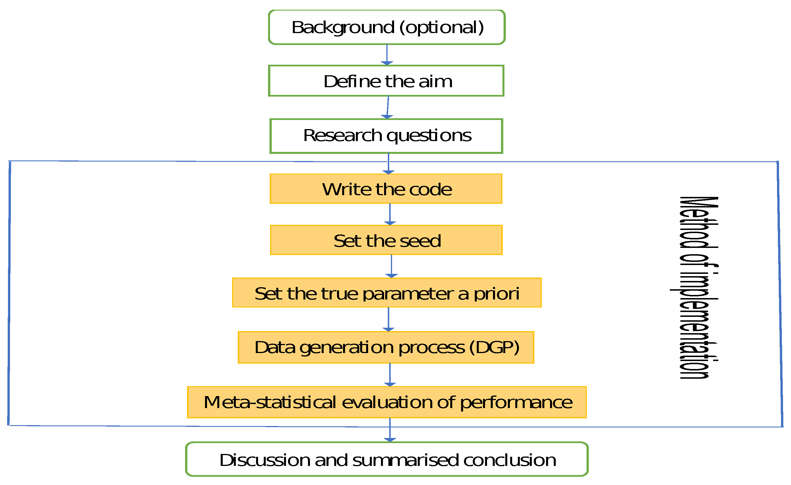
Figure 2.
QQ plots of = {10.3, 8.2, 4.1}.
Figure 3.
Time-varying location (top panel), scale (middle panel) and shape (bottom panel) parameters.
Figure 3.
Time-varying location (top panel), scale (middle panel) and shape (bottom panel) parameters.
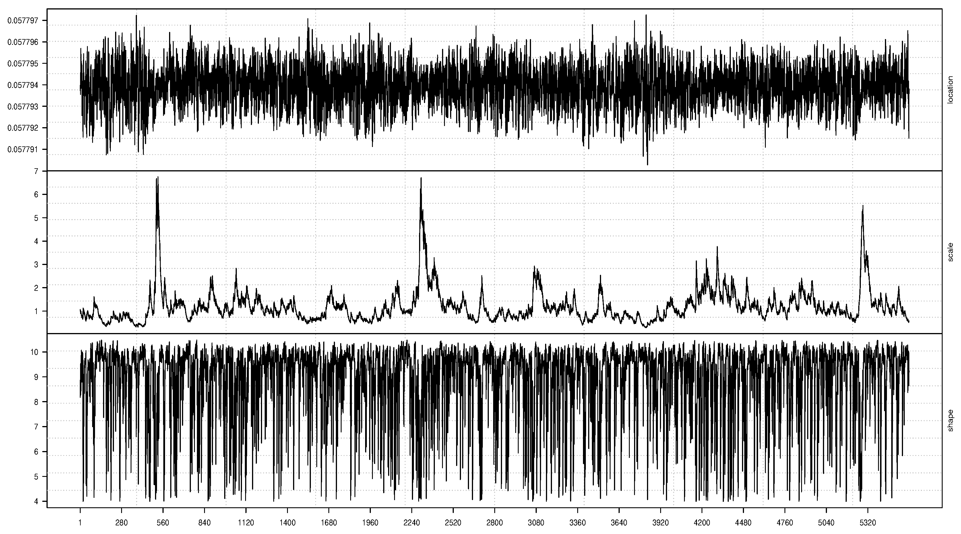
Figure 4.
The true parameter recovery (TPR) outlook. The dotted line is the 95% (i.e., 0.95) nominal recovery level.
Figure 4.
The true parameter recovery (TPR) outlook. The dotted line is the 95% (i.e., 0.95) nominal recovery level.
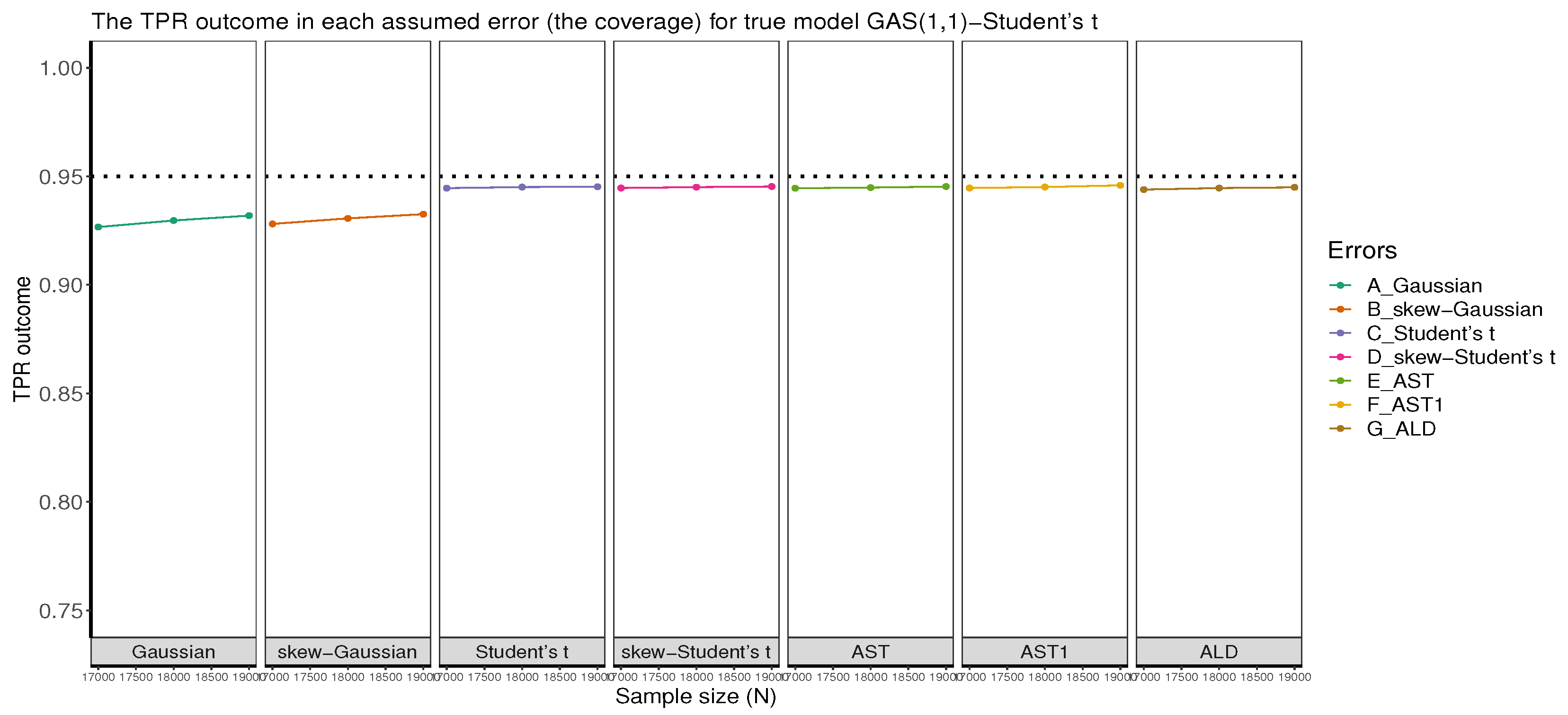
Figure 5.
AST1: Time-varying location (top panel), scale (upper-middle panel), skewness (lower-middle panel) and shape (bottom panel) parameters.
Figure 5.
AST1: Time-varying location (top panel), scale (upper-middle panel), skewness (lower-middle panel) and shape (bottom panel) parameters.
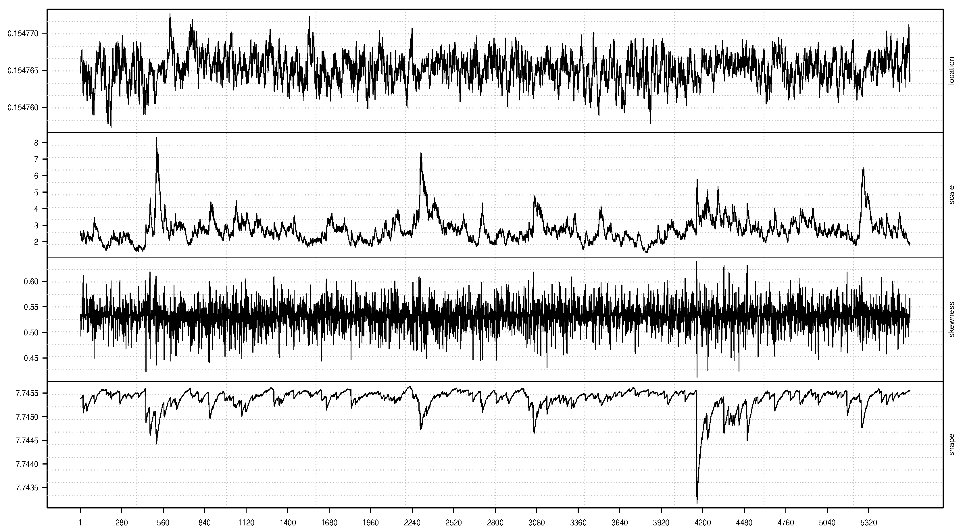
Figure 6.
The true parameter recovery (TPR) outlook. The dotted line is the 95% (i.e., 0.95) nominal recovery level.
Figure 6.
The true parameter recovery (TPR) outlook. The dotted line is the 95% (i.e., 0.95) nominal recovery level.
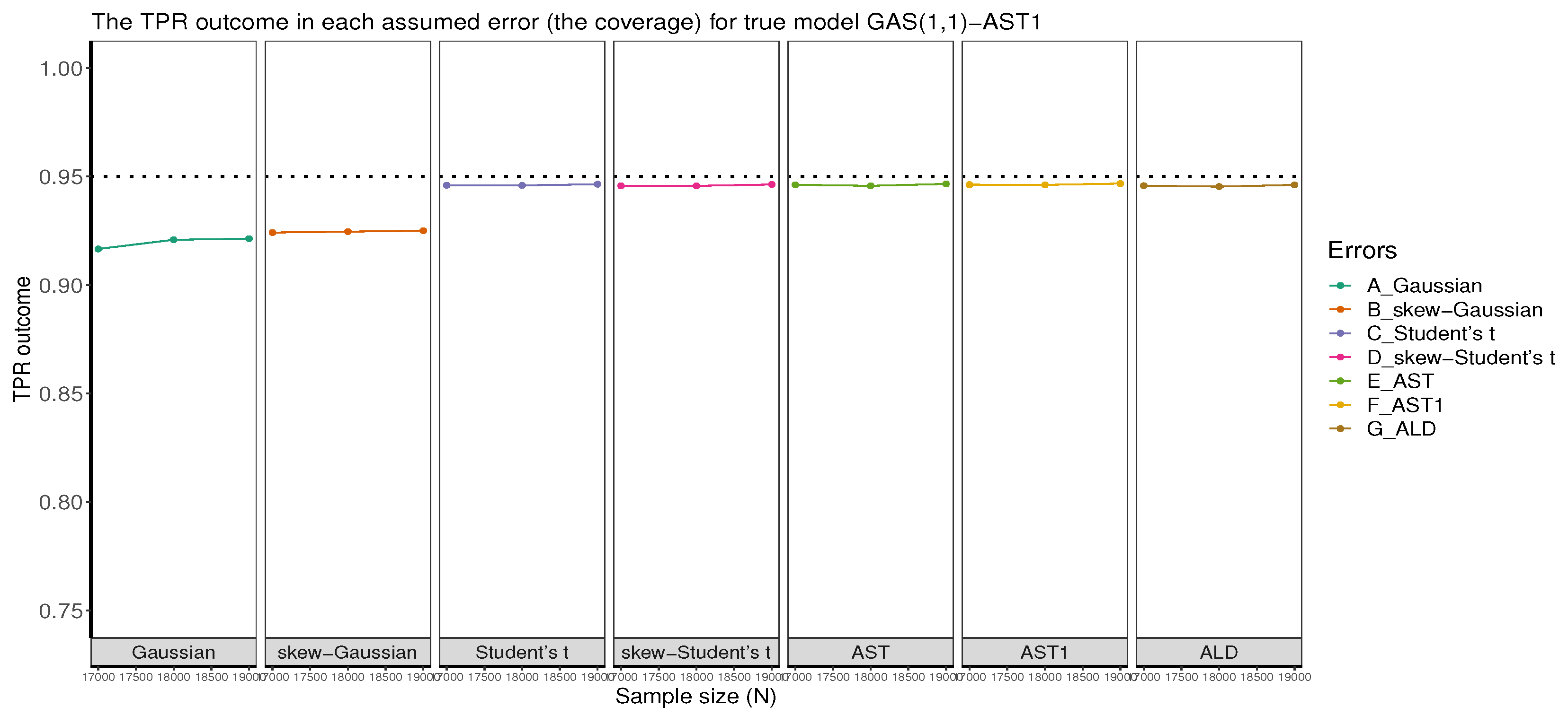
Figure 7.
Histograms of price (in Panel A) and returns (Panel B). The two colours merely demarcate the distribution where the price < 200 (with blue colour) and above 200 (with an indianred colour). This is also used where the returns < 0.
Figure 7.
Histograms of price (in Panel A) and returns (Panel B). The two colours merely demarcate the distribution where the price < 200 (with blue colour) and above 200 (with an indianred colour). This is also used where the returns < 0.
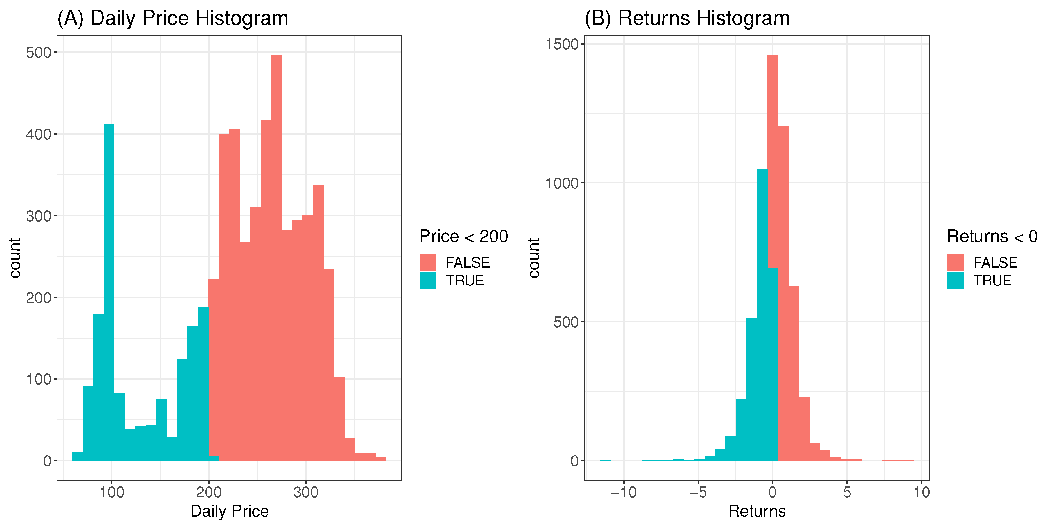
Figure 8.
Distributions of price (in Panel A) and returns (Panel B).
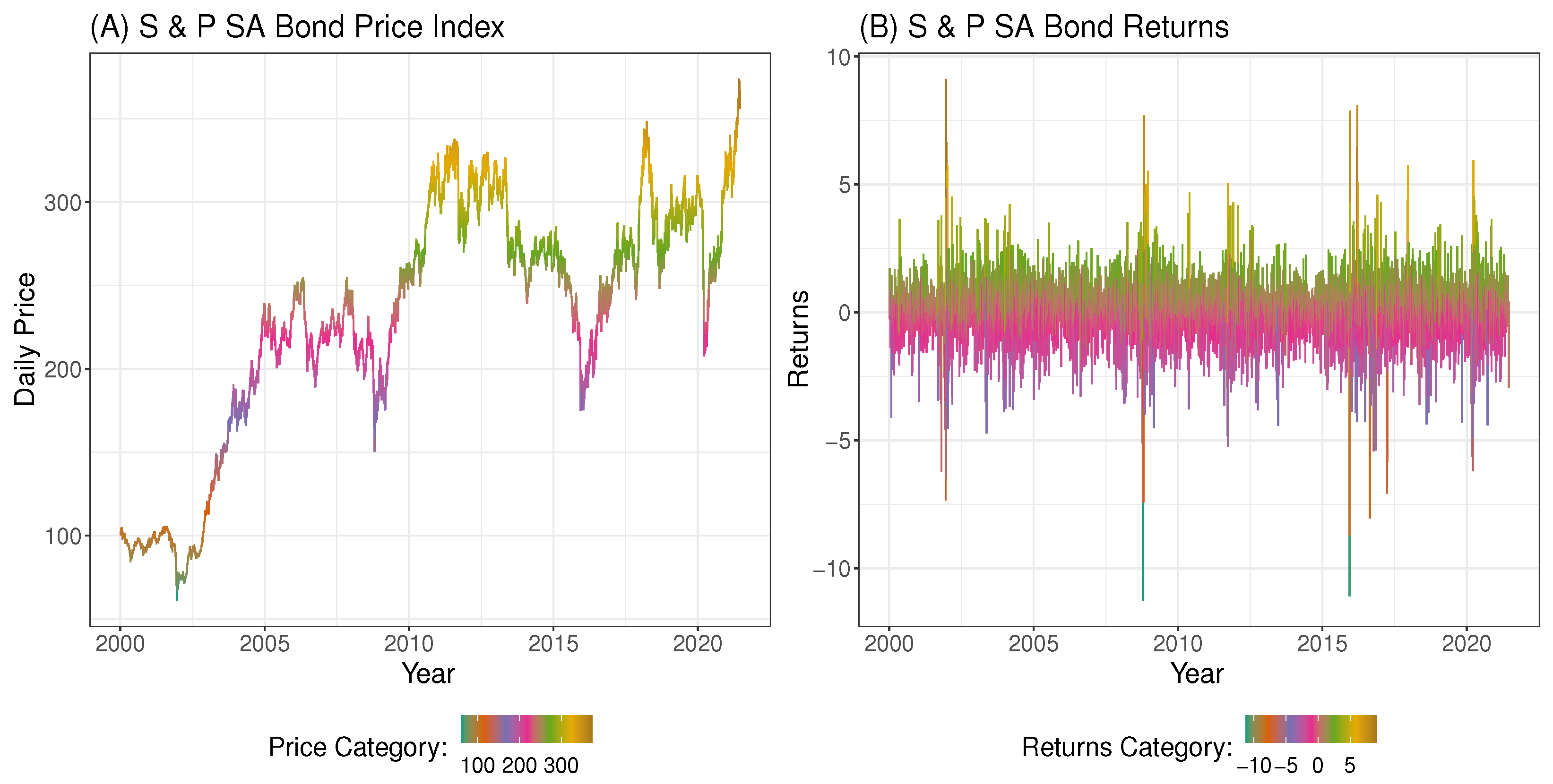
Figure 9.
Price and return densities in Panels A and B respectively, while Panels C and D display the price and return distributions with their densities.
Figure 9.
Price and return densities in Panels A and B respectively, while Panels C and D display the price and return distributions with their densities.
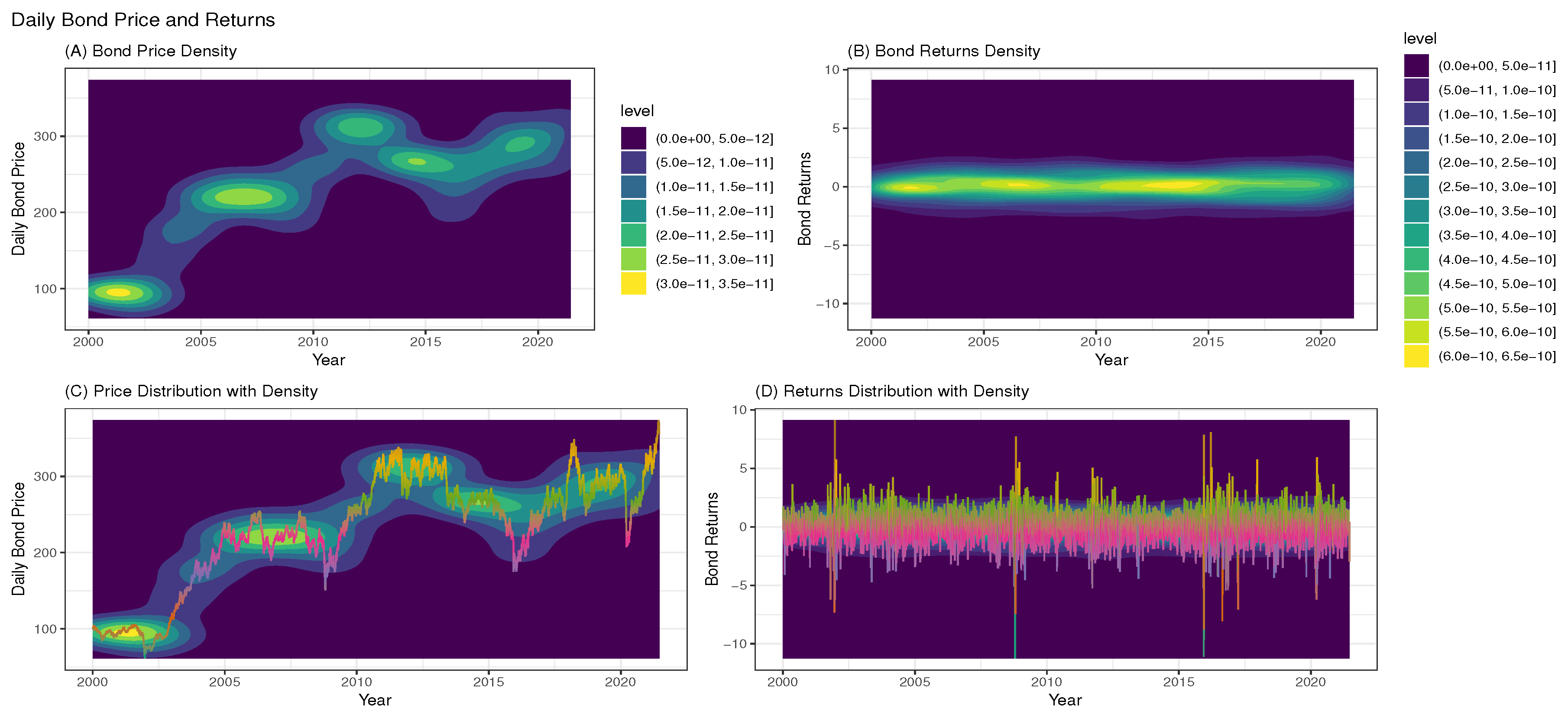
Figure 10.
Outcomes of serial correlation test.
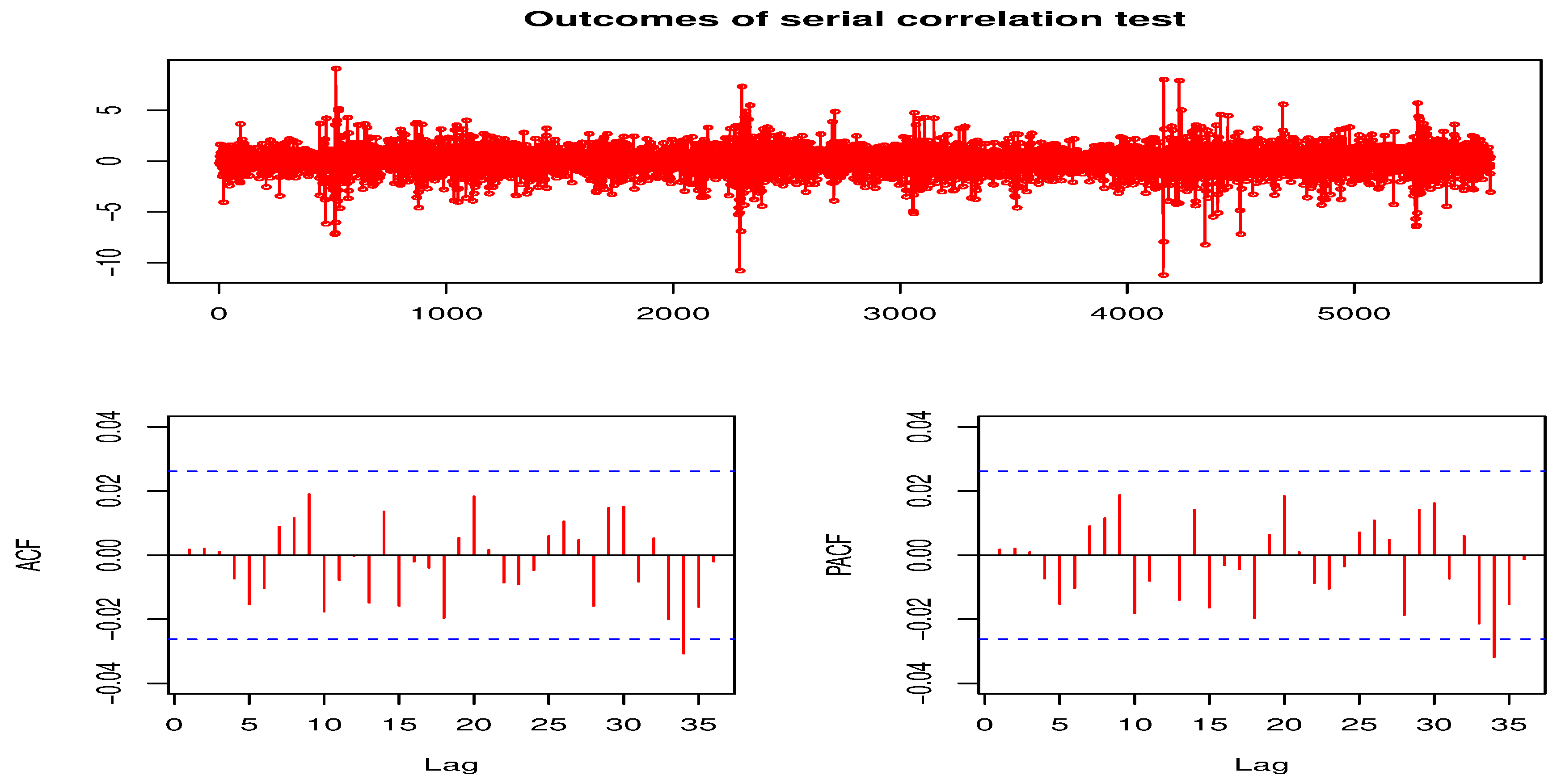

Table 1.
Simulation outcomes.
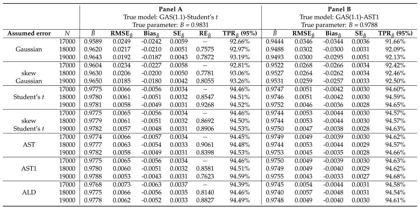 |
Table 2.
ARMA(1,1) and ARMA(2,2) models’ outcomes on Bond returns.
| ARMA(1,1) | ARMA(2,2) | |||||
| Normal | Student’s t | Normal | Student’s t | |||
| Test on standardized | WLB(9) | 2.2258 | 3.2100 | WLB(19) | 6.2949 | 10.3830 |
| residuals | p-value(9) | (0.9728) | (0.8563) | p-value(19) | (0.9573) | (0.4060) |
| Test on standardized | WLB(9) | 6.5740 | 7.4880 | WLB(19) | 6.4740 | 7.5450 |
| squared residuals | p-value(9) | (0.2376) | (0.1617) | p-value(19) | (0.2473) | (0.1577) |
Note: WLB denotes the Weighted Ljung-Box test, where "(9)" and "(19)" are lags 9 and 19, respectively.
Table 3.
Engle’s ARCH test results.
| ARMA(1,1) model | ARMA(2,2) model | |||||||
| PQ test | LM test | PQ test | LM test | |||||
| Lag order | PQ | P-value | LM | P-value | PQ | P-value | LM | P-value |
| 4 | 904 | 0 | 4729 | 0 | 888 | 0 | 4658 | 0 |
| 8 | 1127 | 0 | 2196 | 0 | 1104 | 0 | 2184 | 0 |
| 12 | 1400 | 0 | 1361 | 0 | 1377 | 0 | 1354 | 0 |
| 16 | 1517 | 0 | 1015 | 0 | 1497 | 0 | 1010 | 0 |
| 20 | 1575 | 0 | 807 | 0 | 1556 | 0 | 803 | 0 |
| 24 | 1624 | 0 | 666 | 0 | 1602 | 0 | 663 | 0 |
Note: PQ is the Portmanteau-Q statistic, and LM is the Lagrange-Multiplier statistic.
Table 4.
Empirical outcomes of GAS modelling on SA Bond return data.
| Normal | skew-Normal | Student t | skew-Student t | AST | AST1 | ALD | |
|---|---|---|---|---|---|---|---|
| 0.9804* | 0.9819* | 0.9790* | 0.9804* | 0.9788* | 0.9790* | 0.9784* | |
| AIC | 17936.36 | 17900.84 | 17682.49 | 17672.13 | 17668.28 | 17666.39 | 17910.63 |
| BIC | 17962.88 | 17933.99 | 17715.64 | 17711.91 | 17714.69 | 17706.17 | 17943.78 |
| Normal | skew-Normal | Student t | skew-Student t | AST | AST1 | ALD | |
| 0.9805* | 0.9819* | 0.9831* | 0.9818* | 0.9807* | 0.9818* | 0.9784* | |
| AIC | 17915.19 | 17904.84 | 17666.31 | 17672.84 | 17664.18 | 17650.89 | 17914.63 |
| BIC | 17954.97 | 17951.25 | 17725.98 | 17739.14 | 17737.11 | 17717.19 | 17961.04 |
Note: The "*" indicates 1% level of significance. Panel A shows the outcomes of the GAS fit for time-varying scale parameter, while Panel B gives the outcomes for time-varying location, scale, and shape parameters.
Disclaimer/Publisher’s Note: The statements, opinions and data contained in all publications are solely those of the individual author(s) and contributor(s) and not of MDPI and/or the editor(s). MDPI and/or the editor(s) disclaim responsibility for any injury to people or property resulting from any ideas, methods, instructions or products referred to in the content. |
© 2023 by the authors. Licensee MDPI, Basel, Switzerland. This article is an open access article distributed under the terms and conditions of the Creative Commons Attribution (CC BY) license (http://creativecommons.org/licenses/by/4.0/).
Copyright: This open access article is published under a Creative Commons CC BY 4.0 license, which permit the free download, distribution, and reuse, provided that the author and preprint are cited in any reuse.


