You are currently viewing a beta version of our website. If you spot anything unusual, kindly let us know.

Preprint

Article

Hyperparameter Optimization for Landslide Susceptibility Mapping: A Comparison between Baseline, Bayesian and Metaheuristic Hyperparameter Optimization Techniques for Machine Learning Algorithms

Altmetrics

Downloads

247

Views

140

Comments

A peer-reviewed article of this preprint also exists.

Farkhanda Abbas^*,

Feng Zhang,

Muhammad x Ismail,

Garee Khan,Javed Iqbal,

Abdulwahed F. Alrefaei

Mohammed Fahad Albeshr

Farkhanda Abbas^*,

Feng Zhang,

Muhammad x Ismail,

Garee Khan,Javed Iqbal,

Abdulwahed F. Alrefaei

Mohammed Fahad Albeshr

This version is not peer-reviewed

Abstract

Algorithms for machine learning have found extensive use in numerous fields and applications. One important aspect of effectively utilizing these algorithms is tuning the hyperparameters to match the specific task at hand. The selection and configuration of hyperparameters directly impact the performance of machine learning models. Achieving optimal hyperparameter settings often requires a deep understanding of the underlying models and the appropriate optimization techniques. While there are many automatic optimization techniques available, each with its own advantages and disadvantages, this article focuses on hyperparameter optimization for well-known machine learning models. It explores cutting-edge optimization methods and provides guidance on applying them to different machine learning algorithms. The article also presents real-world applications of hyperparameter optimization by conducting tests on spatial data collections for landslide susceptibility mapping. Based on the experiment's results, both Bayesian optimization and metaheuristic algorithms showed promising performance compared to baseline algorithms. For example, the metaheuristic algorithm improved the overall accuracy of the random forest model. Additionally, Bayesian algorithms, such as Gaussian processes, performed well for models like KNN and SVM. The paper thoroughly discusses the reasons behind the efficiency of these algorithms. By successfully identifying appropriate hyperparameter configurations, this research paper aims to assist researchers, spatial data analysts, and industrial users in developing machine learning models more effectively. The findings and insights provided in this paper can contribute to enhancing the performance and applicability of machine learning algorithms in various domains.

Keywords:

Subject: Computer Science and Mathematics - Computer Science

1. Introduction

Multiple fields of application, such as visual computing, language comprehension, suggestion engines, consumer activity analysis, and marketing have widely applied machine learning (ML) algorithms on a massive scale [1]. This is owing to the reality that they are versatile and proficient at solving data diagnosing issues. Different ML algorithms are appropriate for diverse varieties of datasets and issues [2]. Overall, developing competent ML models necessitates efficient fine-tuning of hyper-parameters based on the specifications of the chosen model [3].

Several alternatives must be examined to design and implement the most efficient ML model. Hyper-parameter optimization is the method of crafting an ideal model architecture using the optimal hyper-parameter configuration. The process of refining hyper-parameters is deemed crucial in generating a thriving machine learning model, specifically for deep neural networks and tree-based ML models, which contains an abundance of hyper-parameters. The hyper-parameter optimization process differs across ML algorithms due to the varied kinds of hyperparameters they employ, such as discrete, categorical, and continuous hyperparameters [4]. Non automatic traditional manual testing approach for hyper-parameter tuning is still widely used by advance degree research students, despite the requirement for a thorough comprehension of ML algorithms and the importance of their hyperparameter configurations [5]. Nevertheless, because of various factors, including complex models, numerous hyper-parameters, lengthy assessments, and non-linear hyper-parameter relationships, manual tuning is not effective for several reasons. These factors have spurred additional research on techniques for automatic hyper-parameter optimization, known as "hyper-parameter optimization" (HPO) [6].

The principal objective of Hyper-Parameter Optimization (HPO) is to streamline the hyper-parameter tuning system and empower users to effectively implement machine learning models to address real-world problems [3]. Upon completion of an HPO procedure, one expects to obtain the optimal architecture for an ML model. Below are some noteworthy justifications for utilizing HPO techniques with ML models:

Like numerous ML programmers devote significant time to adjusting the hyperparameters, notably for huge datasets or intricate ML algorithms having numerous hyperparameters, it decreases the degree of human labor required.
It boosts the efficacy of ML models. Numerous ML hyperparameters have diverse optimal values to attain the best results on different datasets or problems.
It boosts the replicability of the frameworks and techniques. Several ML algorithms may solely be justly assessed when the identical degree of hyper-parameter adjustment is applied; consequently, utilizing the equivalent HPO approach to several ML algorithms also assists in recognizing the ideal ML model for a specific problem.

To identify the most appropriate hyper-parameters, selecting the appropriate optimization technique is necessary. As a considerable number of HPO problems are complex nonlinear optimization challenges, they might not lead to a global optimum but rather to a local one. Therefore, standard optimization methods possibly inappropriate for HPO issues [7]. For continuous hyperparameters, the gradients can be computed by means of gradient descent-based techniques, which are a typical variant of conventional optimization algorithms [8]. As an example, a gradient-based method may be employed to enhance the learning rate in a neural network.

Numerous other enhancement methods, like decision-theoretic techniques, Multi fidelity optimization methods and Bayesian optimization models, and metaheuristic algorithms, are better suited for HPO challenges in contrast to traditional optimization techniques like gradient descent [4]. Several of these algorithms can precisely determine conditional, categorical, and discrete hyper-parameters as well as continuous hyper-parameters.

The methods based on decision theory are founded on the idea of constructing a search space for hyperparameters, identifying the hyperparameter combinations within the search space, and choosing the combination of hyperparameters with the highest performance. A decision-theoretic strategy called grid search (GS) [9] involves scanning through a predetermined range of hyperparameter values. Random search (RS) [10], another decision-theoretic approach, is used when execution time and resources are limited, and it randomly selects hyperparameter combinations from the search space. In GS and RS, each hyperparameter configuration is verified individually.

Bayesian optimization (BO) [11] models, in contrast to GS and RS, deduce the subsequent hyper-parameter value derived from the outcomes of the tried hyper-parameter values, avoiding several unnecessary assessments. Consequently, BO can recognize the optimal hyper-parameter fusion with lesser rounds of testing than GS and RS. BO can employ multiple models like the tree-structured Parzen estimators (TPE), the random forest (RF), and the Gaussian process (GP) [12]. As a surrogate function to model the distribution of the objective function for various scenarios. BO-RF and BO-TPE [12] can preserve the dependency of factors. Conditional hyper-parameters, such as the kernel type and A support vector machine’s (SVM) punishment parameter C, can be optimized using them. Parallelizing BO models is demanding because they function sequentially to strike a balance between discovering unexplored areas and exploiting regions that have already been tested.

Training an ML model often demands extensive labor and resources. To address resource constraints, multi-fidelity optimization algorithms, particularly those based on bandits, are widely used. A prevalent bandit-based optimization method called Hyperband [13] is an advanced version of RS. It produces downsized datasets and assigns an equal budget to every cluster of hyper-parameters. To save time and resources, Hyperband discards inferior hyper-parameter configurations in each cycle.

HPO problems are classified as intricate, non-linear, and extensive search space optimization problems, which are tackled utilizing metaheuristic algorithms [14]. The two most commonly employed metaheuristic algorithms for HPO are the Particle Swarm Optimization (PSO) and Genetic Algorithm (GA) [15,16]. In each iteration, genetic algorithms determine the most optimal hyper-parameter fusion and transmit those combinations to the ensuing iteration. In each cycle, every particle in PSO algorithms interacts with other elements to identify and revise the present global peak until it reaches the ultimate peak. Metaheuristics can efficiently explore the area and discover optimal or almost optimal solutions. Because of their superior efficiency, they are highly appropriate for HPO problems with extensive arrangement spaces.

Despite the fact that HPO algorithms are immensely useful in refining the effectiveness of ML models by adjusting the hyper-parameters, other factors, such as their computational intricacy, still have a lot of room for progress. However, as different HPO models have distinct advantages and limitations that make them suitable for addressing specific ML model types and issues, it is vital to take them all into account when selecting an optimization algorithm. This academic article provides the subsequent contributions:

It encompasses three well-known machine learning algorithms (SVM, RF and KNN) and their fundamental hyper-parameters.
It assesses conventional HPO methodologies, comprising their pros and cons, to facilitate their application to different ML models by selecting the fitting algorithm in pragmatic circumstances.
It investigates the impact of HPO techniques on the comprehensive precision of landslide susceptibility mapping.
It contrasts the increase in precision from the starting point and predetermined parameters to fine-tuned parameters and their impact on three renowned machine learning methods.

This overview article provides a comprehensive analysis of optimization approaches used for ML hyper-parameter adjustment issues. We specifically focus on the application of multiple optimization approaches to enhance model accuracy for landslide susceptibility mapping. Our discussion encompasses the essential hyper-parameters of well-known ML models that require optimization, and we delve into the fundamental principles of mathematical optimization and hyper-parameter optimization. Furthermore, we examine various advanced optimization techniques proposed for addressing HPO problems. Through evaluation, we assess the effectiveness of different HPO techniques and their suitability for ML algorithms such as SVM, KNN, and RF.

To demonstrate the practical implications, we present the outcomes of applying various HPO techniques to three machine learning algorithms. We thoroughly analyze these results and also provide experimental findings from the application of HPO on landslide dataset. This allows us to compare different HPO methods and explore their efficacy in realistic scenarios. In conclusion, this overview article provides valuable insights into the optimization of hyper-parameters in machine learning, offering guidance for researchers and practitioners in selecting appropriate optimization techniques and effectively applying them to enhance the performance of ML models in various applications.

Study Area

A region of roughly 332 km of the KKH expressway was analyzed. Conversely, the entire expanse of the route amounts to 1300 km, joining different provinces of Pakistan, like Punjab, Khyber Pakhtunkhwa, and Gilgit Baltistan with Xinjiang, an independent territory of China. The analysis was conducted in the north of Pakistan in the Gilgit, Hunza, and Nagar districts. There are various settlements along the KKH from Juglot, situated between 36°12′147″N latitude and 74°18′772″E longitude, moving through Jutal, Rahimbad, Aliabad, and culminating at Khunjarab Top, the China–Pakistan border crossing. The locality is positioned along the Indus River, Hunza River, and Gilgit River. The evaluated zone measures 332 km in length and 10 km in radius, covering 3320 km2 along the KKH. The majority of the area is hilly, with the highest peak reaching 5370 m and the lowest elevation being 1210 m. Snowslides, mudslides, and tremors are frequent natural hazards in this region. A rockslide or rubble fall set off by precipitation or seismic movements is the most prevalent type of landslide in our evaluation domain (Figure 1).

Landslide Conditioning Factors

Eight different landslide conditioning factors used in our case study are presented in Figure 2 and further details of these variables are mentioned in Table 1 below.

2. Methodology

As a starting point, the landslide dataset along KKH, which is a pure classification problem, serves as the gauge dataset for the examination of the HPO method on data analysis issue.

The subsequent step involves configuring the ML models with their objective function. Based on the characteristics of their hyper-parameters, all popular ML models are categorized into five groups explain in Section 3. The three most common examples of these ML categories are "one categorical hyper-parameter," "a few conditional hyper-parameters," and "a wide hyper-parameter configuration space with multiple categories of hyper-parameters. RF, KNN, and SVM are chosen as the three ML algorithms to be adjusted since their hyper-parameter types correspond to the three typical HPO scenarios: each sample’s closest neighbors in terms of KNN is a crucial hyper-parameter; the penalty parameter and the kernel type C are a few conditional hyper-parameters in SVM; As described in Section 6, RF has a number of many kinds of hyper-parameters. Additionally, KNN, SVM, and RF can solve classification problems.

The evaluation metric and evaluation technique are determined in the subsequent step. The HPO methods employed in our experiment on the chosen dataset are evaluated using 3-fold cross-validation. In our experiments, the two most common performance measurements are utilized. The accuracy, which is the ratio of precisely labeled data, is used as the classifier performance parameter for classification models, and the model efficiency is also calculated using the computational time (CT), which is the overall time required to complete an HPO procedure with threefold cross-validation.

Subsequently, a number of criteria must be met to accurately compare various optimization methods and frameworks. In order to compare different HPO techniques, we first utilize the same hyper-parameter configuration space. For each evaluation of an optimization approach, the single hyper-parameter for KNN, 'n neighbors,' is set to be in the similar span of 1 to 20. For each type of problem, the hyper-parameters for SVM and RF models for classification problems are also set to be in the same configuration space. Table 3 displays the characteristics of the setup space for ML models.

Drawing from the notions presented in Section 3 and manual experimentation, the selected hyper-parameters and their exploration domain are identified [120]. Table 2 likewise details the hyper-parameter categories for each ML technique.

Section 4 introduces six different hyperparameter optimization (HPO) approaches. To evaluate their performance, we chose six representative HPO methods discussed in Section 4, namely Grid Search (GS), Genetic Algorithm (GA), the Random Search (RS), the Bayesian Optimization with the Gaussian Process (BO-GP), and the Bayesian Optimization with the Tree-structured Parzen Estimator (BO-TPE), and Particle Swarm Optimization (PSO). To ensure unbiased empirical conditions for each HPO approach, the HPO experiments were carried out based on the procedures outlined in Section 2. Python 3.5 was used for all experiments, which were carried out on a system with a Core i7 processor and 32 GB of RAM. To investigate the associated machine learning and HPO methods, a variety of open-source Python modules and frameworks were used, encompassing sklearn [30], Skopt [110], Hyperopt [106], Optunity [79], Hyperband [16], BOHB [93], and TPOT [118].

3. Hyper-Parameters

Hyperparameter configuration characteristics can be used to categorize ML algorithms. Based on these features, suitable optimization methods can be selected to optimize the hyper-parameters.

3.1. Discrete Hyper-Parameter

Discrete hyperparameter typically needs to be modified for some ML algorithms, such as specific neighbor-based, clustering, and dimensionality reduction algorithms. The primary hyper-parameter for KNN is the number of considered neighbors, or k. The number of clusters is the most important hyper-parameter for k-means, hierarchical clustering, and EM. Similar to this, the fundamental hyper-parameter for dimensionality reduction techniques like PCA and LDA is "n components," or the quantity of features to be retrieved. The best option under these circumstances is Bayesian optimization, and the three surrogates might be evaluated to see which is most effective. Another excellent option is hyperband, which may have a quick execution time because of its parallelization capabilities. In some circumstances, users may want to fine-tune the ML model by taking into account other less significant hyper-parameters, such as the distance metric of KNN and the SVD solver type of PCA; in these circumstances, BO-TPE, GA, or PSO could be used.

3.2. Continuous Hyper-Parameter

several nave Bayes algorithms, such as multinomial NB, Bernoulli NB, and complement NB, as well as several ridge and lasso methods for linear models typically only have one crucial continuous hyper-parameter that needs to be set. The continuous hyper-parameter for the ridge and lasso algorithms is "alpha," or the regularization strength. The key hyper-parameter, commonly known as "alpha," in the three NB algorithms stated above really refers to the additive (Laplace/Lidstone) smoothing value. The best option among these ML algorithms is BO-GP since it excels at optimizing a constrained set of continuous hyper-parameters. Although gradient-based algorithms are also possible, they may only be able to find local optimum locations, making them less efficient than BO-GP.

3.3. Conditional Hyper-Parameters

It is apparent that many ML algorithms, including SVM, LR, and DBSCAN, have conditional hyper-parameters. 'penalty', 'C', and the solver type are the three correlated hyper-parameters of LR. Similar to DBSCAN, 'eps' and 'min samples' need to be tweaked together. SVM is more complicated because, after choosing a new kernel type, a unique set of conditional hyper-parameters must be calibrated. As a result, some HPO techniques, such as GS, RS, BO-GP, and Hyperband, which cannot successfully optimize conditional hyper-parameters, are not appropriate for ML models with conditional hyper-parameters. If the correlations between the hyper-parameters are known in advance, BO-TPE is the ideal option for these ML approaches. SMAC is an additional option that works well for fine-tuning conditional hyper-parameters. You can also utilize GA and PSO.

3.4. Categorical Hyper-Parameters

Given that their primary hyper-parameter is a categorical hyper-parameter, ensemble learning algorithms tend to use this category of hyper-parameters. The categorical hyper-parameter for bagging and AdaBoost is "base estimator," which is configured to be a single ML model. 'Estimators' is the term used for voting and denotes a list of ML single models that will be integrated. 'Voting' is a further categorical hyper-parameter of the voting method that is used to select between a hard and soft voting approach. To evaluate whether these categorical hyper-parameters are a viable base for machine learning, GS would be adequate. However, other hyper-parameters, such as 'n estimators', 'max samples', and 'max features' in bagging, as well as 'n estimators' and 'learning rate' in AdaBoost, frequently need to be taken into account; as a result, BO algorithms would be a better option to optimize these continuous or discrete hyper-parameters. In conclusion, the most appropriate HPO method should be chosen based on the characteristics of its hyper-parameters when adjusting an ML model to obtain high model performance and low computing costs.

3.5. Big Hyper-Parameter Configuration Space with Different Types of Hyper-Parameters

Since they have numerous hyper-parameters of diverse, different types, tree-based algorithms in ML, such as DT, RF, ET, and XGBoost, as well as DL algorithms, such as DNN, CNN, and RNN, are the most difficult to fine-tune. PSO is the ideal option for these ML models since it allows for parallel executions to increase efficiency, especially for DL models that frequently require a significant amount of training time. Other techniques like GA, BO-TPE, and SMAC can also be utilized, however they might take longer than PSO to complete because it is challenging to parallelize these approaches.

4. Hyper-Parameter Optimization Techniques:

4.1. Babysitting

A primary method for adjusting hyper-parameters is babysitting, often referred to as "Trial and Error" or graduate student descent (GSD) [5]. Pupils and intellectuals equally frequently utilize this completely hands-on adjustment technique. The procedure is simple: following the creation of a machine learning (ML) prototype, the student experiments with a range of potential hyper-parameter values founded on knowledge, speculation, or examination of outcomes from prior evaluations. This procedure is reiterated until the student exhausts the time limit (often meeting a deadline) or is content with the outcomes. Consequently, this technique necessitate sufficient background knowledge and expertise to quickly find the optimal hyper-parameter values. Because of various reasons, including numerous hyper-parameters, intricate models, time-consuming prototype evaluations, and nonlinear hyper-parameter interactions, manual adjustment is often unfeasible [6]. These concerns prompted further research into methods for self-regulating hyper-parameter optimization [17].

4.2. Grid Search

frequently utilized methods for exploring the hyper-parameter configuration space is grid search (GS) [2]. GS can be seen as a brute-force approach that analyzes every feasible permutation of hyper-parameters that is given, to the matrix of configurations. When a user-defined bounded range of values is utilized, GS assesses the cross product of those values [7].

GS is incapable of completely employing the fruitful zones alone. To discover the global maximum, the subsequent procedure needs to be executed manually [2]:

Commence with a wide exploration region and sizable stride length.
Utilizing prior effective hyper-parameter settings, diminish the exploration area and stride length.
Persist in repeating step 2 until the optimum outcome is achieved.

Grid search (GS) is easy to parallelize and deploy. Nonetheless, its primary drawback is that it becomes inefficient for hyper-parameter configuration spaces with a high number of dimensions since it necessitates exponentially more evaluations as the number of hyper-parameters increases. This exponential increase is known as the "curse of dimensionality" [18]. If GS involves k variables, and each one has n unique values, then the computational intricacy of GS grows exponentially at a rate of

O (n^{k})

[16]. Consequently, GS can only serve as a practical HPO method when the hyper-parameter search space is limited.

4.3. Random Search

to surmount some of the limitations of grid search (GS), random search (RS) was introduced in [10] RS, similar to GS, selects a specific sample quantity, from the search space within upper and lower thresholds as potential hyper-parameter values at random, train these possibilities, and iterates the process until the cost limit is depleted. The RS hypothesis suggests that the global optima, or at least their close values, can be uncovered if the configuration space is sufficiently extensive. in spite of possessing a limited budget, RS is capable of exploring more terrain than GS [10].

Due to its autonomous nature, one of the fundamental benefit of Random Search (RS) is that it can be easily parallelized and resource allocation can be managed efficiently. Unlike Grid Search (GS), RS chooses a fixed number of parameter variations from the provided distribution, thereby increasing the operational efficiency by reducing the likelihood of idle periods on a small, insignificant search space.

The computational intricacy of Random Search (RS) is O(n) as the total number of assessments in RS is predetermined to be n prior to the optimization commences [19]. Additionally, with enough h resources, RS can determine the global optimum or the nearly optimal solution [20].

Random search (RS) is more efficient than grid search (GS) for extensive search areas. However, because it disregards previously successful regions, there are still a significant number of unnecessary function evaluations [2].

Consequently, both RS and GS waste substantial amounts of time evaluating areas of the search space that perform poorly, as each iteration's review is independent of prior evaluations. Other optimization methods, such as Bayesian optimization, which rely on information from past evaluations to guide subsequent evaluations, can overcome this issue [11].

Bayesian Optimization

Iterative Bayesian optimization (BO) is a common approach to solving HPO problems [21]. contrasting GS and RS, BO uses past results to determine future evaluation points. BO employs two essential, elements, a surrogate model and an acquisition function, to define the next hyper-parameter configuration [22].

All sample points are aimed to correspond to the surrogate model for the objective function. The optimization function utilized the stochastic surrogate model's prediction distribution to weigh the compromise between searching and manipulation and identify which points to use. Exploitation involves sampling in present areas where, according to the posterior distribution, the global optimum is most likely to occur, whereas exploration entails sampling in uncharted territory. BO models integrate the exploration and exploitation procedures to determine the best places and avoid missing improved configurations in uncharted territory [23].

The following are the essential stages of Bayesian optimization (BO) [11]:

Create a surrogate probabilistic model of the target function.
Find the best hyper-parameter values on the surrogate model.
Employ these hyper-parameter values to the existing target function for evaluation.
Add the most recent observations to the surrogate model.
Repeat steps 2 through 4 until the allotted number of iterative cycles is reached.

Therefore, BO operates by revising the surrogate model after each assessment of the target function. Because it can identify the optimal hyper-parameter combinations by evaluating the results of prior tests and because operating a surrogate model is commonly much less expensive than running actual target function, BO is more effective than grid search (GS) and random search (RS).

Although Bayesian optimization models are sequential techniques that are hard to parallelize, they can frequently identify nearly optimal hyper-parameter combinations in a limited number of iterations [4].

Tree Parzen estimator (TPE), Gaussian process (GP), and random forest (RF) are commonly used surrogate models for BO. Derived from their surrogate models, the three primary categories of BO algorithms are BO-GP, BO-RF, and BO-TPE. In our study on landslide data, we used BO-GP and BO-TPE. Sequential model-based algorithm configuration (SMAC) is another name for BO-RF [24].

4.4. BO-GP

The Gaussian process (GP) is a widely used alternative model for objective function modeling in Bayesian optimization (BO) [21]. The predictions follow a normal distribution when the function f is a realization of a GP with a mean

μ

and a covariance

σ^{2}

[25]:

p (y| x, D) = N (y| \hat{μ}, {\hat{α}}^{2}),

(1)

Let D denote the hyper-parameter configuration space, where y = f(x) represents the outcome analysis for every hyper-parameter x. Subsequent evaluation points are chosen from the precise bounds created by the BO-GP model after making predictions. The sample records are revised with every new data point tested, and the BO-GP model is reconstructed using the revised data. This process is iterated until completion.

BO-GP's application to a dataset of size n has a time and space complexity of

O (n^{3})

and

{O (n}^{2})

respectively [26]. The limitation of the number of instances to cubic complexity hinders its ability to be parallelized, which is a major disadvantage of BO-GP [3]. Moreover, it is mainly utilized for optimizing continuous variables.

4.5. BO-TPE

An alternative common surrogate model for Bayesian optimization (BO) is the TPE, a Parzen estimator based on a tree structure [9]. Instead of using the predictive distribution employed in BOGP [3], BO-TPE constructs two solidity functions, namely

l (x)

and

g (x)

, to act as generative models for entire variable range. The recorded results are divided into favorable and unfavorable outcomes based on a pre-defined percentile value

y^{*}

, and TPE is applied by utilizing simple Parzen windows [9] to model each group of results:

p (x| y, D) = \{\begin{matrix} l (x), i f y < y^{*} \\ g (x), i f y > y^{*} \end{matrix}

(2)

The proportion between the two solidity functions is subsequently used to establish the fresh setups for assessment, mirroring the predicted enhancement in the acquisition function. The provided contingent interdependencies are conserved as the Parzen estimators are organized in a hierarchical format. Consequently, TPE inherently facilitates conditional hyperparameters [25]. BO-TPE has a lower time complexity of

O (n l o g n)

[3] compared to BO-GP.

BO techniques work well for many HPO issues, regardless of how uncertain, non-linear, or non-smooth the objective function f is. If BO models don't strike a balance between exploitation and exploration, they may only reach a local rather than a global optimum. RS is not limited by this disadvantage as it lacks a specific focus area. Additionally, BO approaches are difficult to parallelize as their intermediate results are interdependent [4].

4.6. Metaheuristic Algorithms

A category of algorithms recognized as metaheuristic algorithms [26] are often utilized for optimization problems. They are mainly stimulated by biological concepts. Metaheuristics can effectively address optimization problems that are not convex, not smooth, or not continuous, divergent from several traditional optimization methods. One of the primary classifications of metaheuristic algorithms is population-based optimization algorithms (POAs), that also involve evolutionary algorithms, genetic algorithms (GAs), particle swarm optimization (PSO), and evolutionary strategies. Each generation in POAs commences with the formation and modernization of a community, afterward each person is evaluated until the global best is found [11]. The methods employed to form and choose populations are the fundamental differences among diverse POAs [14]. Since given population of N individuals can be assessed on utmost N threads or processors concurrently, POAs are effortless to parallelize [20]. The two most commonly utilized POAs for HPO problems are particle swarm optimization and genetic algorithms.

4.7. Genetic Algorithm (GA)

Among the well-liked metaheuristic algorithms, the genetic algorithm (GA) [15] is grounded on the evolutionary concept that individuals with the best survival and environmental adaptability are more prone to endure and transfer those abilities to future generations. The ensuing generation might comprise of both superior and inferior individuals, and they will also inherit the characteristics of their forebears. Superior individuals will have a higher chance of surviving and producing competent progeny, while the inferior individuals will gradually vanish from the population. The individual who is most adaptable will be acknowledged as the global optimum after several successions [27].

Each chromosome or individual functions as a hyper-parameter when utilizing GA to HPO problems, and its decimal value functions as the hyper-parameter's genuine input value in each assessment. Each chromosome has a variety of genes, which are portrayed by binary digits. The genes on this precise chromosome are consequently subjected to crossover and mutation procedures. The population is comprised of all values inside the initialized chromosome/parameter ranges, and the fitness function specifies the metrics used to evaluate the parameters [27].

As the optimal parameter values are often missing from the randomly-initialized parameter values, it is crucial to perform multiple actions on the well-adapted chromosomes, involving crossover, selection, and mutation methods, to discover the best values [15]. Chromosome picking is performed by selecting those with high values in the fitness function. The chromosomes that have high fitness function values are predisposed to be inherited by the next generation, so they create new chromosomes with the superior attributes of their parents, in order to maintain a constant population size. Chromosome selection allows positive traits from one generation to be passed on to the following successions. Crossover is utilized to produce new chromosomes by transferring a segment of genes from various chromosomes. Mutation techniques can also be utilized to produce new chromosomes by randomly altering one or more chromosome genes. Techniques such as mutation and crossover promote diverse traits in later generations and decrease the chances of missing desirable traits [3].

The following are the primary GA procedures [26]:

Commence by randomly initializing the genes, chromosomes, and population that depict the whole exploration space, as well as the hyper-parameters and their corresponding values.
Identify the fitness function, which embodies the main objective of an ML model, and employ the findings to evaluate each member of the current generation.
Use chromosome methodologies such as crossover, mutation, and selection to generate a new generation comprising the subsequent hyper-parameter values that will be evaluated.
Continue executing steps 2 and 3 until the termination criteria are met.
Conclude the process and output the optimal hyper-parameter configuration.

Amidst the previously mentioned procedures, the population initiation phase is critical for both PSO and GA because it offers an initial approximation of the ideal values. A proficient population initiation approach can significantly accelerate convergence and enhance the effectiveness of POAs, despite the fact that the initiated values will be progressively enhanced throughout the optimization process. An appropriate starting population of hyperparameters ought not to be restricted to an unfavorable area of the exploration space and instead, should include individuals in proximity to global optima by considering the encouraging domains [28].

In GA, random initiation, which merely generates the initial population with arbitrary values within the specified exploration space, is frequently utilized to produce hyperparameter configuration potential for initial population [29]. As a result of its selection, crossover, and mutation operations, GA is uncomplicated to construct and does not necessitate exceptional initializations. This reduces the probability of losing out the global optimum.

Consequently, it is beneficial to determine a probable acceptable initial exploration space for the hyperparameters when the data analyst has limited expertise. The primary disadvantage of GA is that the approach introduces novel hyperparameters that must be specified, such as the population magnitude, fitness function kind, crossover percentage, and mutation percentage. Additionally, GA is a successive execution method, making parallelization difficult. GA has an

O (n^{2})

time complexity [30]. GA may occasionally prove ineffective due to its slow convergence pace.

4.8. Particle Swarm Optimization (PSO)

A different group of evolutionary algorithms often utilized for optimization problems is the particle swarm optimization (PSO) [31]. PSO algorithms take inspiration from biological communities that demonstrate both individual and cooperative inclinations [14]. PSO functions by enabling a cluster of particles to navigate the exploration area in a partially random manner [6]. Through teamwork and exchange of knowledge among the particles within the cluster, PSO algorithms determine the optimal solution.

Collection S of n particles is present in PSO as [2]:

s = (s_{1}, s_{2}, \dots \dots \dots, s_{n}),

(3)

and every particle

S_{i}

is expressed by a vector:

S_{i} = < \vec{x_{i}}, \vec{v_{i}}, \vec{p_{i}} >,

where

\vec{x_{i}}

represent the current location,

\vec{v_{i}}

represent the current speed, and

\vec{p_{i}}

is the best position of the swarm up until the current iteration.

Initially, every particle is generated randomly in terms of position and speed using PSO. Every particle then analyze its current location and stores it along with its performance grades. In the subsequent iterations, the velocity of each particle

\vec{v_{i}}

is updated rooted on its most recent global best position

\vec{p}

and its previous position

\vec{p_{i}}

\vec{v_{i}} ≔ \vec{v_{i}} + U (0, φ_{1}) (\vec{p_{i}} - \vec{x_{i}}) + U (0, φ_{2}) (\vec{p} - \vec{x_{i}}),

(4)

where the acceleration constants

φ_{1}

and

φ_{2}

are used to calculate the continuous uniform distributions

U (0, φ)

The particles then travel according to their new velocity vectors:

\vec{x_{i}} ≔ \vec{x_{i}} + \vec{v_{i}}

The above steps are iterated until the termination criteria are met in PSO. Contrasted to GA, PSO is simpler to execute because it doesn’t require incremental steps like crossover and mutation. In GA, all chromosomes interact with each other, resulting in the entire population moving towards the optimal region uniformly. In contrast, PSO only shares knowledge on top individual particles and the global superior particles, resulting in a unidirectional transmission of information and the search process moving towards the current optimal solution [2]. The computational complexity of the PSO algorithm is

O (nlog n)

[32], and its convergence rate is generally faster than that of GA. Moreover, PSO particles function autonomously and solely required to exchange information with each other after each iteration, making it easy to parallelize the process and increase model efficiency [6].

The primary deficiency of PSO is that it may solely attain a local rather than a global optimum, particularly for discrete hyper-parameters, in the absence of appropriate population initialization [33]. Adequate population initialization can be achieved by developers with previous experience or population initialization methods. Multiple strategies for population inception, such as the opposition-based optimization algorithm [29] and the space transformation search approach [34], have been devised to enhance the performance of evolutionary algorithms. Additional population inception methods will require more resources and execution time.

Hyperparameter configuration characteristics can be used to categorize ML algorithms. Based on these features, suitable optimization methods can be selected to optimize the hyper-parameters.

5. Mathematical and Hyper-Parameter Optimization

Machine learning is primarily used to address issues with efficiency. To accomplish this, a weight parameter improvement technique for an ML model is used until the objective function value reaches a minimum value and the accuracy rate reaches a maximum value. Similar to this, methods for optimizing hyperparameter configurations aim to improve a machine learning model's architecture. The fundamental ideas of mathematical optimization are covered in this part, along with hyperparameter optimization for machine learning models.

5.1. Mathematical Optimization

The aim of mathematical optimization is to locate the optimal solution from a pool of possibilities that maximized or minimized objective function [35]. Depending on whether restrictions are placed on the choice or the solution variables, optimization problems can be classified as either constrained or unconstrained. A decision variable x in unconstrained optimization problems can take on any value from the one-dimensional space of real numbers, R. This problem is an unconstrained optimization problem [36].

\min_{x \in R} f (x)

(1)

where the goal function is f(x).

In contrast, constrained optimization problems are more prevalent in real-world optimization problems. The decision variable x in constrained optimization problems, must satisfy specific constraints, which can be equalities or inequalities in mathematics. Therefore, optimization problems can be expressed as general optimization problems or constrained optimization problems [36].

\begin{matrix} \min_{x} f (x) \\ Subject to \\ g_{i} (x) \leq 0, i = 1,2, \dots \dots \dots \dots, m, \\ h_{j} (x) = 0, j = 1,2, \dots \dots \dots \dots, p, \\ x ϵ X, \end{matrix}

(2)

where X is the domain of x,

g_{i} (x) \leq 0, i = 1,2, \dots \dots \dots \dots, m,

are the inequality constraint functions, and

h_{j} (x) = 0, j = 1,2, \dots \dots \dots \dots, p,

are the equality constraint functions.

Constraints serve the purpose of limiting the feasible region, or the possible values of the optimal answer, to specific regions of the search space.

As a result, the feasible area D of x can be illustrated as follows:

D = \{x \in X| g_{i} (x) \leq 0, h_{j} (x) = 0\} .

(3)

An objective function f(x) that can be minimized or maximized, a collection of decision variables x, and an optimization problem are the three main components. The variables may be allowed to take on values within a certain range by a set of constraints that apply to the issue. if the optimization issue is constrained. Determining the collection of variable values that minimizes or maximizes the objective function while satisfying any necessary constraints is the aim of optimization problems.

The viable range of the cluster count in k-means, as well as temporal and spatial limitations, are typical constraints in HPO problems. Consequently, constrained optimization methods are frequently employed in HPO problems.

In many situations, optimization problems may converge to a local optima rather than a global optimum. For example, when seeking the minimum value of a problem, suppose that D is the viable region of a decision factor x. A global minimum is the point

x^{*} \in D

satisfy

f (x^{*}) \leq f (x) \forall x \in D

, whereas a local minimum is the point

x^{*} \in D

in a vicinity N satisfy

f (x^{*}) \leq f (x) \forall x \in N \cap D

[36]. As a result, the local optimum only exists in a limited range and might not be the best option for the full possible region.

Only convex functions have the guarantee that a local optimum is also the global optimum [37]. Convex functions are those that have a single optimum. Consequently, the global optimal value can be found by extending the search along the direction in which the objective function declines.

f(x) is a convex function if and only if [37], for

\forall x_{1}, x_{2} \in X, \forall t \in [0,1],

f (t x_{1} + (1 - t) x_{2}) \leq f (x_{1}) + (1 - t) f (x_{2}),

(4)

where t is a coefficient with a range of [0,1] and X is the domain of the choice variables. Only when the viable region C is a convex set and the objective function f(x) is a convex function is an optimization issue a convex optimization problem [37].

\min_{x} f (x)

(5)

Subject to

x \in

Conversely, nonconvex functions only have one global optimum while having several local optimums. Nonconvex optimization problems make up the majority of ML and HPO issues. Inappropriate optimization techniques frequently only find local rather than global optimums.

Traditional techniques such as Newton's method, conjugate gradient, gradient descent, and heuristic optimization techniques can all be utilized to address optimization problems [35].Gradient descent is a popular optimization technique that moves in the opposite direction of the positive gradient as the search trajectory as it approaches the optima. The global optimum, however, cannot be detected with certainty via gradient descent unless the objective function is convex. The Hessian matrix's inverse matrix is used by Newton's technique to determine the optimal solution. Despite needing more time and space to store and construct the Hessian matrix than gradient descent, Newton's approach offers a faster convergence speed.

To find the best solution, conjugate gradient searches are conducted across conjugated direction created by the gradient of known data samples. Conjugate gradient has a higher rate of convergence than gradient descent, but its computation is more difficult. Heuristic methods, in contrast to other conventional approaches, solve optimization issues by applying empirical rules rather than by following a set of predetermined processes to arrive at the solution. Heuristic techniques frequently find the estimated global optima after a few rounds, although they can’t always find the global optimum [35].

5.2. Hyper-Parameter Optimization

Throughout the ML model design phase, the optimal hyper-parameters can be identified by efficiently exploring the hyperparameter space using optimization techniques. The hyper-parameter optimization procedure comprises four key constituent: an estimator also known as a regressor or classifier with a goal function, a search space or configuration space, an optimization or search method to find combinations of hyper-parameters, and an evaluation function to gauge how well different hyper-parameter configurations work.

Hyper-parameters, like whether to employ early halting or the learning rate, can have categorical, binary, discrete, continuous, or mixed domains. Thus, categorical, continuous, and discrete hyper-parameters are the three categories of hyper-parameters. The domains of continuous and discrete hyper-parameters are often restricted in real-world applications. Hyper-parameter configuration spaces can also include conditional hyper-parameters, which must be adjusted based on another hyper-parameter's value [9,38].In certain scenarios, hyperparameters have the flexibility to take on unrestricted real values, and the set of feasible hyperparameters, denoted as X, can be a vector space in n dimensions with real values. Nevertheless, in machine learning models, hyperparameters usually have specific value ranges and are subject to various constraints, which introduce complexity to their optimization problems as constrained optimization problems [39]. For instance, in decision trees, the number of features considered should vary from 0 to the number of features, and in k-means, the number of clusters should not exceed the data points' size [7].

Moreover, categorical attributes typically possess a restricted range of allowable values, such as the activation function and optimizer choices in a neural network. Consequently, the complexity of the optimization problem is heightened because the feasible domain of hyperparameters, denoted as X, often exhibits a complex structure[39].

Typically, the goal of a hyper-parameter optimization task is to get [16]:

x^{*} = a r g \min_{x \in X} f (x)

(6)

A hyper-parameter, denoted as x, is capable of assuming any value within the search space X. The objective function, f(x), which is to be minimized, could be the error rate or the root mean squared error (RMSE), for example. The optimal hyper-parameter configuration,

x^{*}

, is the one that results in the best value of f(x).

The objective of HPO is to fine-tune hyper-parameters within the allocated budgets to attain optimal or nearly optimal model performance. The mathematical expression of the function f varies depending on the performance metric function and the objective function of the chosen ML algorithm. Various metrics, such as F1-score, accuracy, RMSE, and false alarm rate, can be utilized to evaluate the model's performance. In practical applications, time constraints must also be considered, as they are a significant limitation for optimizing HPO models. With a considerable number of hyper-parameter configurations, optimizing the objective function of an ML model can be exceedingly time-consuming. Each time a hyper-parameter value is assessed, the entire ML model must be retrained, and the validation set must be processed to produce a score that quantifies the model's performance.

After choosing an ML algorithm, the primary HPO procedure involves the following steps [7]:

Choose the performance measurements and the objective function.
Identify the hyper-parameters that need tuning, list their categories, and select the optimal optimization method.
Train the ML model using the default hyper-parameter setup or common values for the baseline model.
Commence the optimization process with a broad search space, selected through manual testing and/or domain expertise, as the feasible hyperparameter domain.
If required, explore additional search spaces or narrow down the search space based on the regions where best functioning hyper-parameter values have been recently evaluated.
Finally, provide the hyper-parameter configuration that exhibits the best performance.

The majority of typical optimization approaches [40] are inappropriate for HPO However, as HPO problems differ from conventional optimization methods in the following ways [7].

When it comes to HPO problems, conventional optimization techniques that are designed for convex or differentiable optimization problems are often not suitable due to the non-convex and non-differentiable nature of the objective function in ML models. Moreover, even some conventional derivative-free optimization methods perform poorly when the optimization target is not smooth [41].

ML models' hyper-parameters contain continuous, discrete, categorical, and conditional hyper-parameters, which means that numerous conventional numerical optimization techniques that only deal with numerical or continuous variables are not suitable for HPO problems [42].

In HPO approaches, computing an ML model on a large dataset can be costly, so data sampling is sometimes used to provide approximations of the objective function's values. Therefore, efficient optimization methods for HPO problems must be capable to utilize these approximations. However, many black-box optimization (BBO) methods do not consider the function evaluation time, which makes them unsuitable for HPO problems with constrained time and resource limits. To find the best hyper-parameter configurations for ML models, appropriate optimization methods must be applied to HPO problems.

6. Hyper-Parameters in Machine Learning Models

6.1. KNN

The K-nearest neighbor (KNN) is a straightforward machine learning algorithm that classify data samples based on their distance from one another. In a KNN, the forecasted category for each test point is determined by identifying the category that has the highest number of nearest neighbors in the training set, where the number of nearest neighbors is set to k.

Assuming that the training set

T = \{(x_{1}, y_{1}), (x_{2}, y_{2}), \dots, (x_{n} {, y}_{n})\}

x_{i}

is the instance's feature vector and

y_{i} \in {C_{1}, C_{2}, C_{3}, \dots \dots C_{m}}

is the class of the instance,

i = (1,2, \dots . n)

, the class y of a test instance x can be represented by:

y = a r g \max_{cj} \sum_{x_{i} \in N_{k} (x)} I (y_{i} = c_{j}), i = 1,2, \dots ., n; j = 1,2 \dots ., m,

(7)

N_{k} (x)

is the field encompassing the k-nearest neighbors of x, and

I (x)

is an indicator function with I = 1 when

y_{i} = c_{j}

and I = 0 otherwise.

The primary hyper-parameter in KNN is k, which determines the number of nearest neighbors to be considered [44]. If k is too small, the model may underfit the data, whereas if it is too large, the model may overfit the data and require significant computational resources. The choice of weighting function used for prediction can also affect the model's performance, with "uniform" weighting treating all points equally, and "distance" weighting giving more weight to closer points. Additionally, the Minkowski metric can be improved by adjusting the distance metric and power parameter. The method used to find nearest neighbors can be selected from options such as a ball tree, a k-dimensional (KD) tree, or a brute force search. Setting the algorithm to "auto" in sklearn can allow the model to automatically select the most suitable algorithm [43].

6.2. SVM

A classification or regression problem can be addressed using a supervised learning technique called support vector machine (SVM) [44]. SVM algorithms operate on the premise that data points can be linearly separated by transforming them from a low-dimensional to a high-dimensional space and constructing a hyperplane as the classification boundary to separate the data samples [45]. In SVM, the objective function for n data points is given by [46]:

a r g \min_{w} \{\frac{1}{n} \sum_{i = 1}^{n} m a x {0,1 - y_{i} f (x)} + c w^{T} w\},

(8)

The objective function for SVM with n data points involves a normalization vector w and a critical hyper-parameter C, which also serves as the penalty parameter for the error term. The SVM model also allows for adjustment of the kernel function

f (x)

used to compare two data points

x_{i}

and

x_{j}

, with several kernel types available, including common kernel types as well as customized ones. Therefore, fine-tuning the kernel type hyper-parameter is essential. Popular kernel types in SVM include linear, polynomial, radial basis function (RBF), and sigmoid kernels.

The various kernel operations can be represented as [47]:

Linear kernel : f (x) = x_{i}^{T} x_{j};

(9)

Polynomial Kernel : f (x) = {(γ x_{i}^{T} x_{j} + γ)}^{d};

(10)

Sigmoid kernel : f (x) = (\tanh (x_{i}^{T} x_{j} + γ))

(11)

RBF kernel : f (x) = \exp (- γ {||x - x^{'}||}^{2})

(12)

Once a kernel type is chosen, several other hyperparameters must be fine-tuned, as indicated in the equations for the kernel function. For kernel types such as polynomial, RBF, or sigmoid, the conditional hyperparameter is represented by 'gamma' in sklearn, while for polynomial and sigmoid kernels, it is

γ

, which can be specified using 'coef0' in sklearn. The polynomial kernel also has a conditional hyperparameter d that denotes the degree of the polynomial kernel function. Another hyperparameter in support vector regression (SVR) models is epsilon, which represents distance inaccuracy in the loss function [43].

6.3. Random Forest (Tree Based Models)

The decision tree (DT) [48] is a prevalent classification technique that condenses a set of classification regulations from the data and applies them to a tree arrangement to delineate determinations and potential outcomes. A DT comprises three major parts: root node that represents the whole data set, several decision nodes that represent decision tests and sub-node splits for each attribute, and numerous leaf nodes that represent the resultant classes [49]. To render accurate determinations on each subset, DT algorithms partition the training set iteratively into subsets with enhanced feature values. To avoid over-fitting, DT utilizes pruning, which involves discarding some of the sub-nodes of decision nodes. The maximal tree depth or "max depth," is an important hyper-parameter of DT algorithms as a deeper tree encompasses more sub-trees to assist it in making more accurate inferences [50]. To fabricate efficient DT models, several other critical HPs must be fine-tuned [55]. Firstly, a measuring function, referred to as a "criterion" in Sklearn, can be established to determine the quality of splits. The two primary categories of measuring functions are Gini impurity and information gain [22]. The "splitter" split selection technique can optionally be altered to "best" or "random" to select the ideal split or a random split, respectively. Max features, the number of attributes taken into consideration to provide the optimal split, can also be tweaked as a feature selection procedure. Furthermore, to enhance performance, many discrete hyper-parameters associated to the splitting procedure must be adjusted: the minimum number of data samples required to split a decision node or obtain a leaf node, designated by the terms "min samples split" and "min samples leaf," respectively; the maximal number of leaf nodes and the minimal weighted fraction of the total weights, respectively, may also be tweaked to enhanced model performance [22,43]. Built on the idea of DT models, many decision-tree-based ensemble methods, such as random forest (RF), extra trees (ET), and extreme gradient boosting (XGBoost) models, have been created to enhance model performance by mixing several decision trees. In RF, elementary DTs are constructed on many randomly-generated subsets, and the class with the majority vote is selected as the final classification outcome [51]. Another tree-based ensemble learning approach, ET, is analogous to RF in that it builds DTs from all samples and randomly selects the feature sets. Additionally, RF optimizes splits on DTs, while ET generates splits at random [52]. Tree-based ensemble models share the same hyper-parameters as DT models in this subsection because they are established using decision trees as base learners. Apart from these hyper-parameters, the number of decision trees to be combined—designated as "n estimators" in sklearn—must be adjusted for RF, ET, and XGBoost. There are several general ensemble learning techniques, besides tree-based ensemble models, that incorporate many individual ML models to produce superior model performance than any single algorithm alone. This article introduces three prevalent ensemble learning models: voting, bagging, and AdaBoost [53].

The technique of ensemble learning known as voting [53] s a basic approach that aggregates individual estimators to create a more precise and comprehensive estimator by implementing the majority voting principle. The voting mode in Sklearn can be modified from "hard" to "soft" to specify whether the final classification output will be determined by a majority vote or by averaging the predicted probabilities. It is also possible to modify the list of selected individual ML estimators and their corresponding weights in certain cases. For example, a more substantial weight can be assigned to a particular ML model that exhibits superior performance.

Bootstrap aggregating [53], also referred to as bagging, is an ensemble learning technique that creates a final predictor by training multiple base estimators on different randomly selected subsets. When using bagging methods, it is important to consider the type and number of base estimators in the ensemble, as indicated by the "base estimator" and "n estimators" parameters. Additionally, the "max samples" and "max features" parameters, which specify the sample and feature sizes to generate different subsets, can also be adjusted.

AdaBoost [53], which stands for adaptive boosting, is an ensemble learning technique that trains a sequence of base learners (weak learners), with later learners emphasizing the misclassified samples of earlier learners before training a final strong learner. This process involves retraining instances that were incorrectly classified with additional fresh instances and adjusting their weights so that subsequent classifiers focus more on challenging situations, gradually building a stronger classifier. The base estimator type in AdaBoost can be a decision tree or other techniques. In addition to these two hyper-parameters, it is necessary to control the maximum number of estimators at which boosting is terminated, or "n estimators," as well as the learning rate that reduces the contribution of each classifier's estimators, in order to establish a trade-off between them.

7. Results

Tables 4–6 present the results of six different HPO methods applied to RF, SVM, and KNN classifiers on the landslide dataset. The default hyper-parameter configurations of each model were used as the baseline, and then HPO algorithms were applied to assess their accuracy and computational time. The results show that default settings do not always lead to the best model performance, highlighting the importance of HPO techniques.

Among the baseline models for HPO, GS and RS were used, and the results indicate that GS often has significantly higher computational time than other optimization techniques. RF and SVM models are faster than GS, but neither of them can guarantee to find near-optimal hyperparameter configurations of ML models. BO and multi-fidelity models perform significantly better than GS and RS in terms of accuracy, but BO-GP often requires longer computation times due to its cubic time complexity.

BO-TPE and BOHB frequently perform better than other methods due to their ability to quickly compute optimal or almost optimal hyper-parameter configurations. GA and PSO also frequently have higher accuracies than other HPO approaches for classification tasks. BO-TPE and PSO are often successful in finding good hyper-parameter configurations for ML models with vast configuration spaces.

Overall, GS and RS are easy to implement but may struggle to find ideal hyper-parameter configurations or take a long time to run. BO-GP and GA may take more time to compute than other HPO methods, but BO-GP performs better in small configuration spaces, while GA performs better in large configuration spaces. BO-TPE and PSO are effective for ML models with vast configuration spaces.

Performance analysis of the RF classifier using HPO methods on the landslide dataset is shown in Table 4.

Optimization Algorithm	Accuracy (%)	CT(s)
GS	0.90730	4.70
RS	0.92663	3.91
BO-GP	0.93266	16.94
BO-TPE	0.94112	1.43
GA	0.94957	4.90
PSO	0.95923	3.12

Performance analysis of the SVM classifier using HPO methods on the landslide dataset is shown in Table 5.

Optimization Algorithm	Accuracy (%)	CT(s)
BO-TPE	0.95289	0.55
BO-GP	0.94565	5.78
PSO	0.90277	0.43
GA	0.90277	1.18
RS	0.89855	0.73
GS	0.89794	1.23

Performance analysis of the KNN classifier using HPO methods on the landslide dataset is shown in Table 6.

Optimization Algorithm	Accuracy (%)	CT(s)
BO-GP	0.90247	1.21
BO-TPE	0.89462	2.23
PSO	0.89462	1.65
GA	0.88194	2.43
RS	0.88194	6.41
GS	0.78925	7.68

7.1. Landslide Susceptibility Maps

7.1.1. Random Forest

The metaheuristic algorithms PSO and GA performed remarkably well, with PSO increasing accuracy from baseline optimization methods GS and RS by 5% and 3%, respectively, and GA increasing accuracy from baseline optimization techniques GS and RS by 4% and 2%. However, compared to GS and RS, the accuracy of the Bayesian optimization technique BO-TPE increased by 4% and 2%, respectively, and BO-GP by 3% and 1%. Thus, the overall accuracy of the RF model was increased via metaheuristic and Bayesian optimization as shown in the figure below. As discuss in earlier the most challenging ML algorithms to optimize are tree-based algorithms like RF because they have multiple hyper-parameters of various, different types. These ML models work best with PSO because it enables parallel executions, which boost productivity. Other methods like GA and BO-TPE can also be applied, however they might take longer to finish than PSO does because it is difficult to parallelize these techniques.

Figure 4. Receiver-operating characteristic (ROC) curve and AUC curve of Random forest (RF) model with GS (Grid Search), RS (Random Search), BO-GP (Bayesian optimization Gaussian process), BO-TPE (Bayesian optimization Tree-structured Parzen estimator), GA (Genetic Algorithm) and PSO (Particle Swarm Optimization) as Parameter optimization techniques.

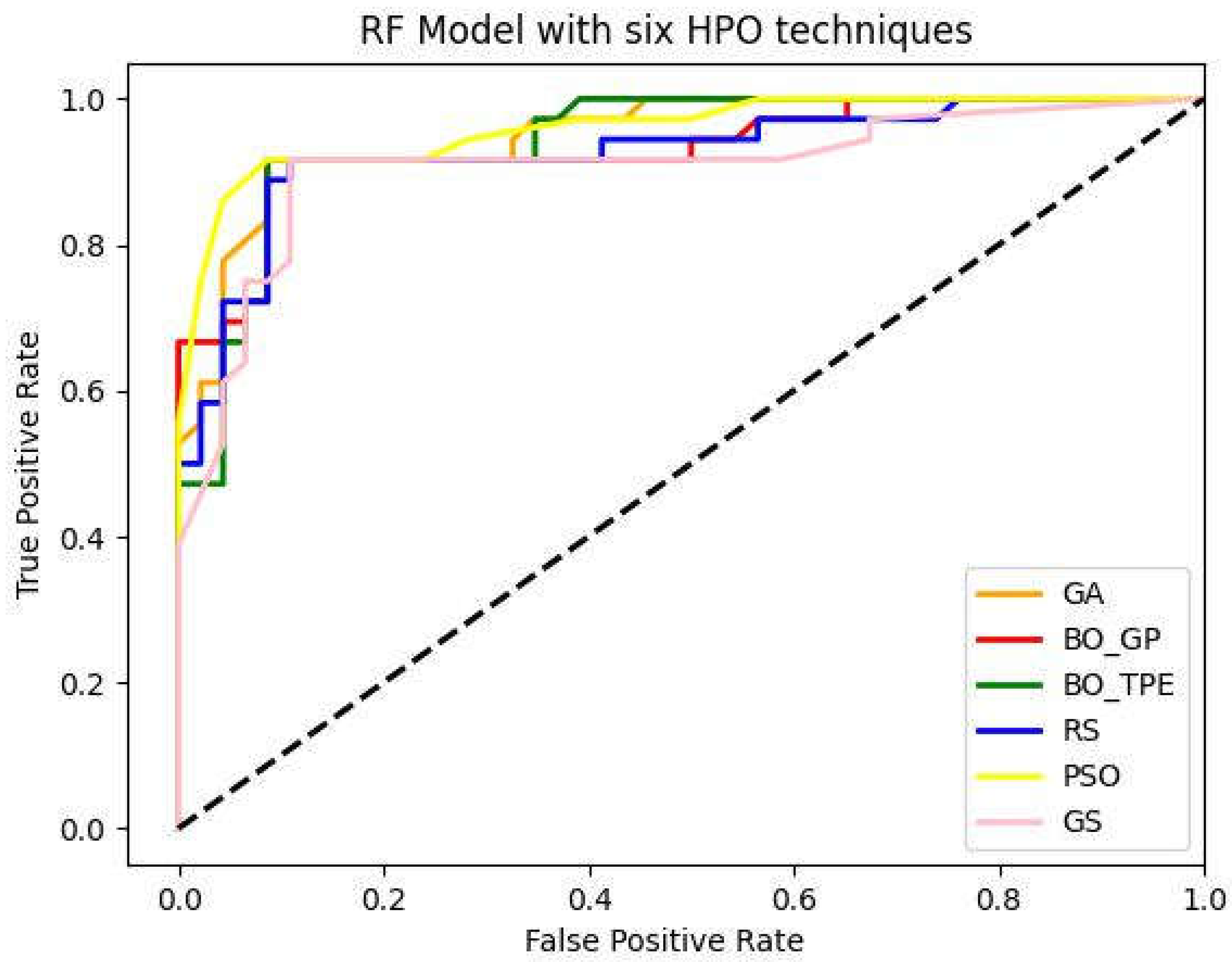
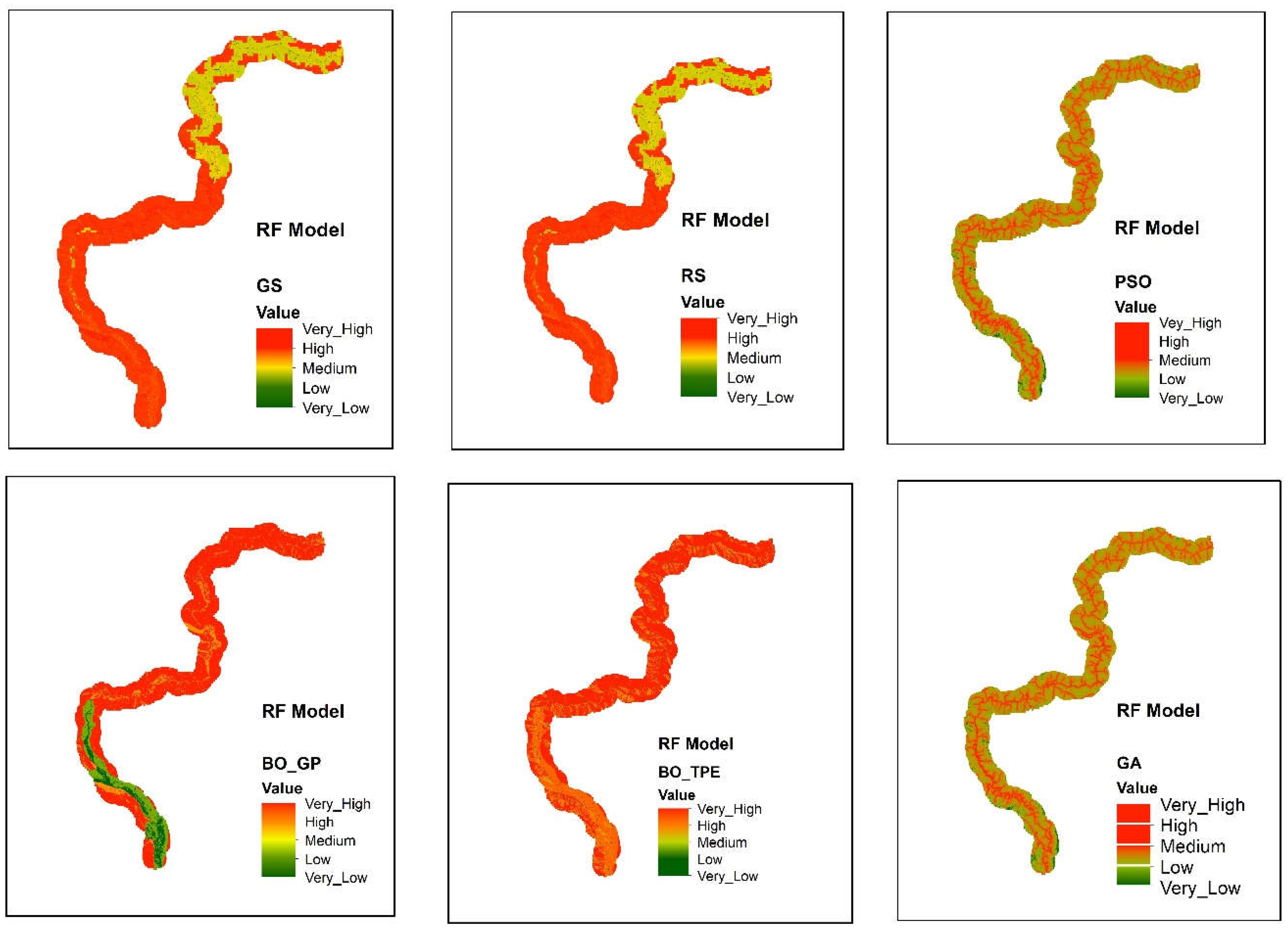
Figure 5. landslide susceptibility maps obtain from Random Forest (RF) model using six different optimization techniques GS (Grid Search), RS (Random Search), BO-GP (Bayesian optimization Gaussian process), BO-TPE (Bayesian optimization Tree-structured Parzen estimator), GA (Genetic Algorithm) and PSO (Particle Swarm Optimization).

7.1.2. KNN

Discrete hyperparameters in KNN, like the number of neighbors to take into consideration or k, are the main hyperparameters that require tuning. As explained in section (hyperparameters), Bayesian optimization is the best choice in these conditions. As expected, the Bayesian approaches performed exceptionally well. For the KNN model, BO-TPE improved accuracy from the baseline algorithms RS and GS by 1% and 11%, respectively, while BO-GP improved results from RS and GS by 2% and 12%, respectively. The metaheuristic algorithms PSO and GA both performed similarly to BO-TPE and random search (RS), respectively.

Figure 6. Receiver-operating characteristic (ROC) curve and AUC curve of K-nearest neighbors (KNN) model with GS (Grid Search), RS (Random Search), BO-GP (Bayesian optimization Gaussian process), BO-TPE (Bayesian optimization Tree-structured Parzen estimator), GA (Genetic Algorithm) and PSO (Particle Swarm Optimization) as Parameter optimization techniques.

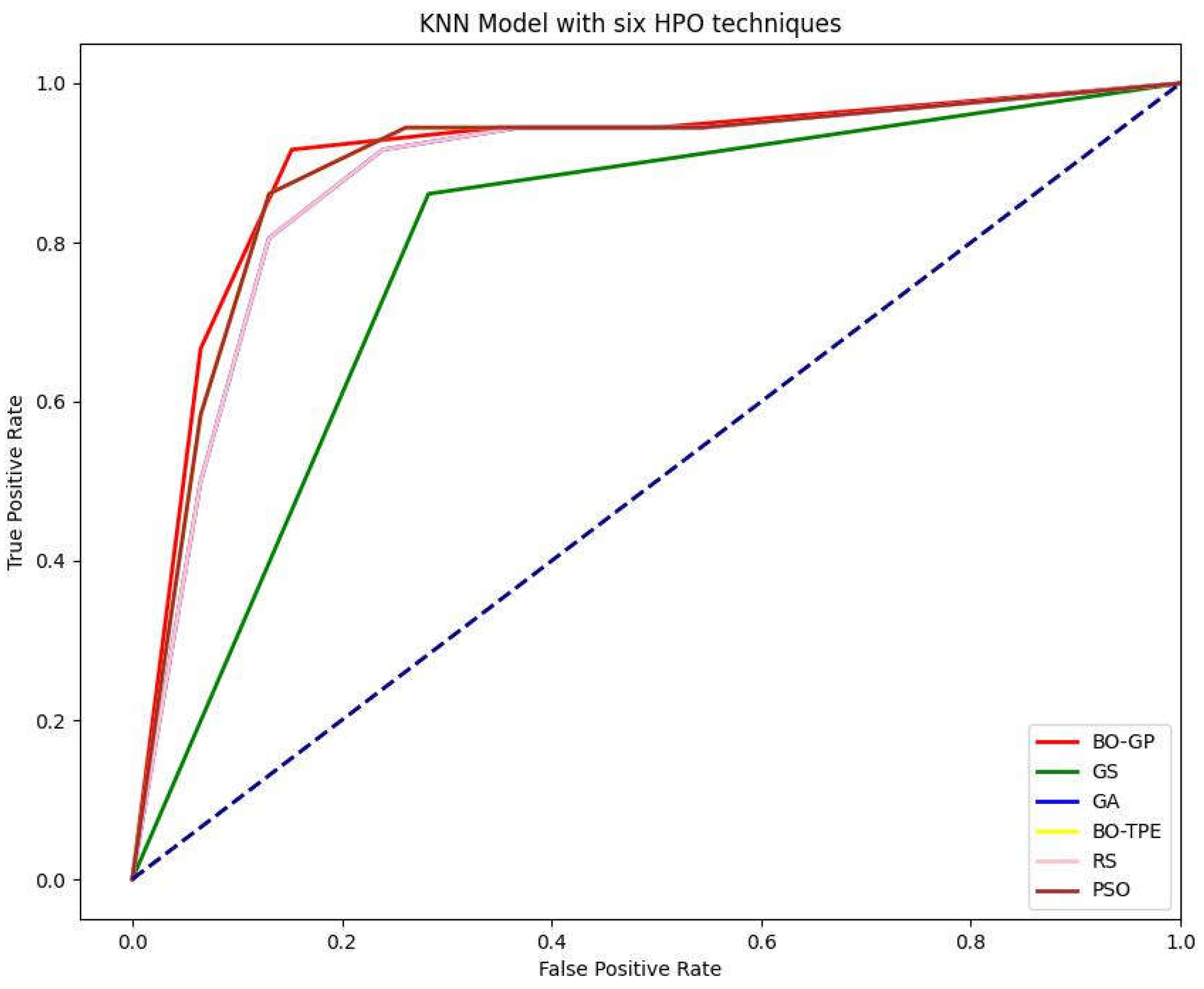
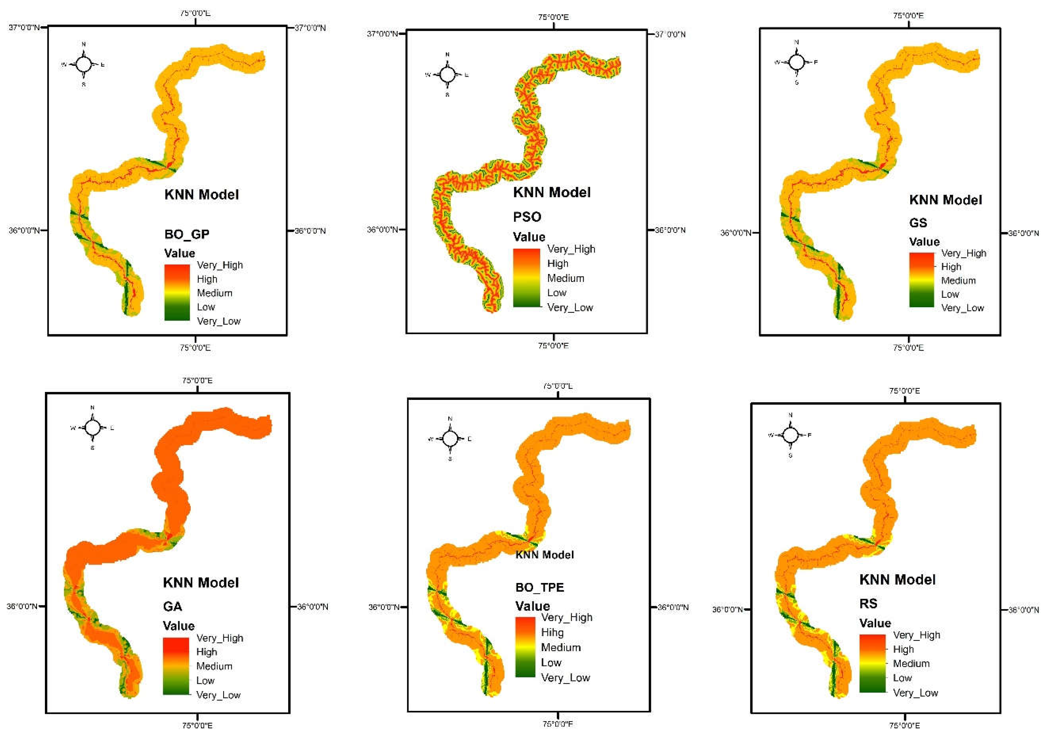
Figure 7. landslide susceptibility maps obtain from K-nearest neighbors (KNN) model using six different optimization techniques GS (Grid Search), RS (Random Search), BO-GP (Bayesian optimization Gaussian process), BO-TPE (Bayesian optimization Tree-structured Parzen estimator), GA (Genetic Algorithm) and PSO (Particle Swarm Optimization).

7.1.3. SVM

Bayesian algorithms outperformed. BO-TPE and produced 6% better outcomes than the baseline algorithms GS and RS with the SVM model. whereas BO-GP increased outcomes by 5%. PSO and GA both performed similarly, with results improving by 1% as shown in figure below.

Figure 8. Receiver-operating characteristic (ROC) curve and AUC curve of support vector machine (SVM) model with GS (Grid Search), RS (Random Search), BO-GP (Bayesian optimization Gaussian process), BO-TPE (Bayesian optimization Tree-structured Parzen estimator), GA (Genetic Algorithm) and PSO (Particle Swarm Optimization) as Parameter optimization techniques.

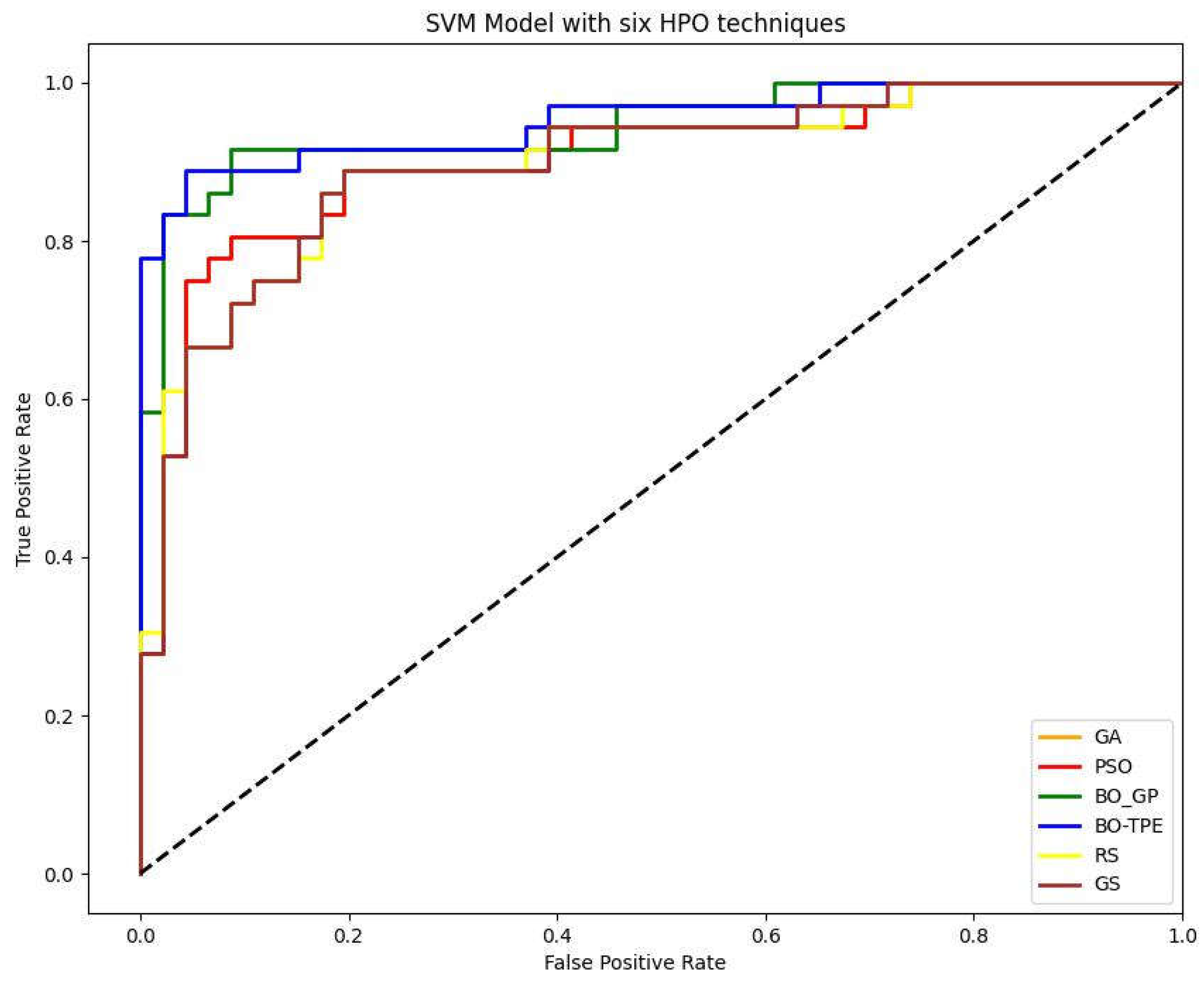
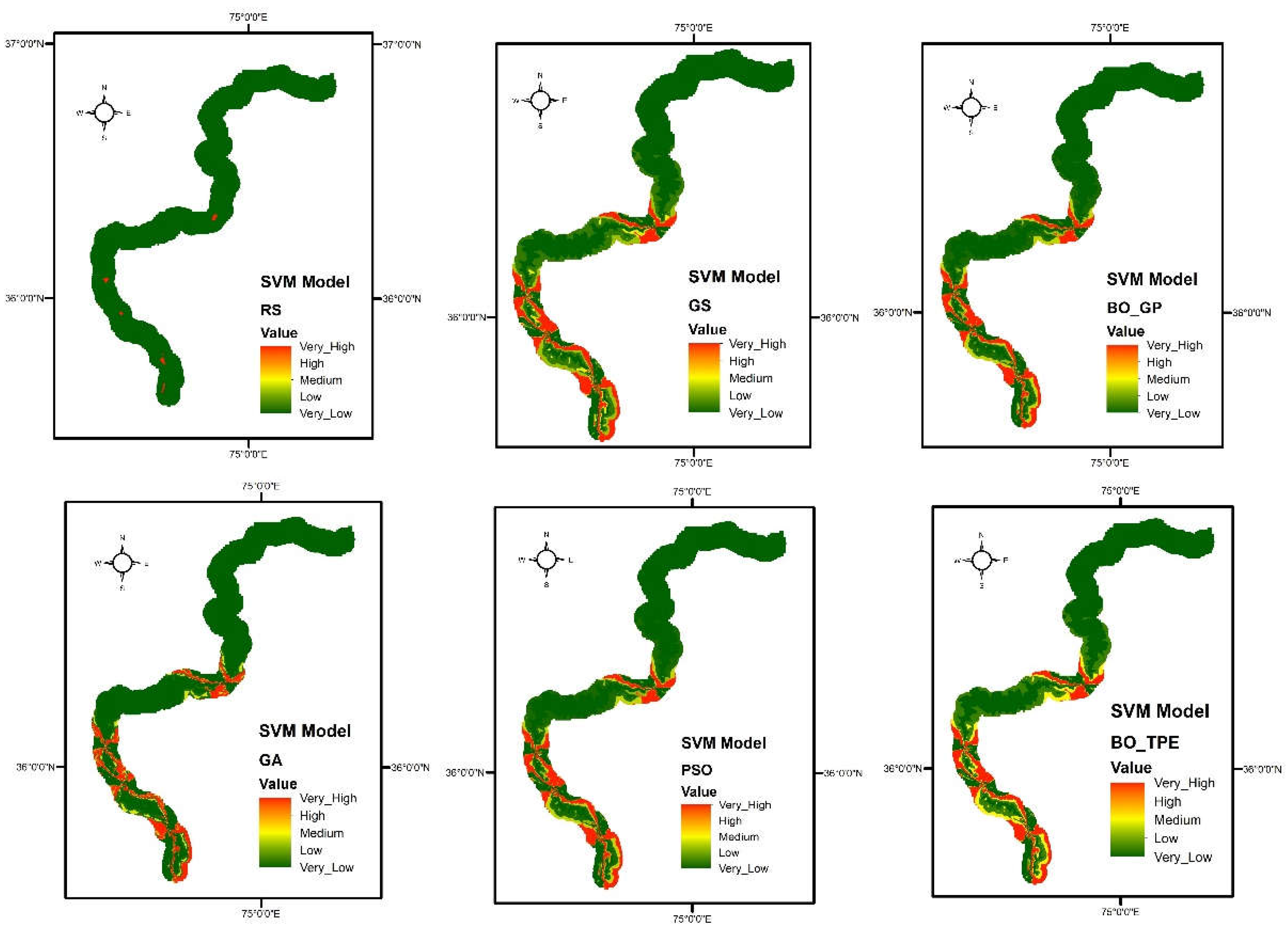
Figure 9. Landslide susceptibility maps obtain from Support Vector Machine (SVM) model using six different optimization techniques GS (Grid Search), RS (Random Search), BO-GP (Bayesian optimization Gaussian process), BO-TPE (Bayesian optimization Tree-structure Parzen estimator), GA (Genetic Algorithm) and PSO (Particle Swarm Optimization).

8. Conclusions

Machine learning is now the go-to method for solving data-related issues and is extensively employed in many applications. Their hyper-parameters must be tweaked to fit particular datasets in order to use ML models to solve practical issues. However, the size of the created data is far larger in real-life and manually adjusting hyper-parameters requires a significant investment in computer power, it is now imperative to optimize hyper-parameters through an automated method. We have thoroughly covered the most recent findings in the field of hyper-parameter optimization in this survey paper, as well as how to theoretically and practically apply them to various machine learning models. The hyper-parameter types in an ML model are the primary consideration for choosing an HPO approach when applying optimization techniques to ML models. As a result, BO models are advised for small hyper-parameter configuration spaces, while PSO is typically the ideal option for large configuration spaces. For ML data analysts, users, developers, and academics looking to apply and fine-tune ML models using appropriate HPO approaches and frameworks, we hope that our survey study will be a useful resource.

Funding

We extend our appreciation to the Researchers Supporting Project (no. RSP2023R218), King Saud University, Riyadh, Saudi Arabia.

Data Availability Statement

The data presented in the study are available on request from the first and corresponding author. The data are not publicly available due to the thesis that is being prepared from these data.

Conflicts of Interest

The authors declare no conflict of interest.

References

Polanco, C. Add a new comment. Science 2014, 346, 684–685. [Google Scholar]
Zöller, M.-A.; Huber, M.F. Benchmark and survey of automated machine learning frameworks. Journal of artificial intelligence research 2021, 70, 409–472. [Google Scholar] [CrossRef]
Elshawi, R.; Maher, M.; Sakr, S. Automated machine learning: State-of-the-art and open challenges. arXiv 2019, preprint. arXiv:1906.02287 2019. [Google Scholar]
DeCastro-García, N.; Munoz Castaneda, A.L.; Escudero Garcia, D.; Carriegos, M.V. Effect of the sampling of a dataset in the hyperparameter optimization phase over the efficiency of a machine learning algorithm. Complexity 2019, 2019. [Google Scholar] [CrossRef]
Abreu, S. Automated architecture design for deep neural networks. arXiv, 2019; preprint. arXiv:1908.10714. [Google Scholar]
Olof, S.S. A comparative study of black-box optimization algorithms for tuning of hyper-parameters in deep neural networks. 2018.
Luo, G. A review of automatic selection methods for machine learning algorithms and hyper-parameter values. Network Modeling Analysis in Health Informatics and Bioinformatics 2016, 5, 1–16. [Google Scholar] [CrossRef]
Maclaurin, D.; Duvenaud, D.; Adams, R. Gradient-based hyperparameter optimization through reversible learning. In Proceedings of the International conference on machine learning; 2015; pp. 2113–2122. [Google Scholar]
Bergstra, J.; Bardenet, R.; Bengio, Y.; Kégl, B. Algorithms for hyper-parameter optimization. Advances in neural information processing systems 2011, 24. [Google Scholar]
Bergstra, J.; Bengio, Y. Random search for hyper-parameter optimization. Journal of machine learning research 2012, 13. [Google Scholar]
Eggensperger, K.; Feurer, M.; Hutter, F.; Bergstra, J.; Snoek, J.; Hoos, H.; Leyton-Brown, K. Towards an empirical foundation for assessing bayesian optimization of hyperparameters. In Proceedings of the NIPS workshop on Bayesian Optimization in Theory and Practice; 2013. [Google Scholar]
Eggensperger, K.; Hutter, F.; Hoos, H.; Leyton-Brown, K. Efficient benchmarking of hyperparameter optimizers via surrogates. In Proceedings of the Proceedings of the AAAI Conference on Artificial Intelligence; 2015. [Google Scholar]
Li, L.; Jamieson, K.; DeSalvo, G.; Rostamizadeh, A.; Talwalkar, A. Hyperband: A novel bandit-based approach to hyperparameter optimization. The Journal of Machine Learning Research 2017, 18, 6765–6816. [Google Scholar]
Yao, Q.; Wang, M.; Chen, Y.; Dai, W.; Li, Y.-F.; Tu, W.-W.; Yang, Q.; Yu, Y. Taking human out of learning applications: A survey on automated machine learning. arXiv, 2018; preprint. arXiv:1810.13306. [Google Scholar]
Lessmann, S.; Stahlbock, R.; Crone, S.F. Optimizing hyperparameters of support vector machines by genetic algorithms. In Proceedings of the IC-AI; 2005; p. 82. [Google Scholar]
Lorenzo, P.R.; Nalepa, J.; Kawulok, M.; Ramos, L.S.; Pastor, J.R. Particle swarm optimization for hyper-parameter selection in deep neural networks. In Proceedings of the Proceedings of the genetic and evolutionary computation conference, 2017; pp. 481–488.
Ilievski, I.; Akhtar, T.; Feng, J.; Shoemaker, C. Efficient hyperparameter optimization for deep learning algorithms using deterministic rbf surrogates. In Proceedings of the Proceedings of the AAAI conference on artificial intelligence; 2017. [Google Scholar]
Claesen, M.; Simm, J.; Popovic, D.; Moreau, Y.; De Moor, B. Easy hyperparameter search using optunity. arXiv, 2014; preprint. arXiv:1412.1114. [Google Scholar]
Witt, C. Worst-case and average-case approximations by simple randomized search heuristics. In Proceedings of the STACS 2005: 22nd Annual Symposium on Theoretical Aspects of Computer Science, Stuttgart, Germany, 24–26 February 2005; Proceedings 22. pp. 44–56. [Google Scholar]
Hutter, F.; Kotthoff, L.; Vanschoren, J. Automated machine learning: methods, systems, challenges; Springer Nature: 2019.
Nguyen, V. Bayesian optimization for accelerating hyper-parameter tuning. In Proceedings of the 2019 IEEE second international conference on artificial intelligence and knowledge engineering (AIKE); 2019; pp. 302–305. [Google Scholar]
Sanders, S.; Giraud-Carrier, C. Informing the use of hyperparameter optimization through metalearning. In Proceedings of the 2017 IEEE International Conference on Data Mining (ICDM); 2017; pp. 1051–1056. [Google Scholar]
Hazan, E.; Klivans, A.; Yuan, Y. Hyperparameter optimization: A spectral approach. arXiv, 2017; preprint. arXiv:1706.00764. [Google Scholar]
Hutter, F.; Hoos, H.H.; Leyton-Brown, K. Sequential model-based optimization for general algorithm configuration. In Proceedings of the Learning and Intelligent Optimization: 5th International Conference, LION 5, Rome, Italy, 17–21 January 2011; Selected Papers 5. pp. 507–523. [Google Scholar]
Dewancker, I.; McCourt, M.; Clark, S. Bayesian optimization primer.[online] Available: https://sigopt. com/static/pdf SigOpt_Bayesian_Optimization_Primer. pdf. 2015. [Google Scholar]
Gogna, A.; Tayal, A. Metaheuristics: review and application. Journal of Experimental & Theoretical Artificial Intelligence 2013, 25, 503–526. [Google Scholar]
Itano, F.; de Sousa, M.A.d.A.; Del-Moral-Hernandez, E. Extending MLP ANN hyper-parameters Optimization by using Genetic Algorithm. In Proceedings of the 2018 International joint conference on neural networks (IJCNN); 2018; pp. 1–8. [Google Scholar]
Kazimipour, B.; Li, X.; Qin, A.K. A review of population initialization techniques for evolutionary algorithms. In Proceedings of the 2014 IEEE congress on evolutionary computation (CEC); 2014; pp. 2585–2592. [Google Scholar]
Rahnamayan, S.; Tizhoosh, H.R.; Salama, M.M. A novel population initialization method for accelerating evolutionary algorithms. Computers & Mathematics with Applications 2007, 53, 1605–1614. [Google Scholar]
Lobo, F.G.; Goldberg, D.E.; Pelikan, M. Time complexity of genetic algorithms on exponentially scaled problems. In Proceedings of the Proceedings of the 2nd annual conference on genetic and evolutionary computation, 2000; pp. 151–158.
Shi, Y.; Eberhart, R.C. Parameter selection in particle swarm optimization. In Proceedings of the Evolutionary Programming VII: 7th International Conference, EP98, San Diego, CA, USA, 25–27 March 1998; Proceedings 7. pp. 591–600. [Google Scholar]
Yan, X.-H.; He, F.-Z.; Chen, Y.-L. 基于野草扰动粒子群算法的新型软硬件划分方法. 计算机科学技术学报 2017, 32, 340–355. [Google Scholar]
Min-Yuan, C.; Kuo-Yu, H.; Merciawati, H. Multiobjective Dynamic-Guiding PSO for Optimizing Work Shift Schedules. 2018.
Wang, H.; Wu, Z.; Wang, J.; Dong, X.; Yu, S.; Chen, C. A new population initialization method based on space transformation search. In Proceedings of the 2009 Fifth International Conference on Natural Computation; 2009; pp. 332–336. [Google Scholar]
Sun, S.; Cao, Z.; Zhu, H.; Zhao, J. A survey of optimization methods from a machine learning perspective. IEEE transactions on cybernetics 2019, 50, 3668–3681. [Google Scholar] [CrossRef] [PubMed]
McCarl, B.A.; Spreen, T.H. Applied mathematical programming using algebraic systems. Cambridge, MA, 1997. [Google Scholar]
Bubeck, S. Konvex optimering: Algoritmer och komplexitet. Foundations and Trends® in Machine Learning 2015, 8, 231–357. [Google Scholar] [CrossRef]
Shahriari, B.; Bouchard-Côté, A.; Freitas, N. Unbounded Bayesian optimization via regularization. In Proceedings of the Artificial intelligence and statistics; 2016; pp. 1168–1176. [Google Scholar]
Diaz, G.I.; Fokoue-Nkoutche, A.; Nannicini, G.; Samulowitz, H. An effective algorithm for hyperparameter optimization of neural networks. IBM Journal of Research and Development 2017, 61, 9:1–9:11. [Google Scholar] [CrossRef]
Gambella, C.; Ghaddar, B.; Naoum-Sawaya, J. Optimization problems for machine learning: A survey. European Journal of Operational Research 2021, 290, 807–828. [Google Scholar] [CrossRef]
Sparks, E.R.; Talwalkar, A.; Haas, D.; Franklin, M.J.; Jordan, M.I.; Kraska, T. Automating model search for large scale machine learning. In Proceedings of the Sixth ACM Symposium on Cloud Computing, 2015; pp. 368–380.
Nocedal, J.; Wright, S.J. Numerical optimization; Springer: 1999.
Pedregosa, F.; Varoquaux, G.; Gramfort, A.; Michel, V.; Thirion, B.; Grisel, O.; Blondel, M.; Prettenhofer, P.; Weiss, R.; Dubourg, V. Scikit-learn: Machine learning in Python. the Journal of machine Learning research 2011, 12, 2825–2830. [Google Scholar]
Chen, C.; Yan, C.; Li, Y. A robust weighted least squares support vector regression based on least trimmed squares. Neurocomputing 2015, 168, 941–946. [Google Scholar] [CrossRef]
Yang, L.; Muresan, R.; Al-Dweik, A.; Hadjileontiadis, L.J. Image-based visibility estimation algorithm for intelligent transportation systems. IEEE Access 2018, 6, 76728–76740. [Google Scholar] [CrossRef]
Zhang, J.; Jin, R.; Yang, Y.; Hauptmann, A. Modified logistic regression: An approximation to SVM and its applications in large-scale text categorization. 2003.
Soliman, O.S.; Mahmoud, A.S. A classification system for remote sensing satellite images using support vector machine with non-linear kernel functions. In Proceedings of the 2012 8th International Conference on Informatics and Systems (INFOS); 2012; pp. BIO-181–BIO-187. [Google Scholar]
Safavian, S.R.; Landgrebe, D. A survey of decision tree classifier methodology. IEEE transactions on systems, man, and cybernetics 1991, 21, 660–674. [Google Scholar] [CrossRef]
Manias, D.M.; Jammal, M.; Hawilo, H.; Shami, A.; Heidari, P.; Larabi, A.; Brunner, R. Machine learning for performance-aware virtual network function placement. In Proceedings of the 2019 IEEE Global Communications Conference (GLOBECOM); 2019; pp. 1–6. [Google Scholar]
Yang, L.; Moubayed, A.; Hamieh, I.; Shami, A. Tree-based intelligent intrusion detection system in internet of vehicles. In Proceedings of the 2019 IEEE global communications conference (GLOBECOM); 2019; pp. 1–6. [Google Scholar]
Injadat, M.; Salo, F.; Nassif, A.B.; Essex, A.; Shami, A. Bayesian optimization with machine learning algorithms towards anomaly detection. In Proceedings of the 2018 IEEE global communications conference (GLOBECOM); 2018; pp. 1–6. [Google Scholar]
Arjunan, K.; Modi, C.N. An enhanced intrusion detection framework for securing network layer of cloud computing. In Proceedings of the 2017 ISEA Asia Security and Privacy (ISEASP); 2017; pp. 1–10. [Google Scholar]
Dietterich, T.G. Ensemble methods in machine learning. In Proceedings of the Multiple Classifier Systems: First International Workshop, MCS 2000 Cagliari, Italy, 21–23 June 2000, Proceedings 1, 2000; pp. 1–15.

Figure 1. Study area for our experiment.

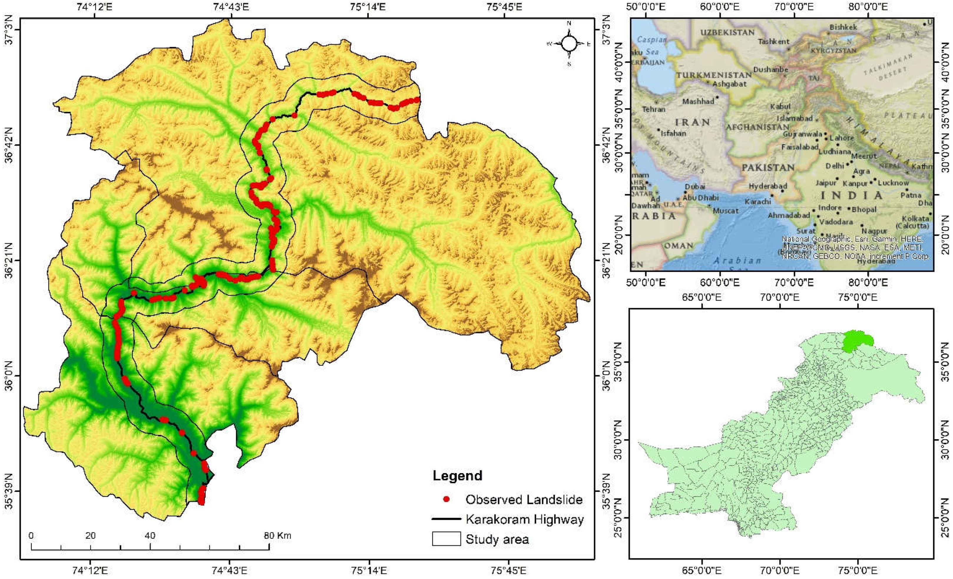
Figure 2. (a) Slope; (b) precipitation; (c) land cover; (d) aspect; (e) geology; (f) proximity to streams; (g) proximity to faults; (h) proximity to road.

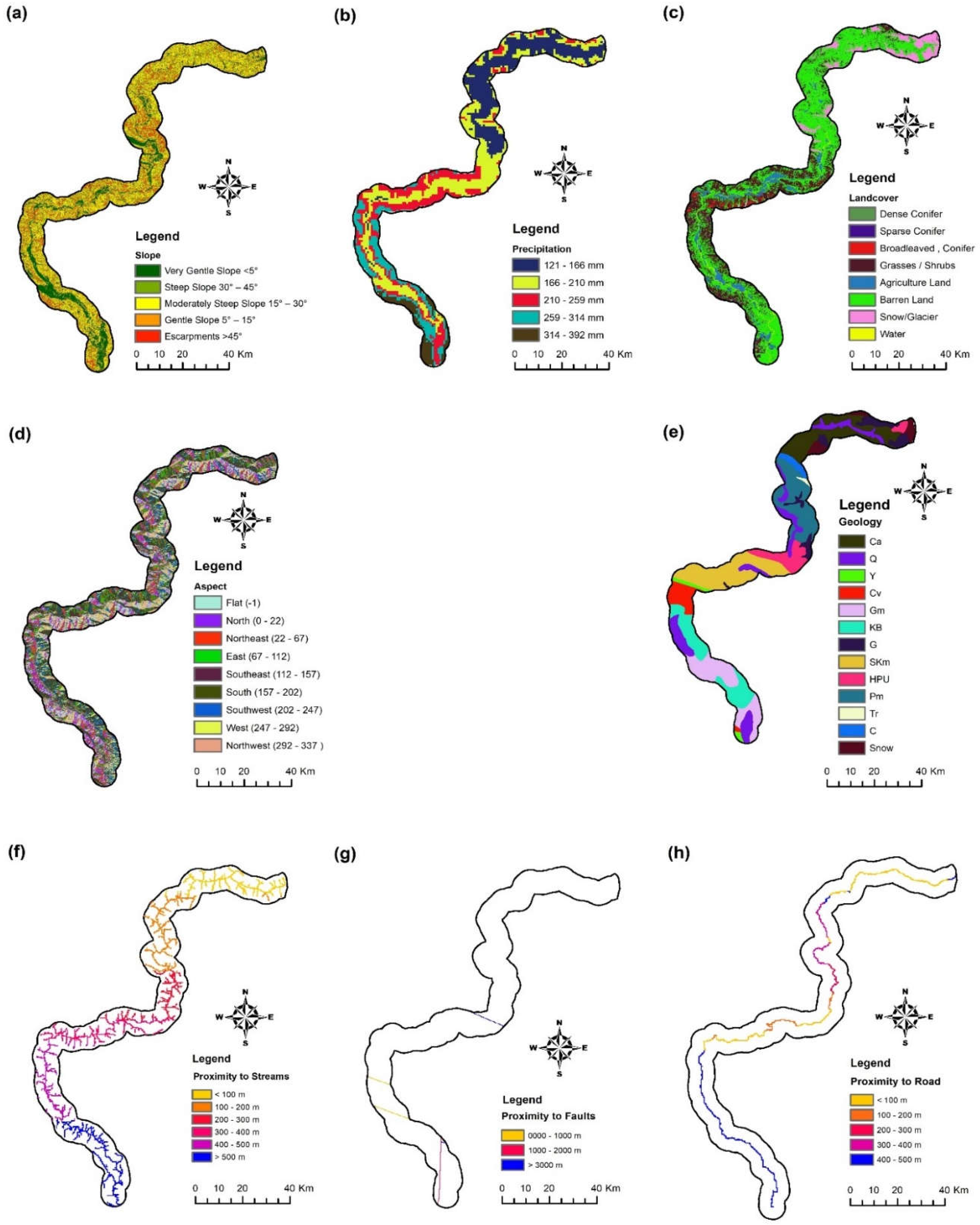
Figure 3. Methodology for hyperparameter selection for different ML algorithms for landslide susceptibility mapping.

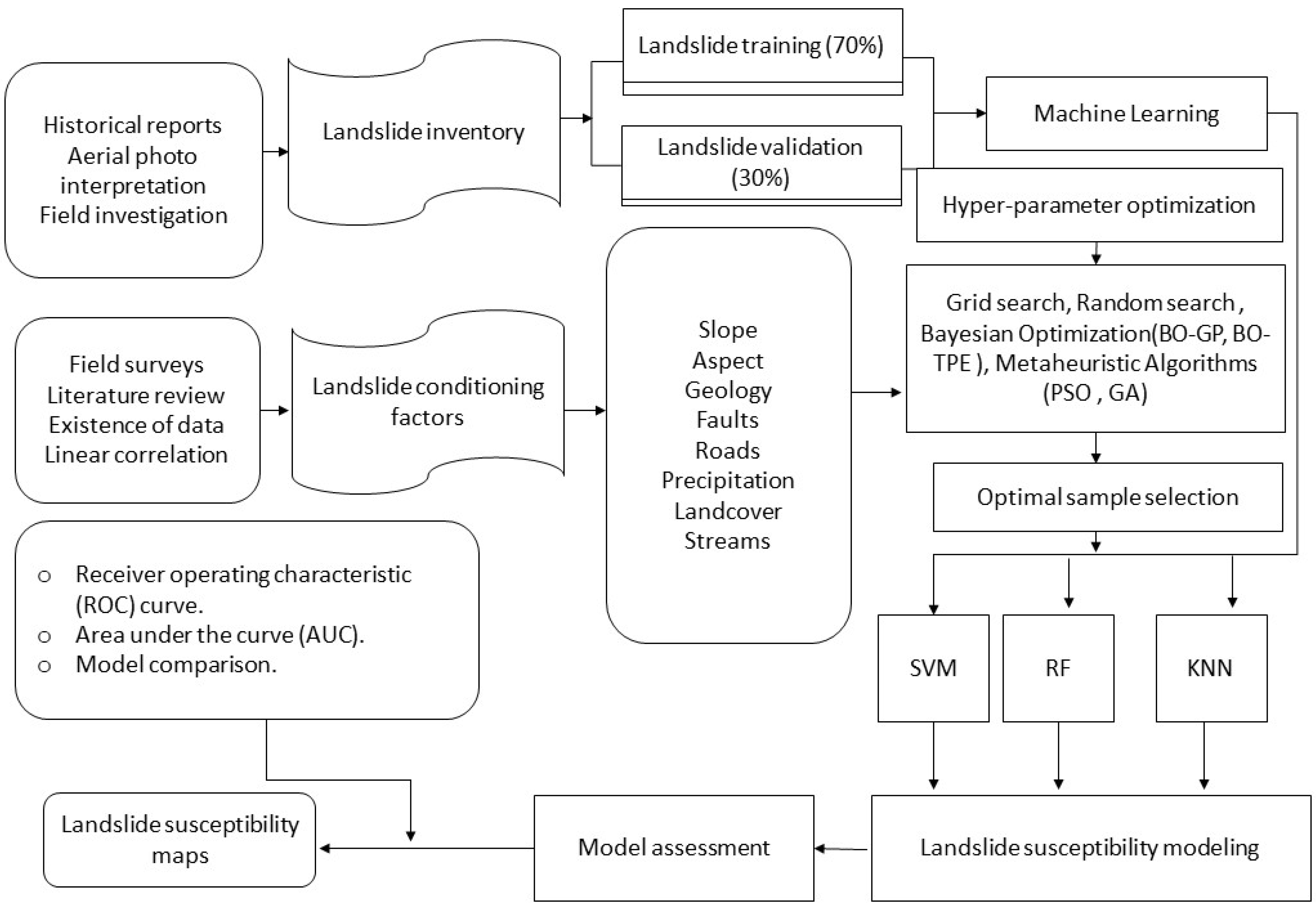
Table 1. summarized the landslide conditioning variable used in our case study.

Factors	Classes	Class Percentage %	Landslide Percentage %	Reclassification
Slope (°)	Very Gentle Slope < 5°	17.36	21.11	Geometrical interval reclassification
	Gentle Slope 5°–15°	20.87	28.37
	Moderately Steep Slope 15°–30°	26.64	37.89
	Steep Slope 30°–45°	24.40	10.90
	Escarpments > 45°	10.71	1.73
Aspect	Flat (−1)	22.86	7.04	Remained unmodified (as in source data).
	North (0–22)	21.47	7.03
	Northeast (22–67)	14.85	5.00
	East (67–112)	8.00	11.86
	Southeast (112–157)	5.22	14.3
	South (157–202)	2.84	14.40
	Southwest (202–247)	6.46	12.41
	West (247–292)	7.19	16.03
	Northwest (292–337)	11.07	11.96
Land Cover	Dense Conifer	0.38	12.73
	Sparse Conifer	0.25	12.80
	Broadleaved, Conifer	1.52	10.86
	Grasses/Shrubs	25.54	10.3
	Agriculture Land	5.78	10.40
	Soil/Rocks	56.55	14.51
	Snow/Glacier	8.89	12.03
	Water	1.06	16.96
Geology	Cretaceous sandstone	13.70	6.38
	Devonian-Carboniferous	12.34	5.80
	Chalt Group	1.43	8.43
	Hunza plutonic unit	4.74	10.74
	Paragneisses	11.38	11.34
	Yasin group	10.80	10.70
	Gilgit complex	5.80	9.58
	Trondhjemite	15.65	9.32
	Permian massive limestone	6.51	6.61
	Permanent ice	12.61	3.51
	Quaternary alluvium	0.32	8.65
	Triassic massive limestone and dolomite	1.58	7.80
	snow	3.08	2.00
Proximity to Stream (meter)	0–100 m	19.37	18.52	Geometrical interval reclassification
	100–200	10.26	21.63
	200–300	10.78	25.16
	300–400	13.95	26.12
	400–500	18.69	6.23
	>500	26.92	2.34
Proximity to Road (meter)	0–100 m	81.08	25.70
	100–200	10.34	25.19
	200–300	6.72	27.09
	300–400	1.25	12.02
	400–500	0.60	10.00
Proximity to Fault (meter)	000–1000 m	29.76	27.30
	2000–3000	36.25	37.40
	>3000	34.15	35.03

Table 2. Hyper-parameters of evaluated ML models' configuration space.

ML Model	Hyper-Parameter	Type	Search Space
RF Classifier	n_ estimators	Discrete	[10,100]
	max _depth	Discrete	[5,50]
	min _samples _split	Discrete	[2,11]
	min_ samples_ leaf	Discrete	[1,11]
	criterion	Categorical	[’gini’, ’entropy’]
	max _features	Discrete	[1,64]
SVM Classifier	C	Continuous	[0.1,50]
SVM Classifier	Kernel	Categorical	[’linear’, ’poly’, ’rbf’, ’sigmoid’]
KNN Classifier	n_ neighbors	Discrete	[1,20]

Table 3. Comparison of popular HPO algorithms (where n denotes the number of values for the hyperparameters and k the number of hyperparameters).

HPO Method	Strengths	Limitations	Time Complexity
GS	straightforward	Inefficient without categorical HPs and time-consuming.	O( $n^{k}$ )
RS	It is more effective than GS and supports parallelism.	Not taking into account prior outcomes. Ineffective when used with conditional HPs.	O(n)
BO-GP	For continuous HPs, fast convergence speed.	Poor parallelization ability; ineffective with conditional HPs	$O (n^{3})$
BO-TPE	Effective with all HP kinds. Maintain conditional dependencies.	Poor parallelization ability.	$O (n l o g n)$
GA	All HPs are effective with it, and it doesn't need excellent initialization.	Poor parallelization ability.	$O (n^{2})$
PSO	Enable parallelization; be effective with all sorts of HPs.	needs to be initialized properly.	$O (n l o g n)$

Disclaimer/Publisher’s Note: The statements, opinions and data contained in all publications are solely those of the individual author(s) and contributor(s) and not of MDPI and/or the editor(s). MDPI and/or the editor(s) disclaim responsibility for any injury to people or property resulting from any ideas, methods, instructions or products referred to in the content.

© 2023 by the authors. Licensee MDPI, Basel, Switzerland. This article is an open access article distributed under the terms and conditions of the Creative Commons Attribution (CC BY) license (https://creativecommons.org/licenses/by/4.0/).

Copyright: This open access article is published under a Creative Commons CC BY 4.0 license, which permit the free download, distribution, and reuse, provided that the author and preprint are cited in any reuse.

Submitted:

25 June 2023

Posted:

26 June 2023

You are already at the latest version

Alerts

Abstract

Keywords:

Subject: Computer Science and Mathematics - Computer Science

1. Introduction

Like numerous ML programmers devote significant time to adjusting the hyperparameters, notably for huge datasets or intricate ML algorithms having numerous hyperparameters, it decreases the degree of human labor required.
It boosts the efficacy of ML models. Numerous ML hyperparameters have diverse optimal values to attain the best results on different datasets or problems.
It boosts the replicability of the frameworks and techniques. Several ML algorithms may solely be justly assessed when the identical degree of hyper-parameter adjustment is applied; consequently, utilizing the equivalent HPO approach to several ML algorithms also assists in recognizing the ideal ML model for a specific problem.

It encompasses three well-known machine learning algorithms (SVM, RF and KNN) and their fundamental hyper-parameters.
It assesses conventional HPO methodologies, comprising their pros and cons, to facilitate their application to different ML models by selecting the fitting algorithm in pragmatic circumstances.
It investigates the impact of HPO techniques on the comprehensive precision of landslide susceptibility mapping.
It contrasts the increase in precision from the starting point and predetermined parameters to fine-tuned parameters and their impact on three renowned machine learning methods.

Study Area

Landslide Conditioning Factors

Eight different landslide conditioning factors used in our case study are presented in Figure 2 and further details of these variables are mentioned in Table 1 below.

2. Methodology

As a starting point, the landslide dataset along KKH, which is a pure classification problem, serves as the gauge dataset for the examination of the HPO method on data analysis issue.

3. Hyper-Parameters

Hyperparameter configuration characteristics can be used to categorize ML algorithms. Based on these features, suitable optimization methods can be selected to optimize the hyper-parameters.

3.1. Discrete Hyper-Parameter

3.2. Continuous Hyper-Parameter

3.3. Conditional Hyper-Parameters

3.4. Categorical Hyper-Parameters

3.5. Big Hyper-Parameter Configuration Space with Different Types of Hyper-Parameters

4. Hyper-Parameter Optimization Techniques:

4.1. Babysitting

4.2. Grid Search

GS is incapable of completely employing the fruitful zones alone. To discover the global maximum, the subsequent procedure needs to be executed manually [2]:

Commence with a wide exploration region and sizable stride length.
Utilizing prior effective hyper-parameter settings, diminish the exploration area and stride length.
Persist in repeating step 2 until the optimum outcome is achieved.

O (n^{k})

[16]. Consequently, GS can only serve as a practical HPO method when the hyper-parameter search space is limited.

4.3. Random Search

Bayesian Optimization

The following are the essential stages of Bayesian optimization (BO) [11]:

Create a surrogate probabilistic model of the target function.
Find the best hyper-parameter values on the surrogate model.
Employ these hyper-parameter values to the existing target function for evaluation.
Add the most recent observations to the surrogate model.
Repeat steps 2 through 4 until the allotted number of iterative cycles is reached.

4.4. BO-GP

μ

and a covariance

σ^{2}

[25]:

p (y| x, D) = N (y| \hat{μ}, {\hat{α}}^{2}),

(1)

BO-GP's application to a dataset of size n has a time and space complexity of

O (n^{3})

and

{O (n}^{2})

4.5. BO-TPE

l (x)

and

g (x)

, to act as generative models for entire variable range. The recorded results are divided into favorable and unfavorable outcomes based on a pre-defined percentile value

y^{*}

, and TPE is applied by utilizing simple Parzen windows [9] to model each group of results:

p (x| y, D) = \{\begin{matrix} l (x), i f y < y^{*} \\ g (x), i f y > y^{*} \end{matrix}

(2)

O (n l o g n)

[3] compared to BO-GP.

4.6. Metaheuristic Algorithms

4.7. Genetic Algorithm (GA)

The following are the primary GA procedures [26]:

Commence by randomly initializing the genes, chromosomes, and population that depict the whole exploration space, as well as the hyper-parameters and their corresponding values.
Identify the fitness function, which embodies the main objective of an ML model, and employ the findings to evaluate each member of the current generation.
Use chromosome methodologies such as crossover, mutation, and selection to generate a new generation comprising the subsequent hyper-parameter values that will be evaluated.
Continue executing steps 2 and 3 until the termination criteria are met.
Conclude the process and output the optimal hyper-parameter configuration.

O (n^{2})

time complexity [30]. GA may occasionally prove ineffective due to its slow convergence pace.

4.8. Particle Swarm Optimization (PSO)

Collection S of n particles is present in PSO as [2]:

s = (s_{1}, s_{2}, \dots \dots \dots, s_{n}),

(3)

and every particle

S_{i}

is expressed by a vector:

S_{i} = < \vec{x_{i}}, \vec{v_{i}}, \vec{p_{i}} >,

where

\vec{x_{i}}

represent the current location,

\vec{v_{i}}

represent the current speed, and

\vec{p_{i}}

is the best position of the swarm up until the current iteration.

\vec{v_{i}}

is updated rooted on its most recent global best position

\vec{p}

and its previous position

\vec{p_{i}}

\vec{v_{i}} ≔ \vec{v_{i}} + U (0, φ_{1}) (\vec{p_{i}} - \vec{x_{i}}) + U (0, φ_{2}) (\vec{p} - \vec{x_{i}}),

(4)

where the acceleration constants

φ_{1}

and

φ_{2}

are used to calculate the continuous uniform distributions

U (0, φ)

The particles then travel according to their new velocity vectors:

\vec{x_{i}} ≔ \vec{x_{i}} + \vec{v_{i}}

O (nlog n)

Hyperparameter configuration characteristics can be used to categorize ML algorithms. Based on these features, suitable optimization methods can be selected to optimize the hyper-parameters.

5. Mathematical and Hyper-Parameter Optimization

5.1. Mathematical Optimization

\min_{x \in R} f (x)

(1)

where the goal function is f(x).

\begin{matrix} \min_{x} f (x) \\ Subject to \\ g_{i} (x) \leq 0, i = 1,2, \dots \dots \dots \dots, m, \\ h_{j} (x) = 0, j = 1,2, \dots \dots \dots \dots, p, \\ x ϵ X, \end{matrix}

(2)

where X is the domain of x,

g_{i} (x) \leq 0, i = 1,2, \dots \dots \dots \dots, m,

are the inequality constraint functions, and

h_{j} (x) = 0, j = 1,2, \dots \dots \dots \dots, p,

are the equality constraint functions.

Constraints serve the purpose of limiting the feasible region, or the possible values of the optimal answer, to specific regions of the search space.

As a result, the feasible area D of x can be illustrated as follows:

D = \{x \in X| g_{i} (x) \leq 0, h_{j} (x) = 0\} .

(3)

x^{*} \in D

satisfy

f (x^{*}) \leq f (x) \forall x \in D

, whereas a local minimum is the point

x^{*} \in D

in a vicinity N satisfy

f (x^{*}) \leq f (x) \forall x \in N \cap D

[36]. As a result, the local optimum only exists in a limited range and might not be the best option for the full possible region.

f(x) is a convex function if and only if [37], for

\forall x_{1}, x_{2} \in X, \forall t \in [0,1],

f (t x_{1} + (1 - t) x_{2}) \leq f (x_{1}) + (1 - t) f (x_{2}),

(4)

\min_{x} f (x)

(5)

Subject to

x \in

5.2. Hyper-Parameter Optimization

Typically, the goal of a hyper-parameter optimization task is to get [16]:

x^{*} = a r g \min_{x \in X} f (x)

(6)

x^{*}

, is the one that results in the best value of f(x).

After choosing an ML algorithm, the primary HPO procedure involves the following steps [7]:

Choose the performance measurements and the objective function.
Identify the hyper-parameters that need tuning, list their categories, and select the optimal optimization method.
Train the ML model using the default hyper-parameter setup or common values for the baseline model.
Commence the optimization process with a broad search space, selected through manual testing and/or domain expertise, as the feasible hyperparameter domain.
If required, explore additional search spaces or narrow down the search space based on the regions where best functioning hyper-parameter values have been recently evaluated.
Finally, provide the hyper-parameter configuration that exhibits the best performance.

The majority of typical optimization approaches [40] are inappropriate for HPO However, as HPO problems differ from conventional optimization methods in the following ways [7].

6. Hyper-Parameters in Machine Learning Models

6.1. KNN

Assuming that the training set

T = \{(x_{1}, y_{1}), (x_{2}, y_{2}), \dots, (x_{n} {, y}_{n})\}

x_{i}

is the instance's feature vector and

y_{i} \in {C_{1}, C_{2}, C_{3}, \dots \dots C_{m}}

is the class of the instance,

i = (1,2, \dots . n)

, the class y of a test instance x can be represented by:

y = a r g \max_{cj} \sum_{x_{i} \in N_{k} (x)} I (y_{i} = c_{j}), i = 1,2, \dots ., n; j = 1,2 \dots ., m,

(7)

N_{k} (x)

is the field encompassing the k-nearest neighbors of x, and

I (x)

is an indicator function with I = 1 when

y_{i} = c_{j}

and I = 0 otherwise.

6.2. SVM

a r g \min_{w} \{\frac{1}{n} \sum_{i = 1}^{n} m a x {0,1 - y_{i} f (x)} + c w^{T} w\},

(8)

f (x)

used to compare two data points

x_{i}

and

x_{j}

The various kernel operations can be represented as [47]:

Linear kernel : f (x) = x_{i}^{T} x_{j};

(9)

Polynomial Kernel : f (x) = {(γ x_{i}^{T} x_{j} + γ)}^{d};

(10)

Sigmoid kernel : f (x) = (\tanh (x_{i}^{T} x_{j} + γ))

(11)

RBF kernel : f (x) = \exp (- γ {||x - x^{'}||}^{2})

(12)

γ

6.3. Random Forest (Tree Based Models)

7. Results

Performance analysis of the RF classifier using HPO methods on the landslide dataset is shown in Table 4.

Optimization Algorithm	Accuracy (%)	CT(s)
GS	0.90730	4.70
RS	0.92663	3.91
BO-GP	0.93266	16.94
BO-TPE	0.94112	1.43
GA	0.94957	4.90
PSO	0.95923	3.12

Performance analysis of the SVM classifier using HPO methods on the landslide dataset is shown in Table 5.

Optimization Algorithm	Accuracy (%)	CT(s)
BO-TPE	0.95289	0.55
BO-GP	0.94565	5.78
PSO	0.90277	0.43
GA	0.90277	1.18
RS	0.89855	0.73
GS	0.89794	1.23

Performance analysis of the KNN classifier using HPO methods on the landslide dataset is shown in Table 6.

Optimization Algorithm	Accuracy (%)	CT(s)
BO-GP	0.90247	1.21
BO-TPE	0.89462	2.23
PSO	0.89462	1.65
GA	0.88194	2.43
RS	0.88194	6.41
GS	0.78925	7.68

7.1. Landslide Susceptibility Maps

7.1.1. Random Forest

7.1.2. KNN

7.1.3. SVM

8. Conclusions

Funding

We extend our appreciation to the Researchers Supporting Project (no. RSP2023R218), King Saud University, Riyadh, Saudi Arabia.

Data Availability Statement

The data presented in the study are available on request from the first and corresponding author. The data are not publicly available due to the thesis that is being prepared from these data.

Conflicts of Interest

The authors declare no conflict of interest.

References

Polanco, C. Add a new comment. Science 2014, 346, 684–685. [Google Scholar]
Zöller, M.-A.; Huber, M.F. Benchmark and survey of automated machine learning frameworks. Journal of artificial intelligence research 2021, 70, 409–472. [Google Scholar] [CrossRef]
Elshawi, R.; Maher, M.; Sakr, S. Automated machine learning: State-of-the-art and open challenges. arXiv 2019, preprint. arXiv:1906.02287 2019. [Google Scholar]
DeCastro-García, N.; Munoz Castaneda, A.L.; Escudero Garcia, D.; Carriegos, M.V. Effect of the sampling of a dataset in the hyperparameter optimization phase over the efficiency of a machine learning algorithm. Complexity 2019, 2019. [Google Scholar] [CrossRef]
Abreu, S. Automated architecture design for deep neural networks. arXiv, 2019; preprint. arXiv:1908.10714. [Google Scholar]
Olof, S.S. A comparative study of black-box optimization algorithms for tuning of hyper-parameters in deep neural networks. 2018.
Luo, G. A review of automatic selection methods for machine learning algorithms and hyper-parameter values. Network Modeling Analysis in Health Informatics and Bioinformatics 2016, 5, 1–16. [Google Scholar] [CrossRef]
Maclaurin, D.; Duvenaud, D.; Adams, R. Gradient-based hyperparameter optimization through reversible learning. In Proceedings of the International conference on machine learning; 2015; pp. 2113–2122. [Google Scholar]
Bergstra, J.; Bardenet, R.; Bengio, Y.; Kégl, B. Algorithms for hyper-parameter optimization. Advances in neural information processing systems 2011, 24. [Google Scholar]
Bergstra, J.; Bengio, Y. Random search for hyper-parameter optimization. Journal of machine learning research 2012, 13. [Google Scholar]
Eggensperger, K.; Feurer, M.; Hutter, F.; Bergstra, J.; Snoek, J.; Hoos, H.; Leyton-Brown, K. Towards an empirical foundation for assessing bayesian optimization of hyperparameters. In Proceedings of the NIPS workshop on Bayesian Optimization in Theory and Practice; 2013. [Google Scholar]
Eggensperger, K.; Hutter, F.; Hoos, H.; Leyton-Brown, K. Efficient benchmarking of hyperparameter optimizers via surrogates. In Proceedings of the Proceedings of the AAAI Conference on Artificial Intelligence; 2015. [Google Scholar]
Li, L.; Jamieson, K.; DeSalvo, G.; Rostamizadeh, A.; Talwalkar, A. Hyperband: A novel bandit-based approach to hyperparameter optimization. The Journal of Machine Learning Research 2017, 18, 6765–6816. [Google Scholar]
Yao, Q.; Wang, M.; Chen, Y.; Dai, W.; Li, Y.-F.; Tu, W.-W.; Yang, Q.; Yu, Y. Taking human out of learning applications: A survey on automated machine learning. arXiv, 2018; preprint. arXiv:1810.13306. [Google Scholar]
Lessmann, S.; Stahlbock, R.; Crone, S.F. Optimizing hyperparameters of support vector machines by genetic algorithms. In Proceedings of the IC-AI; 2005; p. 82. [Google Scholar]
Lorenzo, P.R.; Nalepa, J.; Kawulok, M.; Ramos, L.S.; Pastor, J.R. Particle swarm optimization for hyper-parameter selection in deep neural networks. In Proceedings of the Proceedings of the genetic and evolutionary computation conference, 2017; pp. 481–488.
Ilievski, I.; Akhtar, T.; Feng, J.; Shoemaker, C. Efficient hyperparameter optimization for deep learning algorithms using deterministic rbf surrogates. In Proceedings of the Proceedings of the AAAI conference on artificial intelligence; 2017. [Google Scholar]
Claesen, M.; Simm, J.; Popovic, D.; Moreau, Y.; De Moor, B. Easy hyperparameter search using optunity. arXiv, 2014; preprint. arXiv:1412.1114. [Google Scholar]
Witt, C. Worst-case and average-case approximations by simple randomized search heuristics. In Proceedings of the STACS 2005: 22nd Annual Symposium on Theoretical Aspects of Computer Science, Stuttgart, Germany, 24–26 February 2005; Proceedings 22. pp. 44–56. [Google Scholar]
Hutter, F.; Kotthoff, L.; Vanschoren, J. Automated machine learning: methods, systems, challenges; Springer Nature: 2019.
Nguyen, V. Bayesian optimization for accelerating hyper-parameter tuning. In Proceedings of the 2019 IEEE second international conference on artificial intelligence and knowledge engineering (AIKE); 2019; pp. 302–305. [Google Scholar]
Sanders, S.; Giraud-Carrier, C. Informing the use of hyperparameter optimization through metalearning. In Proceedings of the 2017 IEEE International Conference on Data Mining (ICDM); 2017; pp. 1051–1056. [Google Scholar]
Hazan, E.; Klivans, A.; Yuan, Y. Hyperparameter optimization: A spectral approach. arXiv, 2017; preprint. arXiv:1706.00764. [Google Scholar]
Hutter, F.; Hoos, H.H.; Leyton-Brown, K. Sequential model-based optimization for general algorithm configuration. In Proceedings of the Learning and Intelligent Optimization: 5th International Conference, LION 5, Rome, Italy, 17–21 January 2011; Selected Papers 5. pp. 507–523. [Google Scholar]
Dewancker, I.; McCourt, M.; Clark, S. Bayesian optimization primer.[online] Available: https://sigopt. com/static/pdf SigOpt_Bayesian_Optimization_Primer. pdf. 2015. [Google Scholar]
Gogna, A.; Tayal, A. Metaheuristics: review and application. Journal of Experimental & Theoretical Artificial Intelligence 2013, 25, 503–526. [Google Scholar]
Itano, F.; de Sousa, M.A.d.A.; Del-Moral-Hernandez, E. Extending MLP ANN hyper-parameters Optimization by using Genetic Algorithm. In Proceedings of the 2018 International joint conference on neural networks (IJCNN); 2018; pp. 1–8. [Google Scholar]
Kazimipour, B.; Li, X.; Qin, A.K. A review of population initialization techniques for evolutionary algorithms. In Proceedings of the 2014 IEEE congress on evolutionary computation (CEC); 2014; pp. 2585–2592. [Google Scholar]
Rahnamayan, S.; Tizhoosh, H.R.; Salama, M.M. A novel population initialization method for accelerating evolutionary algorithms. Computers & Mathematics with Applications 2007, 53, 1605–1614. [Google Scholar]
Lobo, F.G.; Goldberg, D.E.; Pelikan, M. Time complexity of genetic algorithms on exponentially scaled problems. In Proceedings of the Proceedings of the 2nd annual conference on genetic and evolutionary computation, 2000; pp. 151–158.
Shi, Y.; Eberhart, R.C. Parameter selection in particle swarm optimization. In Proceedings of the Evolutionary Programming VII: 7th International Conference, EP98, San Diego, CA, USA, 25–27 March 1998; Proceedings 7. pp. 591–600. [Google Scholar]
Yan, X.-H.; He, F.-Z.; Chen, Y.-L. 基于野草扰动粒子群算法的新型软硬件划分方法. 计算机科学技术学报 2017, 32, 340–355. [Google Scholar]
Min-Yuan, C.; Kuo-Yu, H.; Merciawati, H. Multiobjective Dynamic-Guiding PSO for Optimizing Work Shift Schedules. 2018.
Wang, H.; Wu, Z.; Wang, J.; Dong, X.; Yu, S.; Chen, C. A new population initialization method based on space transformation search. In Proceedings of the 2009 Fifth International Conference on Natural Computation; 2009; pp. 332–336. [Google Scholar]
Sun, S.; Cao, Z.; Zhu, H.; Zhao, J. A survey of optimization methods from a machine learning perspective. IEEE transactions on cybernetics 2019, 50, 3668–3681. [Google Scholar] [CrossRef] [PubMed]
McCarl, B.A.; Spreen, T.H. Applied mathematical programming using algebraic systems. Cambridge, MA, 1997. [Google Scholar]
Bubeck, S. Konvex optimering: Algoritmer och komplexitet. Foundations and Trends® in Machine Learning 2015, 8, 231–357. [Google Scholar] [CrossRef]
Shahriari, B.; Bouchard-Côté, A.; Freitas, N. Unbounded Bayesian optimization via regularization. In Proceedings of the Artificial intelligence and statistics; 2016; pp. 1168–1176. [Google Scholar]
Diaz, G.I.; Fokoue-Nkoutche, A.; Nannicini, G.; Samulowitz, H. An effective algorithm for hyperparameter optimization of neural networks. IBM Journal of Research and Development 2017, 61, 9:1–9:11. [Google Scholar] [CrossRef]
Gambella, C.; Ghaddar, B.; Naoum-Sawaya, J. Optimization problems for machine learning: A survey. European Journal of Operational Research 2021, 290, 807–828. [Google Scholar] [CrossRef]
Sparks, E.R.; Talwalkar, A.; Haas, D.; Franklin, M.J.; Jordan, M.I.; Kraska, T. Automating model search for large scale machine learning. In Proceedings of the Sixth ACM Symposium on Cloud Computing, 2015; pp. 368–380.
Nocedal, J.; Wright, S.J. Numerical optimization; Springer: 1999.
Pedregosa, F.; Varoquaux, G.; Gramfort, A.; Michel, V.; Thirion, B.; Grisel, O.; Blondel, M.; Prettenhofer, P.; Weiss, R.; Dubourg, V. Scikit-learn: Machine learning in Python. the Journal of machine Learning research 2011, 12, 2825–2830. [Google Scholar]
Chen, C.; Yan, C.; Li, Y. A robust weighted least squares support vector regression based on least trimmed squares. Neurocomputing 2015, 168, 941–946. [Google Scholar] [CrossRef]
Yang, L.; Muresan, R.; Al-Dweik, A.; Hadjileontiadis, L.J. Image-based visibility estimation algorithm for intelligent transportation systems. IEEE Access 2018, 6, 76728–76740. [Google Scholar] [CrossRef]
Zhang, J.; Jin, R.; Yang, Y.; Hauptmann, A. Modified logistic regression: An approximation to SVM and its applications in large-scale text categorization. 2003.
Soliman, O.S.; Mahmoud, A.S. A classification system for remote sensing satellite images using support vector machine with non-linear kernel functions. In Proceedings of the 2012 8th International Conference on Informatics and Systems (INFOS); 2012; pp. BIO-181–BIO-187. [Google Scholar]
Safavian, S.R.; Landgrebe, D. A survey of decision tree classifier methodology. IEEE transactions on systems, man, and cybernetics 1991, 21, 660–674. [Google Scholar] [CrossRef]
Manias, D.M.; Jammal, M.; Hawilo, H.; Shami, A.; Heidari, P.; Larabi, A.; Brunner, R. Machine learning for performance-aware virtual network function placement. In Proceedings of the 2019 IEEE Global Communications Conference (GLOBECOM); 2019; pp. 1–6. [Google Scholar]
Yang, L.; Moubayed, A.; Hamieh, I.; Shami, A. Tree-based intelligent intrusion detection system in internet of vehicles. In Proceedings of the 2019 IEEE global communications conference (GLOBECOM); 2019; pp. 1–6. [Google Scholar]
Injadat, M.; Salo, F.; Nassif, A.B.; Essex, A.; Shami, A. Bayesian optimization with machine learning algorithms towards anomaly detection. In Proceedings of the 2018 IEEE global communications conference (GLOBECOM); 2018; pp. 1–6. [Google Scholar]
Arjunan, K.; Modi, C.N. An enhanced intrusion detection framework for securing network layer of cloud computing. In Proceedings of the 2017 ISEA Asia Security and Privacy (ISEASP); 2017; pp. 1–10. [Google Scholar]
Dietterich, T.G. Ensemble methods in machine learning. In Proceedings of the Multiple Classifier Systems: First International Workshop, MCS 2000 Cagliari, Italy, 21–23 June 2000, Proceedings 1, 2000; pp. 1–15.

Figure 1. Study area for our experiment.

Figure 2. (a) Slope; (b) precipitation; (c) land cover; (d) aspect; (e) geology; (f) proximity to streams; (g) proximity to faults; (h) proximity to road.

Figure 3. Methodology for hyperparameter selection for different ML algorithms for landslide susceptibility mapping.

Table 1. summarized the landslide conditioning variable used in our case study.

Factors	Classes	Class Percentage %	Landslide Percentage %	Reclassification
Slope (°)	Very Gentle Slope < 5°	17.36	21.11	Geometrical interval reclassification
	Gentle Slope 5°–15°	20.87	28.37
	Moderately Steep Slope 15°–30°	26.64	37.89
	Steep Slope 30°–45°	24.40	10.90
	Escarpments > 45°	10.71	1.73
Aspect	Flat (−1)	22.86	7.04	Remained unmodified (as in source data).
	North (0–22)	21.47	7.03
	Northeast (22–67)	14.85	5.00
	East (67–112)	8.00	11.86
	Southeast (112–157)	5.22	14.3
	South (157–202)	2.84	14.40
	Southwest (202–247)	6.46	12.41
	West (247–292)	7.19	16.03
	Northwest (292–337)	11.07	11.96
Land Cover	Dense Conifer	0.38	12.73
	Sparse Conifer	0.25	12.80
	Broadleaved, Conifer	1.52	10.86
	Grasses/Shrubs	25.54	10.3
	Agriculture Land	5.78	10.40
	Soil/Rocks	56.55	14.51
	Snow/Glacier	8.89	12.03
	Water	1.06	16.96
Geology	Cretaceous sandstone	13.70	6.38
	Devonian-Carboniferous	12.34	5.80
	Chalt Group	1.43	8.43
	Hunza plutonic unit	4.74	10.74
	Paragneisses	11.38	11.34
	Yasin group	10.80	10.70
	Gilgit complex	5.80	9.58
	Trondhjemite	15.65	9.32
	Permian massive limestone	6.51	6.61
	Permanent ice	12.61	3.51
	Quaternary alluvium	0.32	8.65
	Triassic massive limestone and dolomite	1.58	7.80
	snow	3.08	2.00
Proximity to Stream (meter)	0–100 m	19.37	18.52	Geometrical interval reclassification
	100–200	10.26	21.63
	200–300	10.78	25.16
	300–400	13.95	26.12
	400–500	18.69	6.23
	>500	26.92	2.34
Proximity to Road (meter)	0–100 m	81.08	25.70
	100–200	10.34	25.19
	200–300	6.72	27.09
	300–400	1.25	12.02
	400–500	0.60	10.00
Proximity to Fault (meter)	000–1000 m	29.76	27.30
	2000–3000	36.25	37.40
	>3000	34.15	35.03

Table 2. Hyper-parameters of evaluated ML models' configuration space.

ML Model	Hyper-Parameter	Type	Search Space
RF Classifier	n_ estimators	Discrete	[10,100]
	max _depth	Discrete	[5,50]
	min _samples _split	Discrete	[2,11]
	min_ samples_ leaf	Discrete	[1,11]
	criterion	Categorical	[’gini’, ’entropy’]
	max _features	Discrete	[1,64]
SVM Classifier	C	Continuous	[0.1,50]
SVM Classifier	Kernel	Categorical	[’linear’, ’poly’, ’rbf’, ’sigmoid’]
KNN Classifier	n_ neighbors	Discrete	[1,20]

Table 3. Comparison of popular HPO algorithms (where n denotes the number of values for the hyperparameters and k the number of hyperparameters).

HPO Method	Strengths	Limitations	Time Complexity
GS	straightforward	Inefficient without categorical HPs and time-consuming.	O( $n^{k}$ )
RS	It is more effective than GS and supports parallelism.	Not taking into account prior outcomes. Ineffective when used with conditional HPs.	O(n)
BO-GP	For continuous HPs, fast convergence speed.	Poor parallelization ability; ineffective with conditional HPs	$O (n^{3})$
BO-TPE	Effective with all HP kinds. Maintain conditional dependencies.	Poor parallelization ability.	$O (n l o g n)$
GA	All HPs are effective with it, and it doesn't need excellent initialization.	Poor parallelization ability.	$O (n^{2})$
PSO	Enable parallelization; be effective with all sorts of HPs.	needs to be initialized properly.	$O (n l o g n)$

MDPI Initiatives

Important Links

Choose an area of interest and we will send you notifications of new preprints at your preferred frequency.

Disclaimer

Hyperparameter Optimization for Landslide Susceptibility Mapping: A Comparison between Baseline, Bayesian and Metaheuristic Hyperparameter Optimization Techniques for Machine Learning Algorithms

Abstract

1. Introduction

Study Area

Landslide Conditioning Factors

2. Methodology

3. Hyper-Parameters

3.1. Discrete Hyper-Parameter

3.2. Continuous Hyper-Parameter

3.3. Conditional Hyper-Parameters

3.4. Categorical Hyper-Parameters

3.5. Big Hyper-Parameter Configuration Space with Different Types of Hyper-Parameters

4. Hyper-Parameter Optimization Techniques:

4.1. Babysitting

4.2. Grid Search

4.3. Random Search

Bayesian Optimization

4.4. BO-GP

4.5. BO-TPE

4.6. Metaheuristic Algorithms

4.7. Genetic Algorithm (GA)

4.8. Particle Swarm Optimization (PSO)

5. Mathematical and Hyper-Parameter Optimization

5.1. Mathematical Optimization

5.2. Hyper-Parameter Optimization

6. Hyper-Parameters in Machine Learning Models

6.1. KNN

6.2. SVM

6.3. Random Forest (Tree Based Models)

7. Results

7.1. Landslide Susceptibility Maps

7.1.1. Random Forest

7.1.2. KNN

7.1.3. SVM

8. Conclusions

Funding

Data Availability Statement

Conflicts of Interest

References

Abstract

1. Introduction

Study Area

Landslide Conditioning Factors

2. Methodology

3. Hyper-Parameters

3.1. Discrete Hyper-Parameter

3.2. Continuous Hyper-Parameter

3.3. Conditional Hyper-Parameters

3.4. Categorical Hyper-Parameters

3.5. Big Hyper-Parameter Configuration Space with Different Types of Hyper-Parameters

4. Hyper-Parameter Optimization Techniques:

4.1. Babysitting

4.2. Grid Search

4.3. Random Search

Bayesian Optimization

4.4. BO-GP

4.5. BO-TPE

4.6. Metaheuristic Algorithms

4.7. Genetic Algorithm (GA)

4.8. Particle Swarm Optimization (PSO)

5. Mathematical and Hyper-Parameter Optimization

5.1. Mathematical Optimization

5.2. Hyper-Parameter Optimization

6. Hyper-Parameters in Machine Learning Models

6.1. KNN

6.2. SVM

6.3. Random Forest (Tree Based Models)

7. Results

7.1. Landslide Susceptibility Maps

7.1.1. Random Forest

7.1.2. KNN

7.1.3. SVM

8. Conclusions

Funding

Data Availability Statement

Conflicts of Interest

References

MDPI Initiatives

Important Links

Subscribe