Computation of Matrix Determinants by Cross-Multiplication: A Rethinking of Dodgson’s Condensation and Reduction by Elementary Row Operations Methods

Preprint

Concept Paper

Computation of Matrix Determinants by Cross-Multiplication: A Rethinking of Dodgson’s Condensation and Reduction by Elementary Row Operations Methods

Altmetrics

Downloads

109

Views

Comments

A peer-reviewed article of this preprint also exists.

Judel Villas Protacio^*

This version is not peer-reviewed

Submitted:

25 June 2023

Posted:

27 June 2023

You are already at the latest version

Alerts

Abstract

We formulate a more straightforward, symmetry-based techniques in manually computing the determinant of any n×n matrix by revisiting Dodgson’s condensation method and strategically applying elementary row operations and the definition and properties of determinants. The result yields a more simplified mnemonical algorithm than the usual reduction by elementary row operations and co-factor expansion and with minimal terminal divisions performed compared to Dodgson’s internal divisions.

Keywords:

Subject: Computer Science and Mathematics - Mathematics

1. Introduction

The determinant is a unique number that is associated with a square matrix [1]. This determinant-square matrix one-to-one correspondence is a function

f (A) = | A |

which assigns the number |A| to a square matrix A, the value of which is determined from the entries of A. The methods of computing determinants usually presented in elementary linear algebra texts include the Leibniz’s definition, co-factor expansion, reduction by elementary row or column operations, and sometimes Dodgson’s condensation method.

Determinants by Definition

Definition 1.

The determinant of an

n \times n

matrix A denoted by

d e t [A]

or |A| is defined as

d e t (A) = Σ (\pm) {a_{1}}_{j_{1}} {a_{2}}_{j_{2}} {a_{3}}_{j_{3}} \dots {a_{n}}_{j_{n}}

(1)

where

j_{1} j_{2} j_{3} \dots j_{n}

are column numbers derived from the permutations of the set

S = {1, 2, 3, \dots, n}

The sign is taken as + for even permutation and - for odd permutation [1].

Accordingly, the determinants of simple matrices can be readily computed. The determinant of a single-entry matrix equals the entry itself,

|a_{11}| = a_{11}

. The butterfly method for

2 \times 2

matrices is so-called as the movement of computation suggests the butterfly wings, that is,

|\begin{matrix} a_{11} & a_{12} \\ a_{21} & a_{22} \end{matrix}| = a_{11} a_{22} - a_{21} a_{12}

. The Sarrus rule for

3 \times 3

matrices provides the most efficient approach in computing the determinant [2]. By Definition 1, the determinant of a

3 \times 3

is expanded as

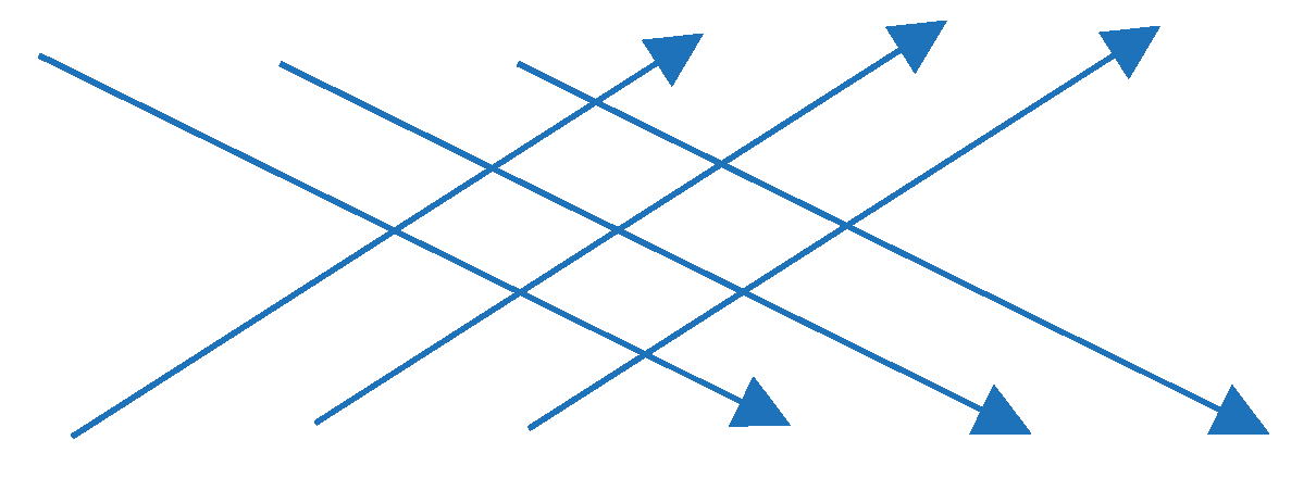
| \begin{matrix} a_{11} & a_{12} & a_{13} \\ a_{21} & a_{22} & a_{23} \\ a_{31} & a_{32} & a_{33} \end{matrix} | = a_{11} a_{22} a_{33} + a_{13} a_{21} a_{32} + a_{12} a_{23} a_{31} - a_{13} a_{22} a_{31} - a_{12} a_{21} a_{33} - a_{11} a_{23} a_{32}

(2)

By extending the first two columns of the matrix to the right, the downward arrows give the positive terms and the upward arrows give the negative terms in the expansion of the formula.

\begin{matrix} a_{11} & a_{12} & a_{13} & a_{11} & a_{12} \\ a_{21} & a_{22} & a_{23} & a_{21} & a_{22} \\ a_{31} & a_{32} & a_{33} & a_{31} & a_{32} \end{matrix}

Applying the definition in computing the determinant of

n \times n

matrix which requires

n!

terms with each containing

n

factors involving

n - 1

multiplications implies a lengthy process in manually computing the determinants as matrix size becomes larger. Several approaches were proposed to extend Sarrus rule to

4 \times 4

and

5 \times 5

matrices [2]. While these methods were shown to be efficient, the length of the process with added rules and number of factors in each term accumulate up as matrix size becomes larger.

Determinants by Cofactor Expansion

Two concepts defined below are essential in this method.

Definition 2.

The minor of an entry

a_{i j}

of an

n \times n

matrix A is the determinant of the

n - 1 \times n - 1

submatrix

M_{i j}

of A obtained by deleting the

i t h r o w a n d j t h c o l u m n

of A. The co-factor of

a_{i j}

is a real number denoted by

A_{i j}

and is defined by

A_{i j} = {(- 1)}^{i + j} \det (M_{i j})

After computing the minor and its associated co-factor, we compute the determinant by expanding about an ith row (the row containing all

a_{i j}

\det (A) = a_{i 1} A_{i 1} + a_{i 2} A_{i 2} + a_{i 3} A_{i 3} + \dots + a_{i n} A_{i n}

or jth column:

\det (A) = a_{1 j} A_{1 j} + a_{2 j} A_{2 j} + a_{3 j} A_{3 j} + \dots + a_{n j} A_{n j}

In co-factor expansion we “expand” the

n \times n

matrix about a certain row or column into

n

submatrices

M_{i j}

each with

n - 1

rows and

n - 1

columns. This means at the first expansion, we compute

n

minors and

n

co-factors. For larger matrices, we may not readily compute the minors but have to perform second expansion of each of

M_{i j}

into

n - 1

submatrices each with

n - 2

rows and

n - 2

columns; that is, the process is repeated over the resulting submatrices until smaller submatrices with readily computed determinants are obtained. The determinant of the matrix is then computed by working backward.

Determinants by Row Operations

This alternative to computing the determinants employs elementary row operations to put the matrix into upper or lower triangular form in which the resulting entries in the main diagonal lead to the calculation of the determinant. Here, we revisit the three elementary row operations and their effect on the determinant of a given matrix [1,4].

Type 1.

Multiplying a row through by a nonzero constant

Theorem 1.

B = [b_{i j}]

is the matrix that results when a single row of

A = [a_{i j}]

is multiplied by a scalar

c

, then

\det (B) = c d e t (A)

Proof:

Let

c \neq 0

be a scalar multiplier of ith row,

R_{i}

, of

A

. The definition

\det (A) = \sum (\pm) a_{1 j_{1}} a_{2 j_{2}} a_{3 j_{3}} \dots a_{n j_{n}}

denotes each entry of

R_{i}

is a factor in each term of

\sum (\pm) a_{1 j_{1}} a_{2 j_{2}} a_{3 j_{3}} \dots a_{n j_{n}}

, so that

c R_{i}

yields

\sum (\pm) c \cdot a_{1 j_{1}} a_{2 j_{2}} a_{3 j_{3}} \dots a_{n j_{n}} = c \cdot \sum (\pm) a_{1 j_{1}} a_{2 j_{2}} a_{3 j_{3}} \dots a_{n j_{n}} = c d e t (A)

Type 2.

Interchanging two rows.

Theorem 2.

B = [b_{i j}]

is the matrix that results when two rows of

A = [a_{i j}]

are interchanged, then

\det (B) = - d e t (A)

Proof:

Suppose we obtain an

n \times n

matrix

B = [b_{i j}]

by interchanging rows r and s of

A = [a_{i j}]

so that

b_{r j} = a_{s j}

and

b_{s j} = a_{r j}

. By definition,

\det (B) = \sum (\pm) b_{1 j_{1}} b_{2 j_{2}} b_{3 j_{3}} \dots b_{r j_{r}} \dots b_{s j_{s}} \dots b_{n j_{n}}

in terms of the entries of B and

\det (B) = \sum (\pm) a_{1 j_{1}} a_{2 j_{2}} a_{3 j_{3}} \dots a_{s j_{r}} \dots a_{r j_{s}} \dots a_{n j_{n}}

in terms of the entries of A. Interchanging to rows denotes a single change within the permutation and produces a change in the number of inversions as to being odd or even; hence,

\det (B) = \sum (\mp) a_{1 j_{1}} a_{2 j_{2}} a_{3 j_{3}} \dots a_{r j_{s}} \dots a_{s j_{r}} \dots a_{n j_{n}} = - \det (A)

Type 3.

Adding a constant times one row to another.

Theorem 3.

B = [b_{i j}]

is the matrix that results when a multiple of a row

R_{r}

A = [a_{i j}]

is added to another row

R_{s}

, then

\det (B) = d e t (A)

Proof.

Let

c \neq 0

be a scalar multiplier

R_{r}

so that

a_{i j} = b_{i j}

;

i \neq s

and

b_{s j} = a_{s j} + c a_{r j}

. By definition,

\begin{matrix} \det (B) & = \sum (\pm) b_{1 j_{1}} b_{2 j_{2}} b_{3 j_{3}} \dots b_{r_{j_{r}}} \dots b_{s j_{s}} \dots b_{n j_{n}} \\ = \sum (\pm) a_{1 j_{1}} a_{2 j_{2}} a_{3 j_{3}} \dots a_{r j_{r}} \dots (a_{s j_{s}} + c a_{r j_{r}}) \dots a_{n j_{n}} \end{matrix}

Expanding the summation gives

\sum (\pm) a_{1 j_{1}} a_{2 j_{2}} a_{3 j_{3}} \dots a_{r j_{r}} \dots a_{s j_{s}} \dots a_{n j_{n}} + \sum (\pm) a_{1 j_{1}} a_{2 j_{2}} a_{3 j_{3}} \dots a_{r j_{r}} \dots c a_{r j_{r}} \dots a_{n j_{n}}

Note that the first term

\sum (\pm) a_{1 j_{1}} a_{2 j_{2}} a_{3 j_{3}} \dots a_{r j_{r}} \dots a_{s j_{s}} \dots a_{n j_{n}} = d e t (A)

and

\sum (\pm) a_{1 j_{1}} a_{2 j_{2}} a_{3 j_{3}} \dots a_{r j_{r}} \dots c a_{r j_{r}} \dots a_{n j_{n}} = c \sum (\pm) a_{1 j_{1}} a_{2 j_{2}} a_{3 j_{3}} \dots a_{r j_{r}} \dots a_{r j_{r}} \dots a_{n j_{n}}

. The two equal factors denote two rows with same entries, thus

\sum (\pm) a_{1 j_{1}} a_{2 j_{2}} a_{3 j_{3}} \dots a_{r j_{r}} \dots a_{r j_{r}} \dots a_{n j_{n}} = 0

. Finally,

\det (B) = \det (A) + c (0) = d e t (A) .

By reducing a matrix into upper or lower triangular form and applying co-factor expansion, the determinant of the matrix is determined by the product of the entries in the main diagonal as stated in the following theorem.

Theorem 4.

If A =

[a_{i j}]

is upper (lower) triangular, then det(A) =

a_{11} a_{22} a_{33} \dots a_{n n}

; that is, the determinant of a triangular matrix is the product of the elements on the main diagonal.

Some methods along this approach include Chio’s condensation, triangle’s rule, Gaussian elimination procedure, LU decomposition, QR decomposition, and Cholesky decomposition (Sowabomo, 2016)

Dodgson’s Condensation Method

The English clergyman Rev. Charles Lutwidge Dodgson (1832-1898), famously known as Lewis Caroll for his literary works Alice in Wonderland and Through the Looking Glass, invented an algorithm for computing the determinant of a square matrix that is more efficient than Leibniz’s definition especially for larger matrices [4,5]. Dodgson’s method aims to ‘condense’ the determinant by producing an

(n - 1) \times (n - 1)

matrix from an

n \times n

matrix, then

(n - 2) \times (n - 2)

until a

1 \times 1

matrix is obtained. The condensation method is founded on Jacobi’s theorem [5].

Theorem 5.

Jacobi’s Theorem. Let A be an

n \times n

matrix, let

A_{i j}]

be an

m \times m

minor of

A

, where

m < n

, let

{[A'}_{i j}]

be the corresponding

m \times m

minor of

A'

, and let

[A_{i j}^{*}]

be the complementary

(n - m) \times (n - m)

minor of A. Then:

\det [{A'}_{i j}] = {\det (A)}^{m - 1} \cdot \det [A_{i j}^{*}] .

With

m = 2

, Dodgson realized that the determinant of

A

can be readily computed with

\det [A] = \frac{\det [{A'}_{i j}]}{\det [A_{i j}^{*}] .}

His algorithm consists of the following steps.

1. Check the interior of

A

for a zero entry. The interior of A is an

(n - 2) \times (n - 2)

matrix that remains when the first row, last row, first column, and last column of A are deleted. We perform elementary row operations to remove all zeros from the interior of A.

2. Compute the determinant of every four adjacent terms to form a new

(n - 1) \times (n - 1)

matrix B.

3. Repeat Step 2 to produce an

(n - 2) \times (n - 2)

matrix. We then divide each term by the corresponding entry in the interior of the original matrix A, to obtain matrix C.

4. We continue the process of condensation with the succeeding matrices a

1 \times 1

matrix obtained which gives det A.

Note that Dodgson’s method employs division of entries in succeeding matrices beginning with

(n - 2) \times (n - 2)

matrix, a step which may magnify computational error especially for matrices with non-integral entries.

Some technology-based approaches are proposed to efficiently compute the determinant. Matrices with numerically very large or small entries are scaled down to optimize computing efficiency and space; which, however may affect accuracy. Hence, some methods are proposed such as computation of determinant of square matrices without division[6]. Some matrices naturally take specialized forms which facilitate the development of formulas to compute the determinant. These include division-free algorithm to compute the determinant of quasi-tridiagonal matrices [7], development of determinant formula for special matrices involving symmetry such as block matrices [8]; break-down free algorithm for computing determinants of periodic tridiagonal matrices [9]; and block diagonalization based algorithm of block k-tridiagonal matrices [10].

The goal of this paper is to propose a more straightforward and mnemonical algorithm that can be applied to any

n \times n

numerical matrices.

2. Development of Proposed Algorithm

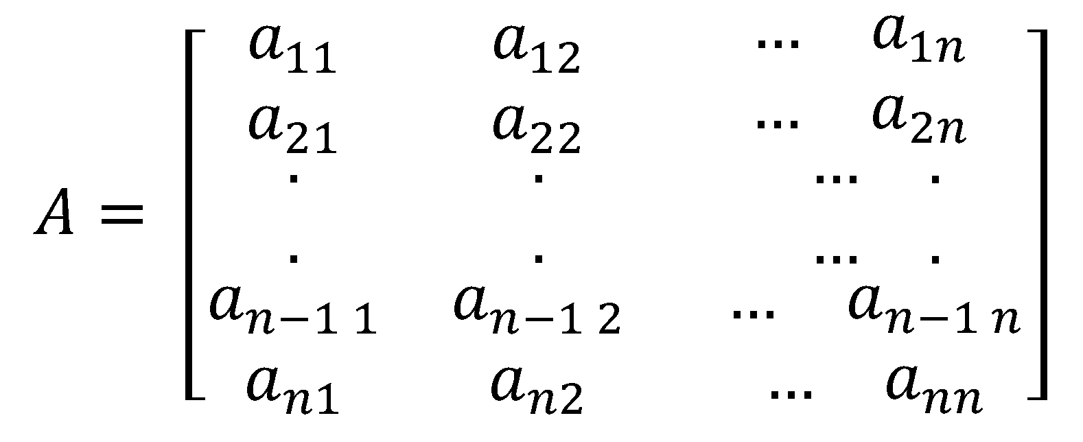
We start with an

n \times n

matrix denoted by

A_{n}

with real entries

A_{n} = [\begin{matrix} a_{11} & a_{12} & \dots & a_{1 n} \\ a_{21} & a_{22} & \dots & a_{2 n} \\ \dots \\ \dots \\ a_{n - 1 1} & a_{n - 1 2} & \dots & a_{n - 1 n} \\ a_{n 1} & a_{n 2} & \dots & a_{n n} \end{matrix}]

where the first entries are non-zero real numbers. Our goal is to produce a matrix in upper triangular form so as to readily compute the determinant by Theorem 4.

Reduction by Cross-Multiplication

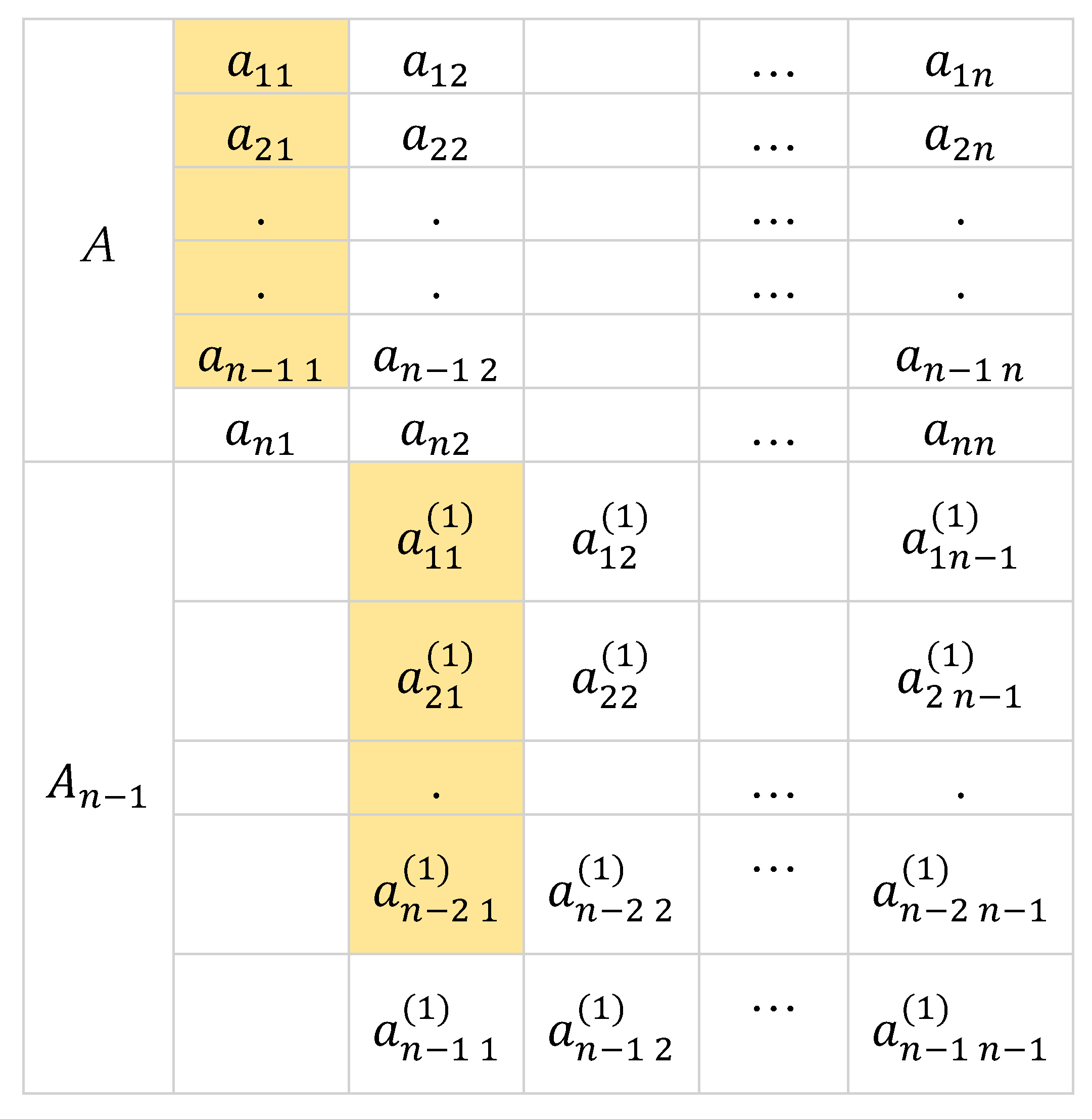
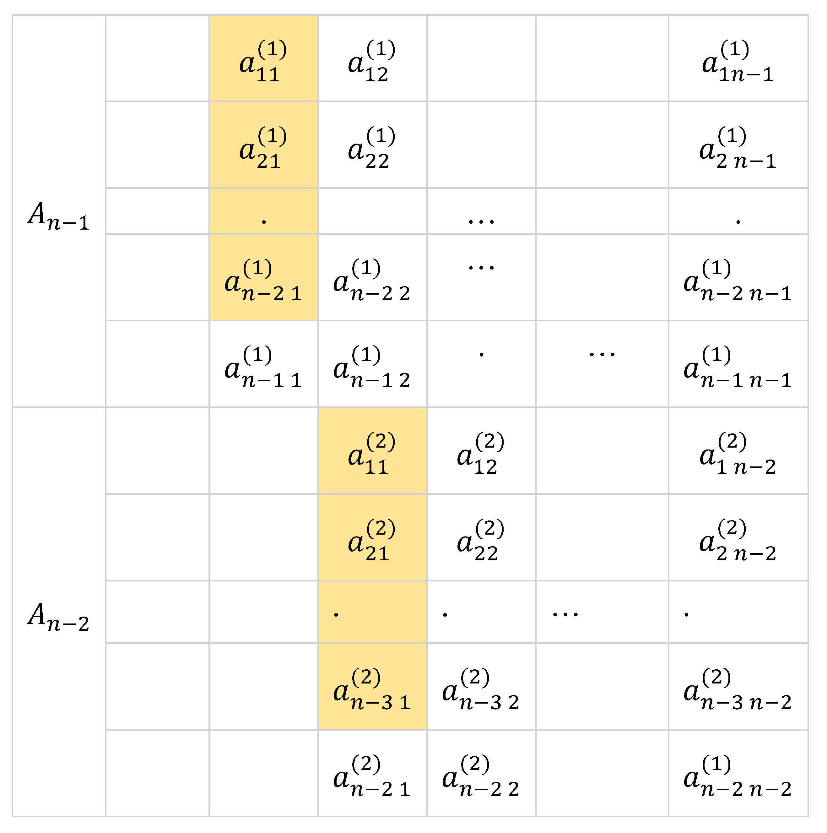
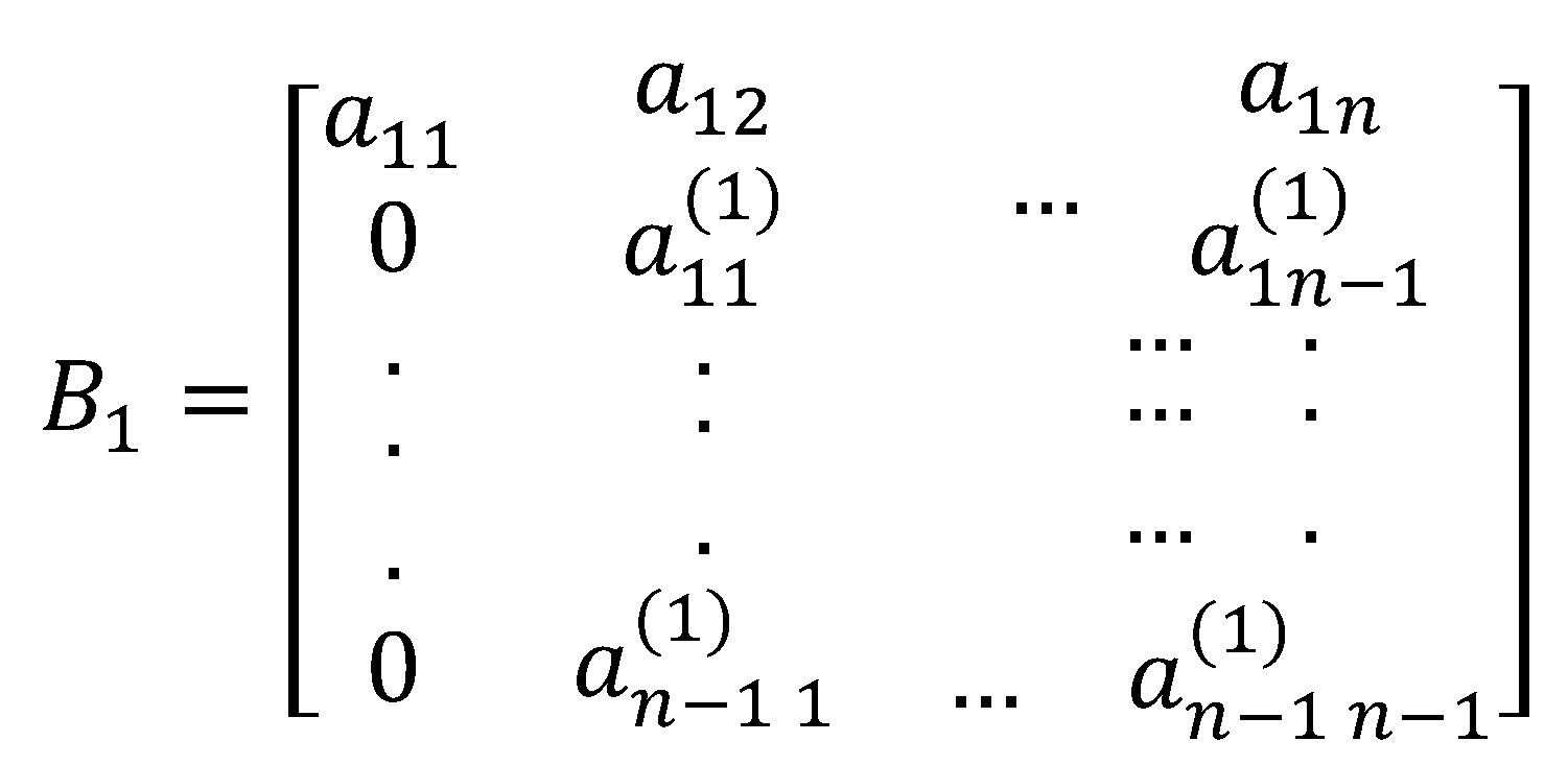
In this paper, we define reduction as the process of performing elementary row operations on a matrix to zero out entries under the first non-zero entry of the first row. A more straightforward way of zeroing out entries under

a_{11}

A

starting from the bottom row

R_{n}

is through

a_{n - 1 1} R_{n} - a_{n 1} R_{n - 1}

. By Theorem 3, the process introduces the factor

a_{n - 1 1}

into the determinant. Working our way up, we zero out the first entry of

R_{n - 1}

through

a_{n - 2 1} R_{n - 1} - a_{n - 1 1} R_{n - 2}

which then introduces the factor

a_{n - 2 1}

into the determinant. By repeating the process upward until

R_{2}

, we have introduced the following factors into the determinant of A:

a_{11}, a_{21}, \dots, a_{n - 2 1}

a_{n - 1 1} .

At this stage, we obtain a matrix

A_{n - 1}

with

n - 1

rows and

n - 1

columns by excluding the first column at the left with zero entries. We specified the entries as follows:

For the purpose of this algorithm, we do away with the usual matrix notation and we put the rows of

A_{n - 1}

under the given matrix.

The next stage is obtaining the rows for

A_{n - 2}

which is equivalent to zeroing out entries under

a_{11}^{(1)}

by following similar process done in obtaining the rows for

A_{n - 1}

. The process also introduces the following factors into the determinant:

a_{11}^{(2)}

a_{21}^{(2)}

, … ,

a_{n - 3 1}^{(2)}

a_{n - 2 1}^{(2)}

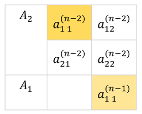
Assuming no first entries of each

A_{i}

is zero, continuing the process of reduction leads to

2 \times 2 s u b m a t r i x

A_{2}

with an introduced factor of

a_{1 1}^{(n - 2)}

and eventually

1 \times 1 s u b m a t r i x

A_{1}

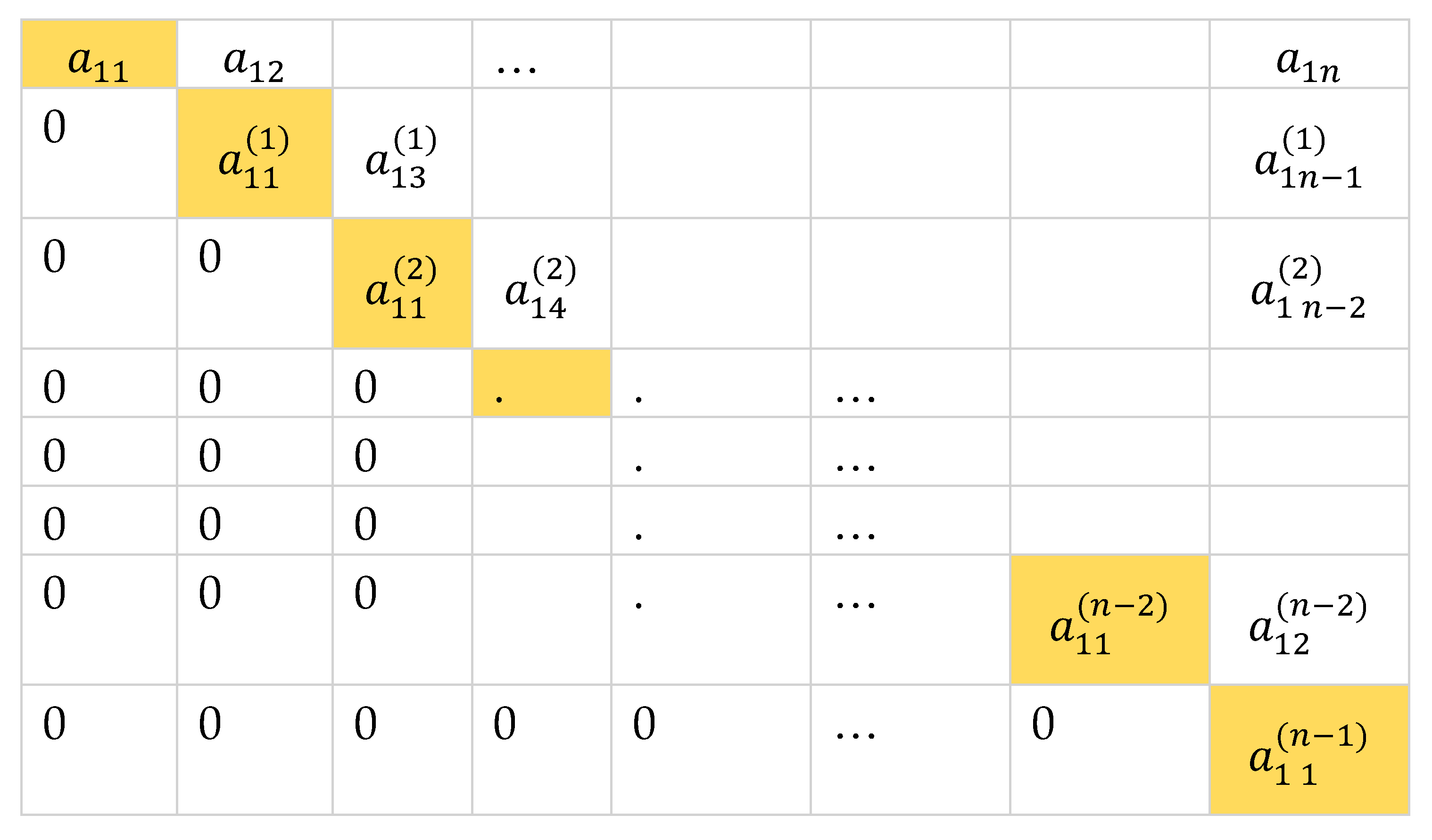
By taking the first row from each submatrix, we can reconstruct an

n \times n

matrix

B

in upper triangular form that is row equivalent to the given

n \times n

matrix

A

By Theorem 4

\det (B) = a_{11} \cdot a_{11}^{(1)} \cdot a_{11}^{(2)} \cdot \dots \cdot a_{11}^{(n - 2)} \cdot a_{11}^{(n - 1)}

Since

A

is row equivalent to

B

and these factors

a_{11} a_{21} a_{31} \dots a_{n - 11} \cdot a_{11}^{1} a_{21}^{(1)} \dots a_{n - 21}^{(1)} a_{n - 11}^{(1)} \dots a_{11}^{(n - 2)}

are introduced into the determinant of

A

in the process of forming

B

, then

from which,

Finally,

Examining the table below, the denominators are the in-between first entries in the submatrices.

Remarks.

The expression for each entry suggests a cross-multiplication pattern involving the first entries of two adjacent rows of

A

a_{i 1}

and

a_{i + 11}

, and a pair of entries in the

j t h

column,

a_{i j}

and

a_{i + 1 j}

such that a resulting entry denoted by

a_{i j - 1}^{(m)}

in the submatrix

A_{i}

is determined by

{a_{i j - 1}^{(m)} = a}_{i 1} a_{i + 1 j} - a_{i + 1 1} a_{i j}

where

(m)

is the number of reductions performed. Hence, we name this method cross-multiplication. In

A_{n - 1}

for example,

a_{11}^{(1)} = a_{11} a_{22} - a_{21} a_{12}

a_{12}^{(1)} = a_{11} a_{22} - a_{21} a_{12}

, …,

a_{1 n - 1}^{(1)} = a_{11} a_{2 n} - a_{21} a_{1 n}

, and so on until

a_{n - 1 n - 1}^{(1)} = a_{n - 1 1} a_{n n} - a_{n 1} a_{n - 1 n}

3. Cross-Multiplication and Dodgson’s Condensation Method in 3 x 3 Matrices

We now show the equivalence of Dodgson’s condensation method and cross-multiplication which as shown above is derived from elementary row operations for

3 \times 3

matrix.

Given

A = [\begin{matrix} a_{11} & a_{12} & a_{13} \\ a_{21} & a_{22} & a_{23} \\ a_{31} & a_{32} & a_{33} \end{matrix}]

where

a_{11}, a_{21}, a_{31} a n d a_{22}

are nonzero. By Dodgson’s condensation method, we take four adjacent entries at a time, compute their determinants to form a

2 \times 2

matrix.

We then compute the determinant of the resulting matrix to obtain a

1 \times 1

matrix and divide the resulting entry by the corresponding entry of the interior of

A

which is

a_{22} .

With

a_{21} a_{12} a_{32} a_{23}

cancelled, this gives

Since

a_{22}

is a common factor, then

B = a_{22} [a_{11} a_{22} a_{33} - a_{11} a_{32} a_{23} - a_{21} a_{12} a_{33} + a_{21} a_{32} a_{13} + a_{31} a_{12} a_{23} - a_{31} a_{22} a_{13}]

. By Definition 1, |A|= |

a_{11} a_{12} a_{33} - a_{11} a_{32} a_{23} - a_{21} a_{12} a_{33} + a_{21} a_{32} a_{13} + a_{31} a_{12} a_{23} - a_{31} a_{22} a_{13} |

. Thus,

|A| = \frac{| B |}{a_{22}}

By exchanging columns 1 and 2 of

A,

we have

A' = [\begin{matrix} a_{12} & a_{11} & a_{13} \\ a_{22} & a_{21} & a_{23} \\ a_{32} & a_{31} & a_{33} \end{matrix}]

and it can also be shown that

|A| = - \frac{| B' |}{a_{21}}

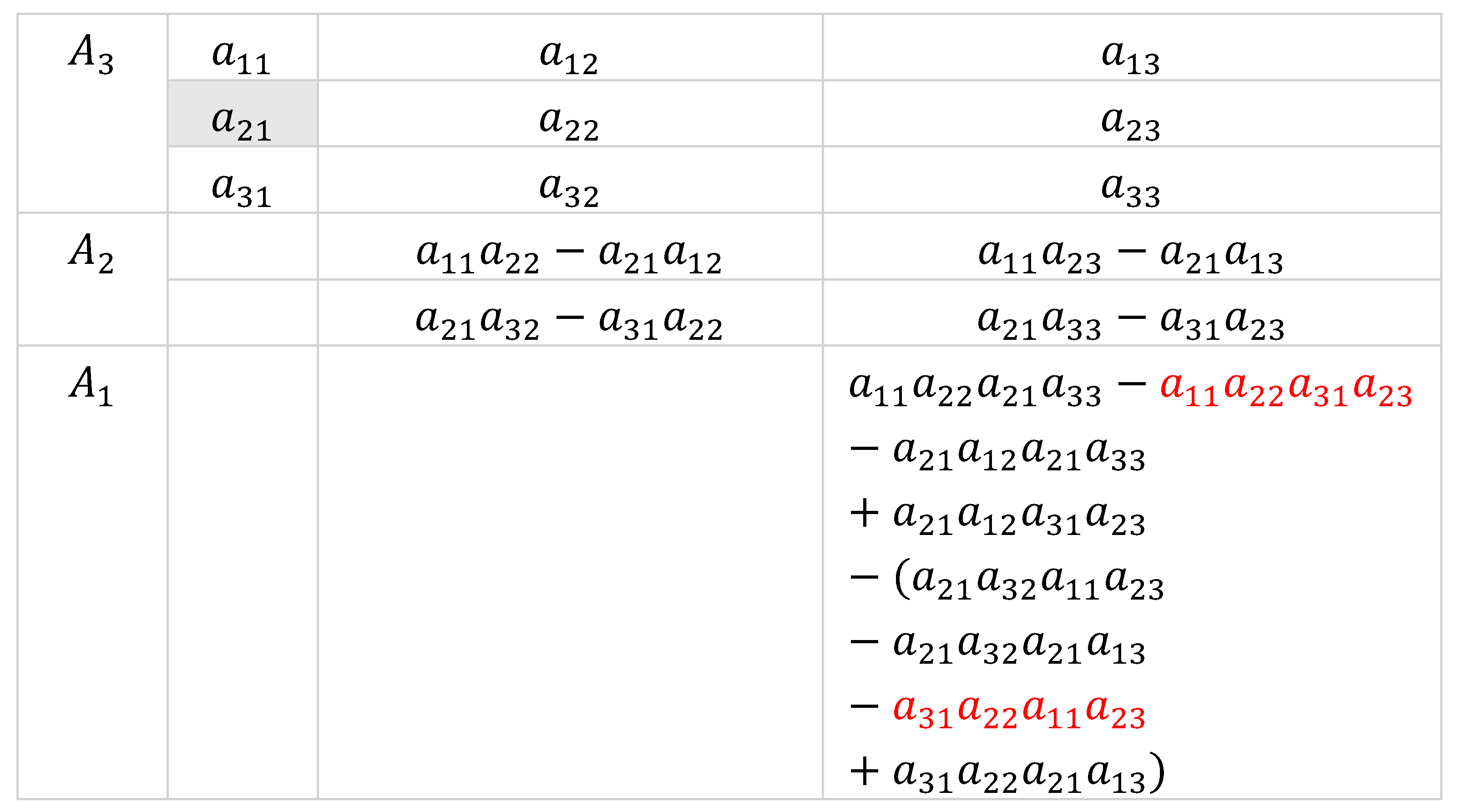
By cross-multiplication

Here,

a_{21}

is the common factor hence,

|A| = \frac{| A_{1} |}{a_{21}}

which is consistent with Equation 2.

Similar to Dodgson’s approach,

a_{i j - 1}^{(m)}

can be thought of as the determinant of

2 \times 2

matrix formed by the first entries of two adjacent rows and the pair of corresponding entries in the

j t h

column; that is,

a_{i j - 1}^{(m)} = |\begin{matrix} a_{i 1} & a_{i j} \\ a_{i + 1 1} & a_{i + 1 j} \end{matrix}|

. Here, we fix the first entries of two adjacent rows as the pivot in computing the determinants of consecutive

2 \times 2

matrices. By doing so,

a_{i + 1 1}

is the factor introduced into the original determinant, analogous to the corresponding entry of the interior matrix in the condensation method. By fixing the pivot at the first two entries, we can limit the number of divisions to be performed in preserving the determinant. With

n \geq 3 D

odgson’s method employs

n^{2} - 3 n + 1

internal divisions while cross-multiplications only employs

\frac{n^{2} - 3 n + 2}{2}

divisions at the final stage of calculations.

4. Alternate Proof of Cross-Multiplication Method

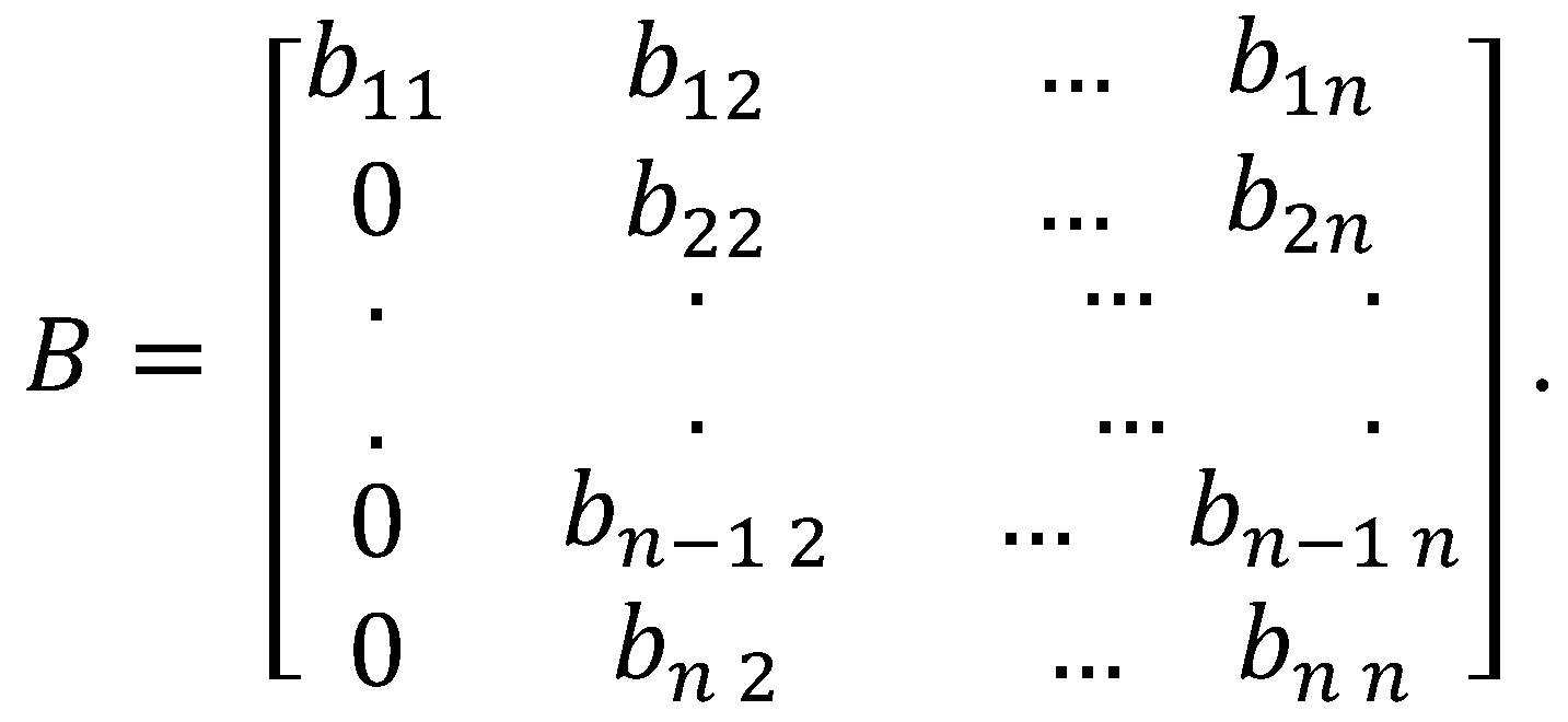
Suppose that B is an

n \times n

matrix where all entries under the first element of the first row are zeros,

By co-factor expansion

\det (B) = b_{11} {(- 1)}^{1 + 1} [\begin{matrix} b_{22} & \dots & b_{2 n} \\ . & \dots & . \\ \begin{matrix} b_{n - 1 2} \\ b_{n 2} \end{matrix} & \begin{matrix} \dots \\ \dots \end{matrix} & \begin{matrix} b_{n - 1 n} \\ b_{n n} \end{matrix} \end{matrix}]

. If

n > 4

, then to compute the determinant of the resulting

n - 1 \times n - 1

submatrix requires a full co-factor expansion or elementary row operations. In deriving the proposed method, we first transform a given matrix

A

into the form of

B

through elementary row operations then apply the definition of co-factor expansion by expanding about the first column. We then repeat the process with the succeeding submatrices until a relatively smaller matrix is obtained where we can readily compute the determinant. By introducing the cross-multiplication, we only form one

n - 1 \times n - 1

submatrix instead of

n

n - 1 \times n - 1

submatrices in co-factor expansion.

Let

A

be an

n \times n

matrix with real entries where

a_{11}, a_{21}, a_{n - 11}, a_{n 1} \neq 0 .

We zero out entries under

a_{11}

through the process illustrated in this paper: With two successive rows

R_{i}

and

R_{i + 1}

with first entries

a_{i 1}

and

a_{i + 11}

, respectively, and by

a_{i 1} R_{i + 1} - a_{i + 1 1} R_{i}

, a matrix

B_{1}

is produced.

In the process, the factors

a_{11}, a_{21}, a_{31}, \dots, a_{n - 1 1}

are introduced into

\det [A] .

Thus by Theorem 1,

By cofactor expansion,

where

A_{n - 1} = [\begin{matrix} a_{11}^{(1)} & \dots & a_{1 n - 1}^{(1)} \\ \dots & \dots & \dots \\ a_{n - 11}^{(1)} & \dots & a_{n - 1 n - 1}^{(1)} \end{matrix}]

We repeat the process of reduction on

A_{n - 1}

to form the matrix

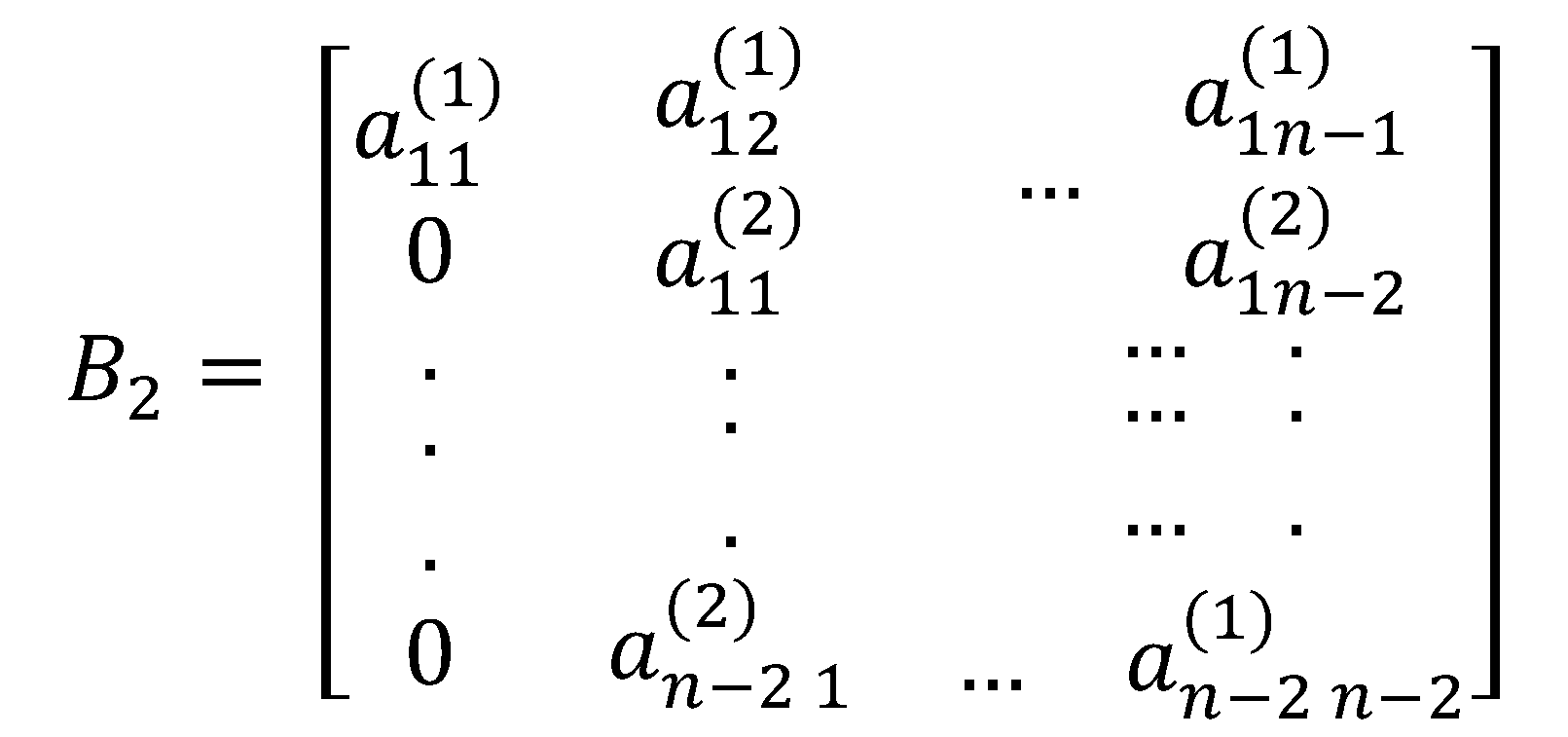
and which

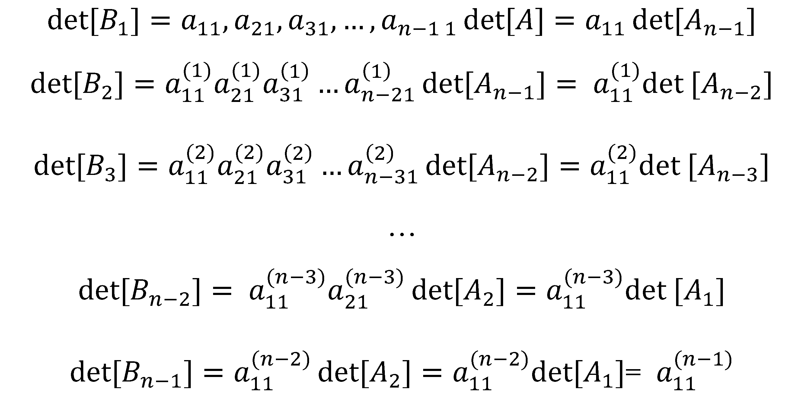
Continuing the reduction on subsequent submatrices we summarize the following results

Working backwards leads to

Hence,

5. Some Special Cases

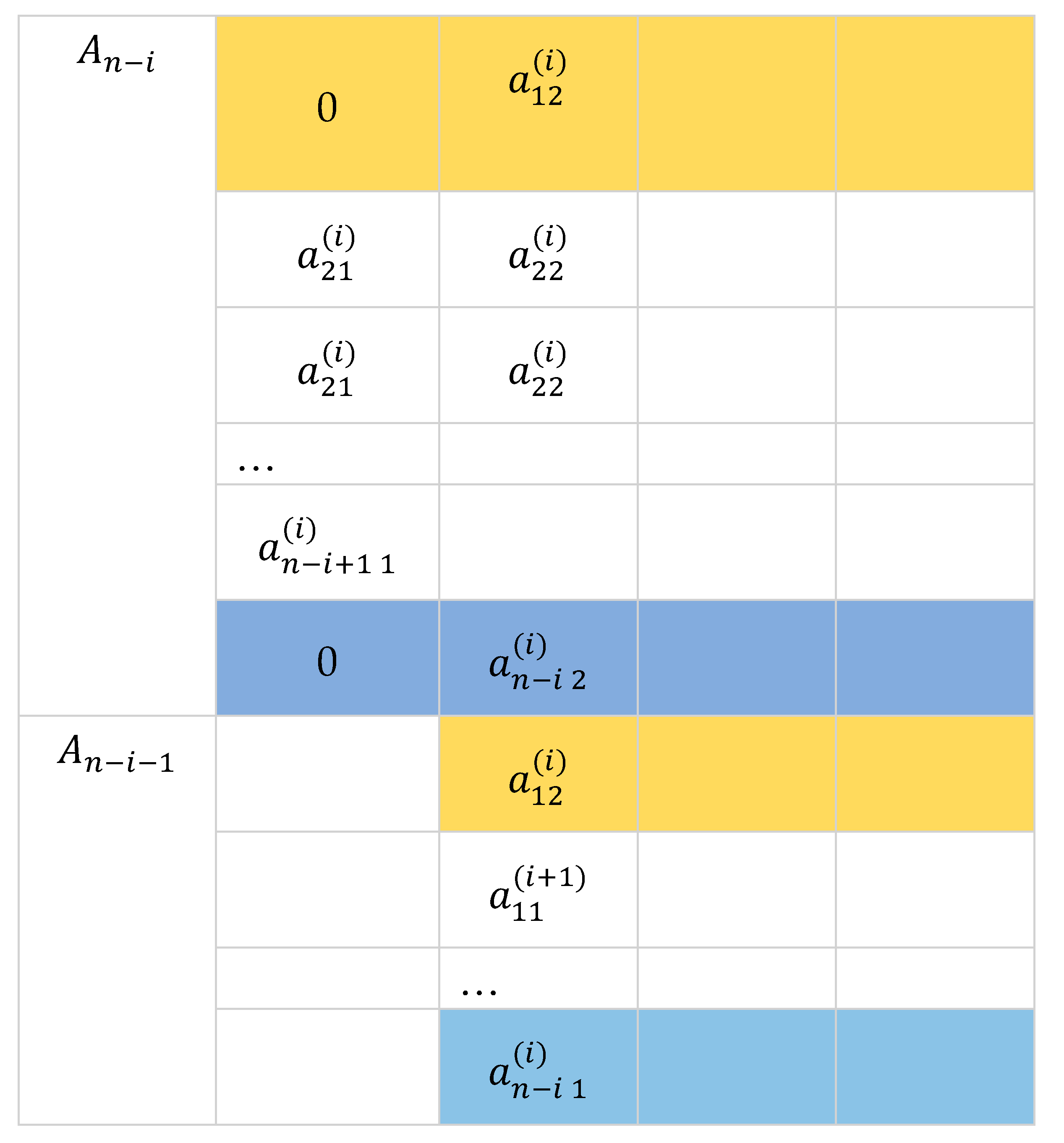
The equation in computing the determinant with the developed method holds if none of the first entries in any row is zero. Here we consider cases where there are zero first entries in any of the submatrices

A_{n - i}

Zero First Entries of First or Last Row of $A_{n - i}$ ; $n - i > 1$

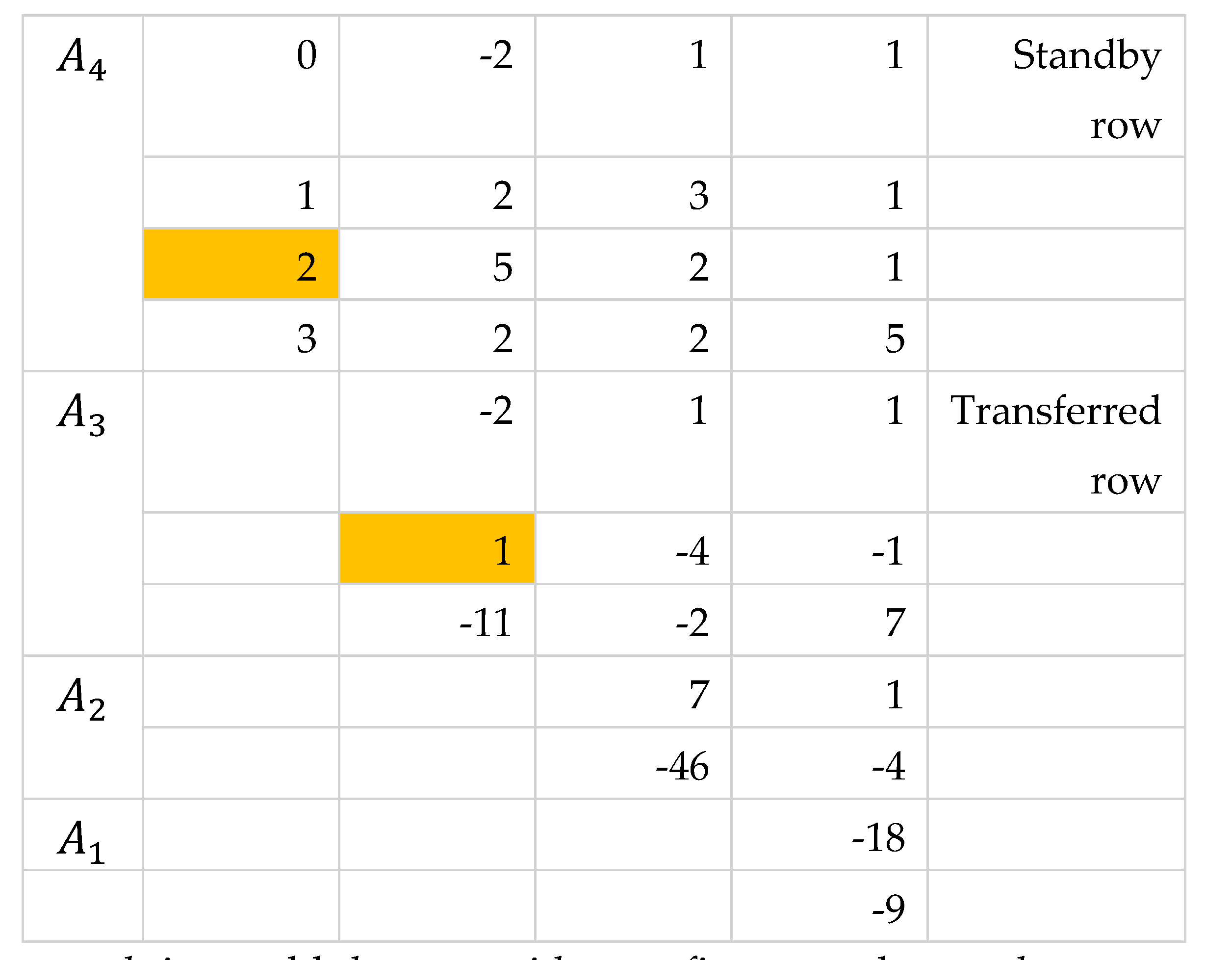
If the first entry of either first or last row of

A_{n - i}

except the last submatrix

A_{1}

is zero, then Equation 2 still holds. These rows with zero first entries are considered standby rows and do not participate in row reduction. They are then transferred to the next submatrix retaining their placement as first or last row.

By Theorem 3, we can also add any row with nonzero first entry to a row with zero first entry and go on with the usual process of reduction.

Some In-Between First Entries are Zeros

The general approach is to apply Theorem 3 by adding any row with nonzero first entry to a row with zero first entry. We can also apply Theorem 2 to lessen the number of operations especially when there are more rows with zero first entries than rows with nonzero first entries. If an

m

th row of

A_{n - i}

has

a_{m 1}^{(i)} = 0

, then the reduction

a_{m 1}^{(i)} R_{m + 1} - a_{m + 1 1}^{(i)} R_{m}

is not possible since this will introduce a zero factor in the divisor of Equation 2. We reduce the entire submatrix by first moving the rows with zero first entries to the bottom part then perform reduction to rows with nonzero first entries. The rows with zero first entries are treated as “standby rows” and are then moved to the next submatrix in the same placement. Since

\det (A_{n - i}) = a_{11}^{(k)} d e t (A_{n - i - 1})

, by Theorem 2, interchanging

R_{m}

and the last row will lead to

\det (A_{n - i}) = {- a}_{11}^{(k)} d e t (A_{n - i - 1})

. We introduce the factor

{(- 1)}^{k}

to Equation 2 where

k

indicates the number of row exchanges performed.

Only One Row Has Non-zero First Entry

If only one row of

A_{n - i}

has non-zero first entry, we place this row as

R_{1}

with first entry

a_{11}^{(n - i)}

. No reduction is performed since the

A_{n - i}

already takes the reduced form. By Theorem 4,

a_{11}^{(n - i)}

is a diagonal entry thus this leads to the modified formula:

All Rows Have Zero First Entries

If all rows of

A_{n - i}

have zero first entries, then no reduction is performed and since

a_{11}^{(n - i)} = 0,

then by Equation 2,

\det (A) = 0 .

6. Conclusions

The cross-multiplication method of computing the determinants is a mnemonical use of elementary row operations in reducing a matrix to lower triangular form by using the first entries of adjacent rows as scalar multipliers. Doing so retains the butterfly movement in computing the determinant of

2 \times 2

matrix as each entry is easily computed through

{a_{i j - 1}^{(m)} = a}_{i 1} a_{i + 1 j} - a_{i + 1 1} a_{i j}

a_{i j - 1}^{(m)} = |\begin{matrix} a_{i 1} & a_{i j} \\ a_{i + 1 1} & a_{i + 1 j} \end{matrix}|

such that

a_{i 1}

and

a_{i + 1 1}

are the pivot entries. The algorithm proceeds by computing each entry to produce a submatrix that is one row and one column less than the preceding submatrix until a

1 \times 1

matrix, [

a_{11}^{(n - 1)}],

is obtained. The determinant is then computed as to the following cases.

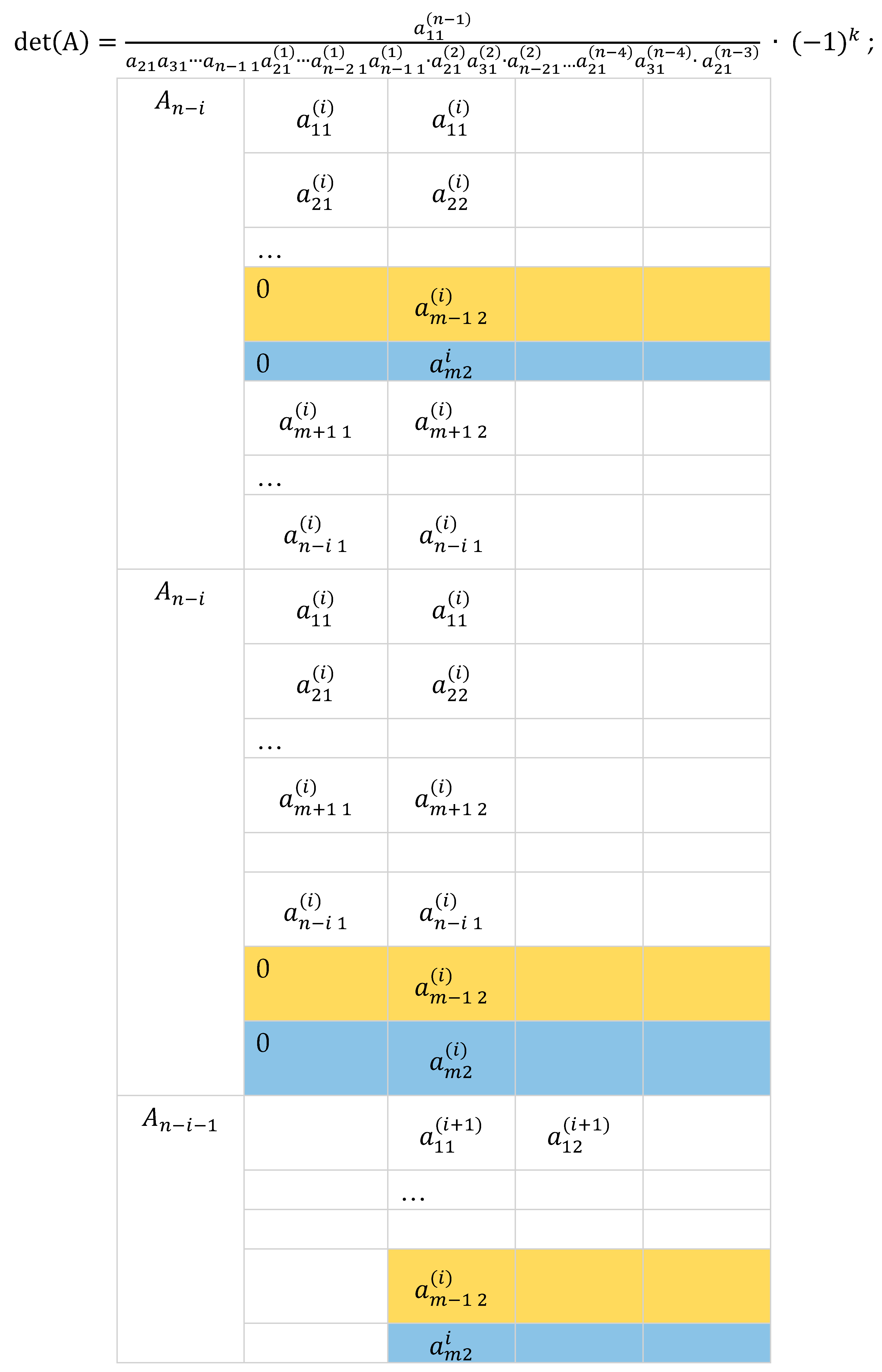
1. When all first entries in the rows of submatrices are nonzero, the determinant is solved by

\det (A) = \frac{a_{11}^{(n - i)}}{a_{21} a_{31} \dots a_{n - 11} a_{21}^{(1)} \dots a_{n - 21}^{(1)} a_{n - 11}^{(1)} \cdot a_{21}^{(2)} a_{31}^{(2)} \cdot a_{n - 21}^{(2)} \dots a_{21}^{(n - 4)} a_{31}^{(n - 4)} \dots a_{21}^{(n - 3)}}

where the factors in the denominator are the nonzero in-between first entries of submatrices, representing the factors introduced into the original determinant in the reduction process.

2. When some first entries in the rows are zero, the rows are transferred to the bottom of the submatrix and then transferred to the next submatrix. The determinant is solved by

\det (A) = \frac{a_{11}^{(n - i)}}{product of nonzero in - between first entries} \cdot {(- 1)}^{k}

where

k

is the number of row exchanges.

3. When rows with zero first entries are added by rows with nonzero first entries, the formula in (1) holds.

4. When each of the submatrices

A_{n - i}, A_{n - j}, A_{n - k}, \dots

has exactly one row with nonzero first entry, we set these rows as first rows where necessary and compute the determinant by

\det (A) = \frac{a_{11}^{(n - i)} \cdot a_{11}^{(n - j)} \cdot a_{11}^{(n - k)} \cdot \dots \cdot a_{11}^{(n - 1)}}{product of nonzero in - between first entries} \cdot {(- 1)}^{k}

where

k

is the number of row exchanges.

4. When all rows of a submatrix

A_{n - i}

have zero first entries, then

\det [A] = 0 .

For

n = 3

, cross-multiplication and Dodgson’s condensation method are shown to be equivalent. Unlike the condensation method which employs

n^{2} - 3 n + 1

internal divisions, the proposed method employs much fewer,

\frac{n^{2} - 3 n + 2}{2}

, terminal divisions thus minimizing the propagation of computational errors. Both methods require row adjustments whenever there are zero pivot entries.

Compared to co-factor expansion which generates

n

number of

(n - 1) \times (n - 1)

submatrices, then

n (n - 1)

number of

(n - 2) \times (n - 2)

submatrices, and so on, the cross-multiplication method generates only one of each of

(n - 1) \times (n - 1), (n - 2) \times (n - 2)

, …

(2 \times 2), a n d (1 \times 1)

submatrices.

The simplicity and efficiency of the proposed methods lies in the consistency and symmetry of of its iterative process. No procedural adjustments are introduced as the matrix size increases compared to other methods such as extension of Sarrus rule to matrices with

n \geq 4 .

Acknowledgments

The author acknowledges the invaluable service of peer reviewers of this paper.

Conflicts of Interest

The author declares no conflict of interest.

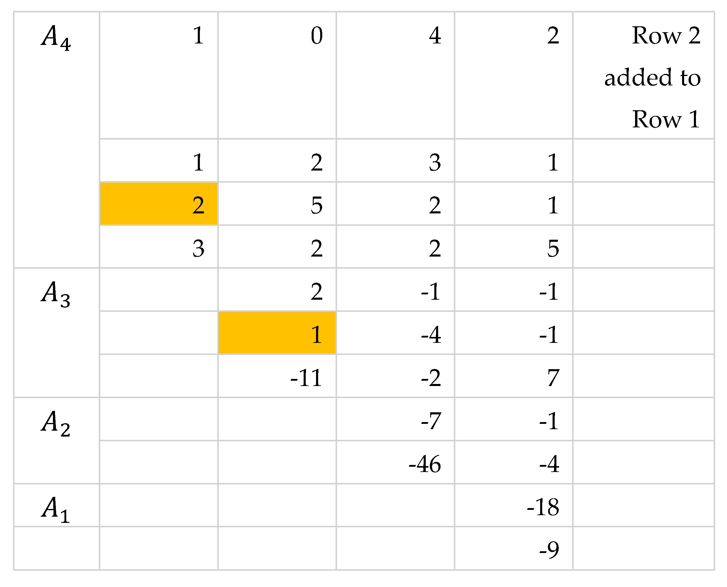
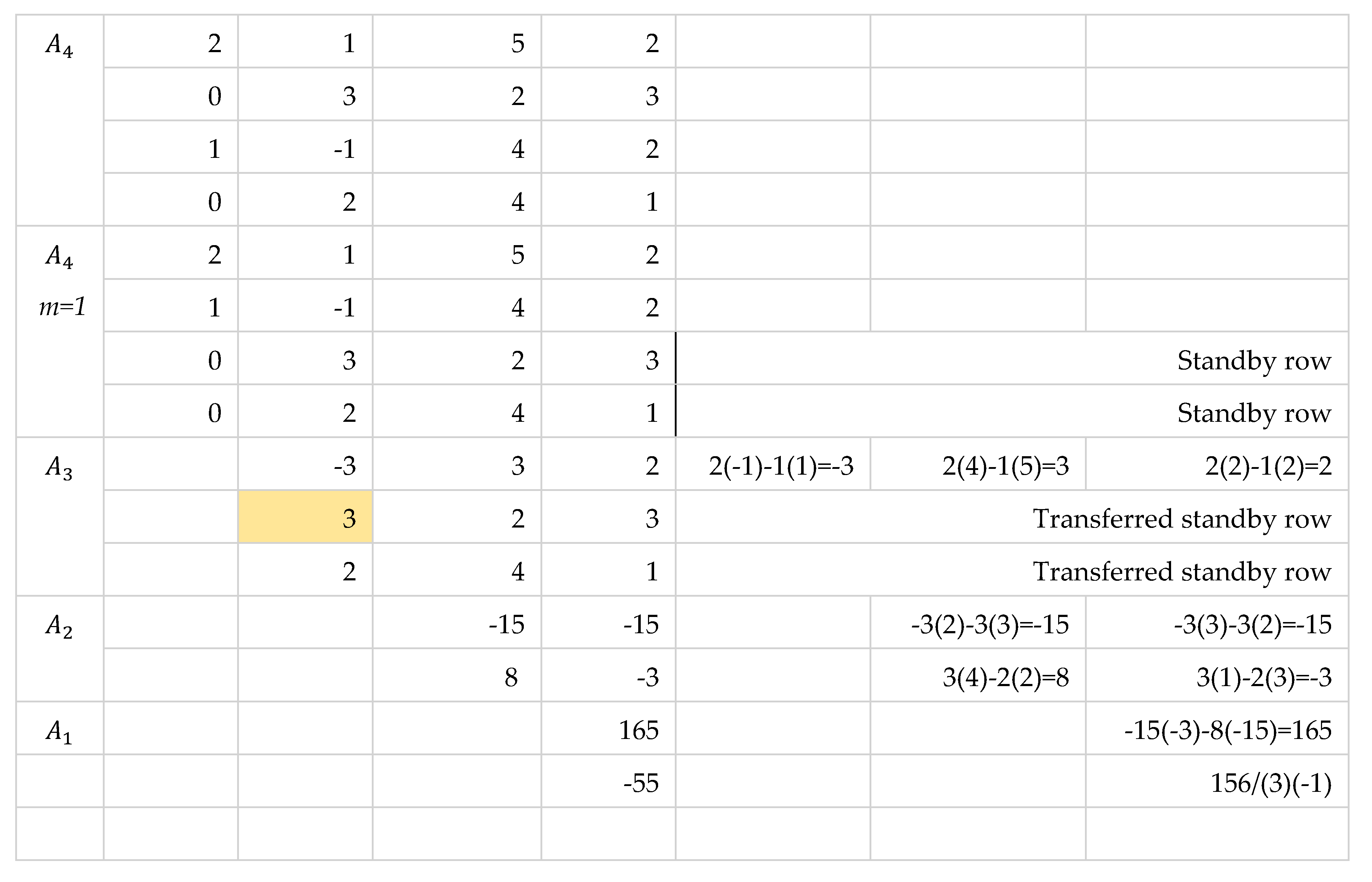
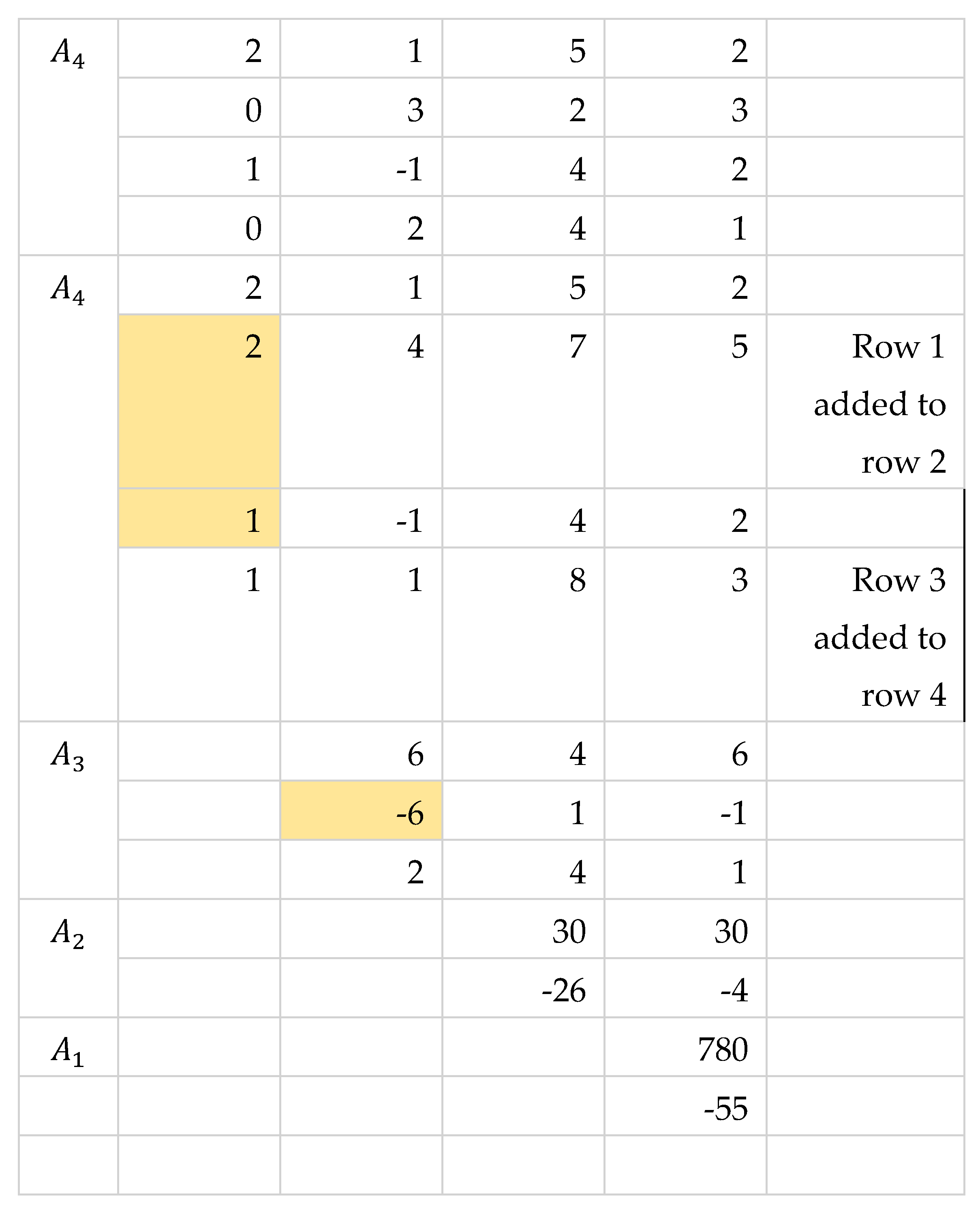
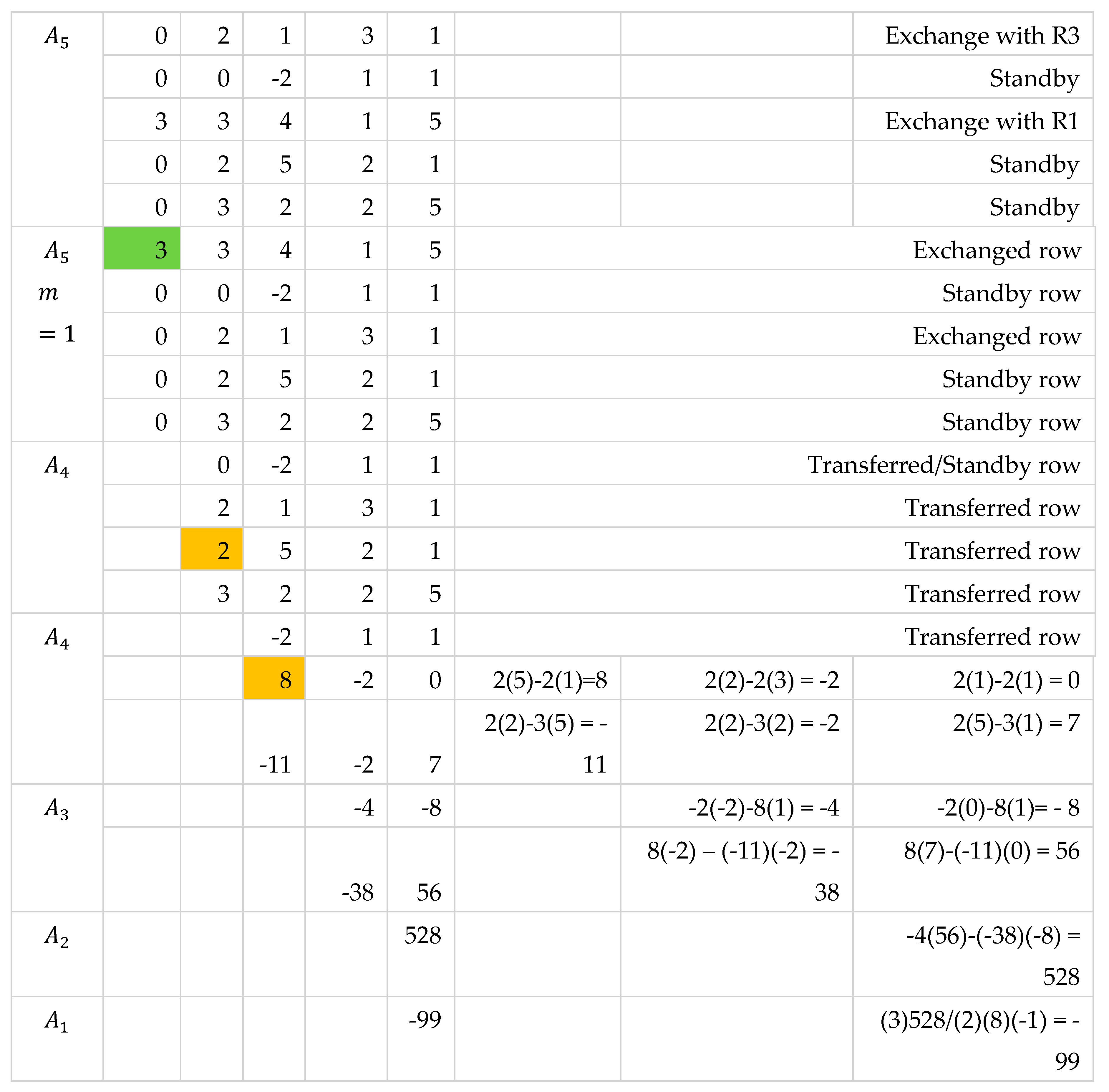
Appendix A

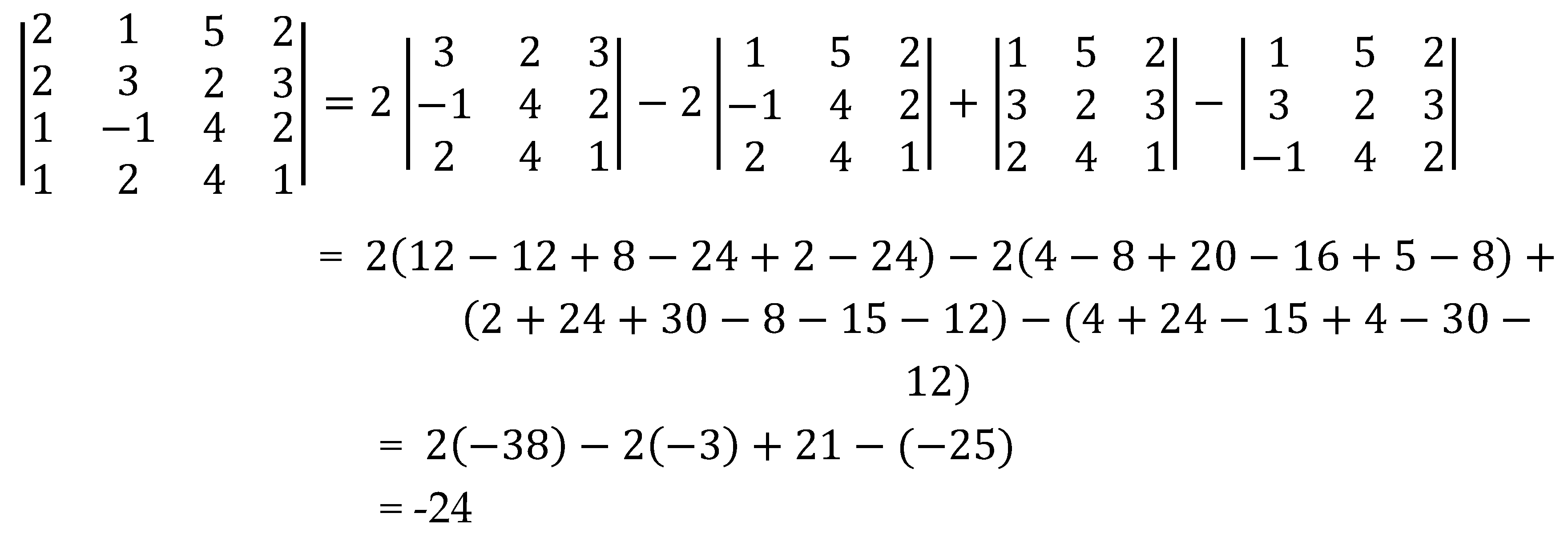
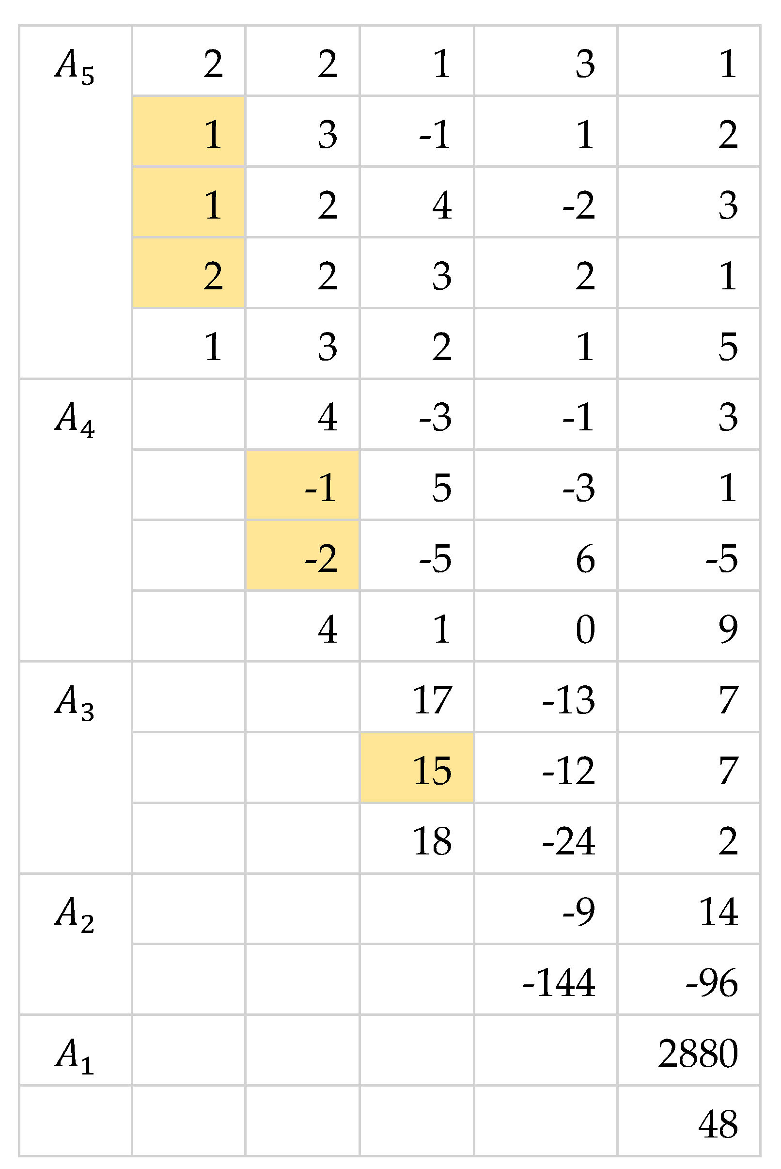
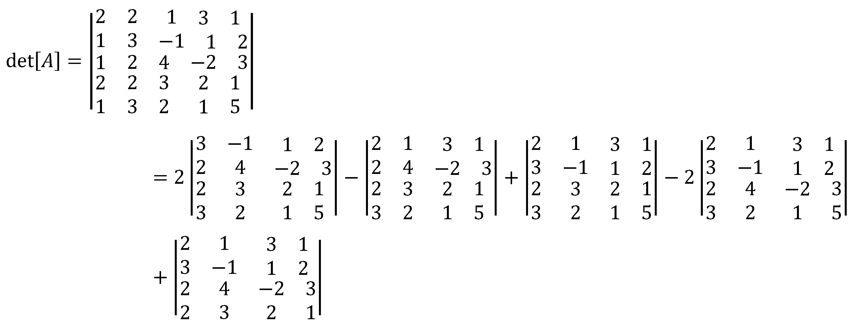
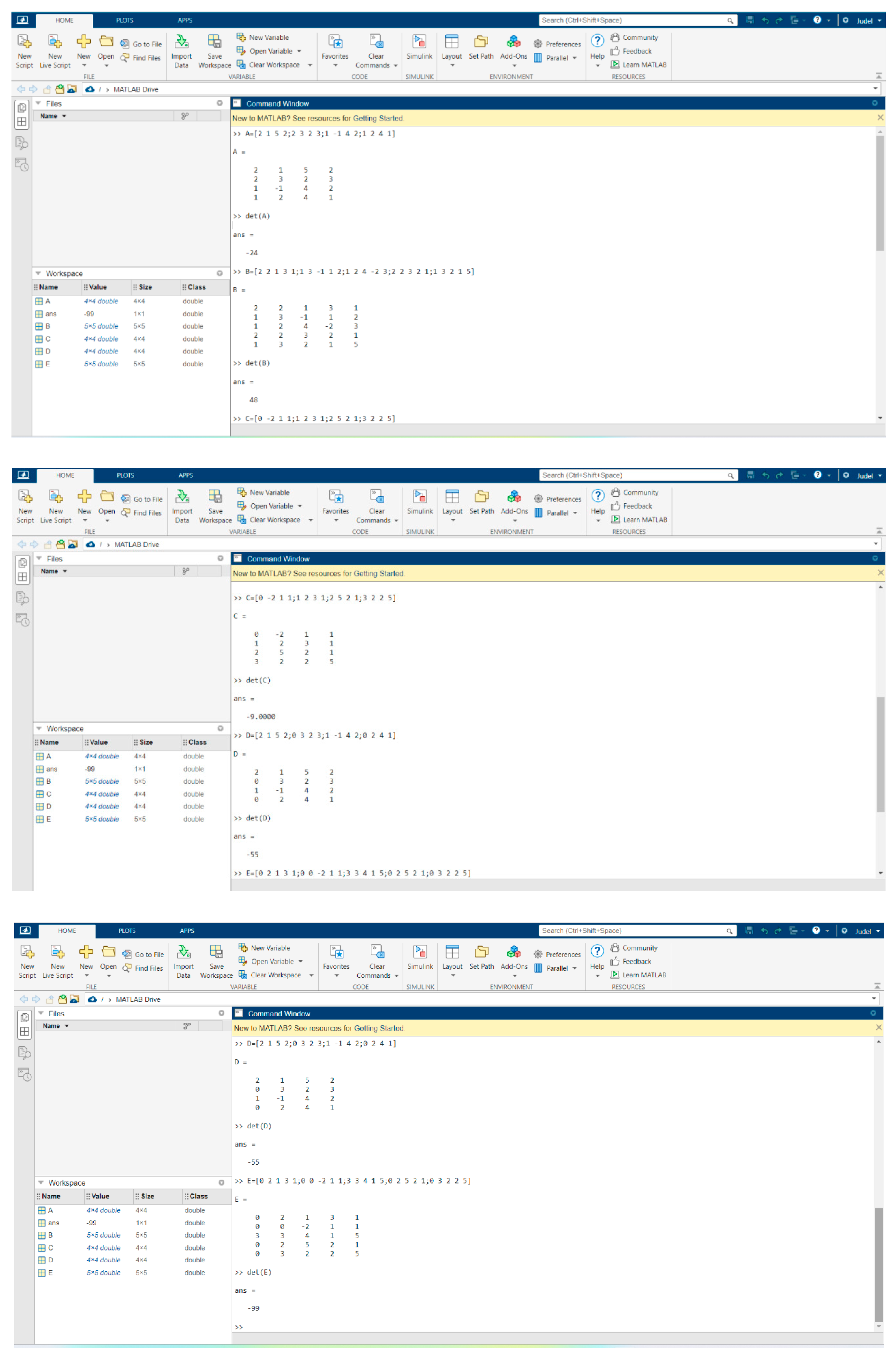
Experiments with Proposed Methods

We provide illustrative examples for the proposed methods and we verify the results using co-factor expansion and Matlab (See Appendix B).

Illustration 1.

4 \times 4

matrix All First Entries Are Non-zeros

A = [\begin{matrix} 2 & 2 & 5 & 2 \\ 2 & 3 & 2 & 3 \\ 1 & - 1 & 4 & 2 \\ 1 & 2 & 4 & 1 \end{matrix}]

Solution by cross-multiplication method.

Solution by co-factor expansion

We expand at the first column to get

Illustration 2.

5 \times 5

matrix All First Entries Are Non-zeros

A = [\begin{matrix} 2 & 2 & 1 & 3 & 1 \\ 1 & 3 & - 1 & 1 & 2 \\ 1 & 2 & 4 & - 2 & 3 \\ 2 & 2 & 3 & 2 & 1 \\ 1 & 3 & 2 & 1 & 5 \end{matrix}]

Computation of determinants by cross-multiplication method.

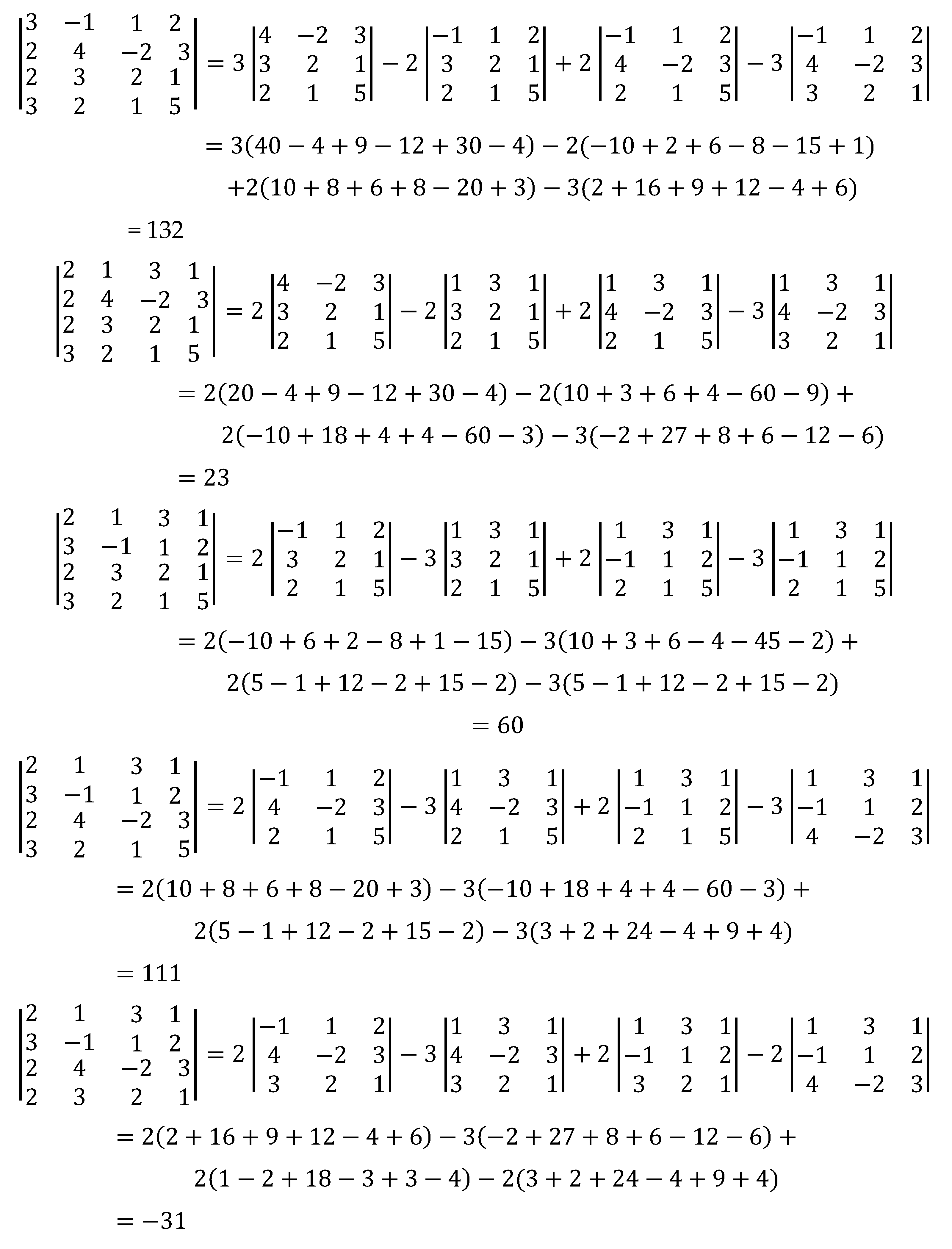
Verification of result by co-factor expansion.

We compute the determinant of each submatrix separately.

Thus,

\det [A] = 2 (132) - 23 + 60 - 2 (111) - 31 = 48

Illustration 3. First Entry of First or Last Row is Zero

C = [\begin{matrix} 0 & - 2 & 1 & 1 \\ 1 & 2 & 3 & 1 \\ 2 & 5 & 2 & 1 \\ 3 & 2 & 2 & 5 \end{matrix}]

The other approach is to add the row with zero first entry by another row with nonzero first entry.

Illustration 4. Some In-between First Entries are Zeros

D = [\begin{matrix} 2 & 1 & 5 & 2 \\ 0 & 3 & 2 & 3 \\ 1 & - 1 & 4 & 2 \\ 0 & 2 & 4 & 1 \end{matrix}]

We apply similar technique as in Illustration 2.

Illustration 5. Only One Row Has Non-zero First Entry

E = [\begin{matrix} 0 & 2 & 1 & 3 & 1 \\ 0 & 0 & - 2 & 1 & 1 \\ 3 & 3 & 4 & 1 & 5 \\ 0 & 2 & 5 & 2 & 1 \\ 0 & 3 & 2 & 2 & 5 \end{matrix}]

Appendix B

Matlab Generated Results

References

Kolman, B.; Hill, D. Elementary Linear Algebra with Applications 9^th Ed; Pearson Education Ltd.: London, UK, 2014. [Google Scholar]
Sobamowo, M. On the extension of Sarrus’. International Journal of Engineering Mathematics, 2016. [CrossRef]
Anton, H.; Rorres, C.; Kaul, A. Elementary Linear Algebra, 12th Ed. John Wiley and Sons: NY, USA, 2019.
Rice, A.; Torrence, E. ; Shutting up like a telescope: Lewis Carroll’s “Curious” Condensation Method for evaluating determinants. The College Mathematics Journal, 2007, 38, 85–95. [Google Scholar] [CrossRef]
Harwood, R. C.; Main, M.; Donor, M. An elementary proof of Dodgson's condensation method for calculating determinants" Faculty Publications - Department of Mathematics and Applied Science, 2016.
Seifullin, T. Computation of determinants, adjoint matrices, and characteristic polynomials without division. Cybernetics and Systems Analysis, 38, 2002.
Ji-Teng, J.; Wang, J.; He, Q.; Yu-Cong, Y. A division-free algorithm to numerically evaluating the determinant of a special quasi-tridiagonal matrix. Journal of Mathematical Chemistry, 60, 2022.
Bae, Y.; Lee, I. (2017). Determinant formulae of matrices with certain symmetry and its applications. Symmetry, 9, 2017.
Ji-Teng, J. A breakdown-free algorithm for computing the determinants of periodic tridiagonal matrices. Numerical Algorithm, 83, 2020.s.
Ji-Teng, J.; Yu-Cong, Y.; He, Q. A block diagonalization based algorithm for the determinants of block k-tridiagonal matrices. Journal of Mathematical Chemistry, 59, 2021.

Disclaimer/Publisher’s Note: The statements, opinions and data contained in all publications are solely those of the individual author(s) and contributor(s) and not of MDPI and/or the editor(s). MDPI and/or the editor(s) disclaim responsibility for any injury to people or property resulting from any ideas, methods, instructions or products referred to in the content.

© 2023 by the authors. Licensee MDPI, Basel, Switzerland. This article is an open access article distributed under the terms and conditions of the Creative Commons Attribution (CC BY) license (http://creativecommons.org/licenses/by/4.0/).

Copyright: This open access article is published under a Creative Commons CC BY 4.0 license, which permit the free download, distribution, and reuse, provided that the author and preprint are cited in any reuse.

MDPI Initiatives

Important Links

Choose an area of interest and we will send you notifications of new preprints at your preferred frequency.

Disclaimer

Computation of Matrix Determinants by Cross-Multiplication: A Rethinking of Dodgson’s Condensation and Reduction by Elementary Row Operations Methods

Abstract

1. Introduction

2. Development of Proposed Algorithm

3. Cross-Multiplication and Dodgson’s Condensation Method in 3 x 3 Matrices

4. Alternate Proof of Cross-Multiplication Method

5. Some Special Cases

6. Conclusions

Acknowledgments

Conflicts of Interest

Appendix A

Appendix B

References

MDPI Initiatives

Important Links

Subscribe