Preprint
Article

Pattern Formation in a Predator-Prey Model with Allee Effect and Hyperbolic Mortality on Multiplex Networks

Altmetrics

Downloads

107

Views

60

Comments

0

A peer-reviewed article of this preprint also exists.

Lei Shi  †,Jiaying Zhou  †,
Yong Ye  *

  † These authors contributed equally to this work.

This version is not peer-reviewed

Submitted:

26 June 2023

Posted:

27 June 2023

You are already at the latest version

Alerts
Abstract
With the rapid development of network science, Turing pattern on complex networks has attracted extensive attention from researchers. In this paper, we focus on spatial patterns in multiplex ER (Erdös-Rényi) random networks, taking the predator-prey model with Allee effect and hyperbolic mortality as an example. In theory, the threshold condition for generating Turing pattern is given using the Turing instability theory of multiplex networks. Numerically, we design relevant experiments to explore the impact of network topology on Turing pattern. The factors considered include model parameters, diffusion rate, average degree of the network, and differences in the average degree of different layers. The results indicate that the importance of diffusion rate and network average degree for Turing pattern is affirmed on the single-layer network. For multiplex networks, the differentiation of average degrees in different layers controls the generation of Turing pattern, which is not affected by the diffusion rates of the two populations. More interestingly, we observe the switching of Turing pattern and spatiotemporal pattern. We believe that these findings contribute to a better understanding of self-organization on complex networks.
Keywords: 
Subject: Computer Science and Mathematics  -   Mathematical and Computational Biology

MSC:  92D25; 35K57

1. Introduction

As early as around 1925, Lotka and Volterra proposed a mathematical model to describe the population evolution of snow rabbits (prey) and lynx (predators), known as the Lotka-Volterra model [1]. Since then, researchers have conducted in-depth research and improvement on the model based on real-life backgrounds [2,3,4,5,6,7,8,9,10,11,12]. What interests us is that in 2012, Nagano and Maeda introduced diffusion terms into the classical Rosenzweig-MacArthur model and analyzed the reaction-diffusion Rosenzweig-MacArthur model [3,13]. They provided a phase diagram of the model and studied its lattice formation, revealing the existence of various spatiotemporal patterns, including well-known spiral and lattice patterns. In 2014, Zhang et al. pointed out that the model did not have the possibility of generating Turing pattern based on this, so they attempted to consider more complex inducing factors such as hyperbolic mortality [4] or delay [14]. They also displayed many beautiful spatial patterns, including hexagonal spot patterns, stripe patterns, micro spirals patterns, and target patterns. Liu and his colleagues have long been engaged in the study of the Allee effect on population model dynamics [5,6,7,8,11,12]. Therefore, in 2019, they attempted to introduce the predator-prey model with hyperbolic mortality proposed by Zhang et al. into the Allee effect. The study found that the Allee effect would increase the independence of pattern, in other words, it would make the spatial distribution of the population more concentrated, which is beneficial for the continuation of the population [7]. In 2010, the Turing pattern on large-scale random networks was first studied by Nakao and Mikhailov, and their findings demonstrated that early linear instability caused network nodes to naturally separate into wealthy and poor groups. In the following nonlinear stage, the freshly forming Turing pattern undergoes yet another significant reshaping. Several steady-state coexistence and hysteresis effects were observed [2]. Inspired by this, the work on Turing pattern diagrams on complex networks has been widely carried out, and these works can be subdivided into others from the perspective of theory and application background. In theory, it mainly focuses on the development of different types of network pattern formation theory and pattern dynamics [15,16,17,18,19,20,21,22,23,24,25]. In application, it mainly focuses on different research backgrounds, such as infectious disease models, population models, and rumor propagation models [26,27,28,29,30,31,32,33,34,35,36,37,38,39,40,41,42,43,44,45,46,47,48,49]. Here, we choose the population model as the research background. In particular, we will describe in detail the work related to Turing pattern based on predator-prey models in complex networks. In 2012, Fernandes and collaborators generalized the work of Nakao and Mikhailov to food web models, and their results highlighted that differences in abundance distribution among patches could be dynamically generated through a self-organized Turing pattern [26]. Subsequently, in 2019 and 2021, Chang et al. considered the small delay and large delay factors in the Leslie-Gower model, respectively. The aim was to explore the evolution of rich spatiotemporal patterns caused by delay and further confirmed the impact of delay on Turing pattern [27,32]. Meanwhile, Liu et al. tested the Leslie-Gower model in LA4 ( 2 D lattices with average degrees k = 4 ) network, LA12 network ( 2 D lattices with average degrees k = 12 ), LA23 network ( 2 D lattices with average degrees k = 23 ), ER random network [50] and BA (Barabási-Albert) scale-free network [51] in 2020, respectively. And found that the average degree of the network plays an important role in the pattern formation [31]. Influenced by the above works, Ye and Zhou constructed a predator-prey model with Allee effect and hyperbolic mortality on ER random network, and discovered the existence of the spatiotemporal pattern affected by the initial value [52]. Their model expression is as follows
d u i d t = α ¯ u i 1 u i u i u i + A α ¯ u i v i 1 + β u i + d 1 j = 1 N L i j u j , d v i d t = β u i v i 1 + β u i γ v i 2 e + η v i + d 2 j = 1 N L i j v j , u i ( 0 ) 0 , v i ( 0 ) 0 .
The biological significance of each parameter and variable in model (1) is shown in Table 1 and [3,4,7,52].
Table 1. Notation used in model (1).
Parameter Description
u i The prey population occupies every node index i in the network
v i The predator population occupies every node index i in the network
d 1 The self-diffusion rate of prey population
d 2 The self-diffusion rate of predator population
α ¯ The ratio of intrinsic growth rate to predator birth rate
A The weak Allee effect constant
β The ratio of environmental capacity to half-saturation prey density
e The coefficients of light attenuation by water
η The coefficients of light attenuation by self-shading
γ The death rate of the predator population
L i j The elements in the network Laplacian matrix L
The above work is mostly based on single-layer networks. We note that generating Turing pattern on multiplex networks does not seem to require significant differences in diffusion rates between two populations, which was first mentioned in [17]. Therefore, compared to single-layer networks, multiplex networks are more general. Soon after, in 2020, Gao et al. attempted to consider cross-diffusion mechanisms on multiplex networks and found many complex heterogeneous spatial patterns that had not yet been discovered in single-layer networks [28]. They applied it to the predator-prey model in 2023 and also discovered these complex heterogeneous spatial patterns, which effectively confirmed their early findings [48]. To our knowledge, most of the research on patterns in multiplex networks currently focuses on Turing pattern, while other types of spatiotemporal patterns are rarely mentioned. Therefore, this article takes the predator-prey model with Allee effect and hyperbolic mortality as an example to explore the possibility of spatial patterns on multiplex networks. Therefore, model (1) is rewritten as follows
d u i d t = f u i , v i + d 1 j = 1 N L i j ( u ) u j , d v i d t = g u i , v i + d 2 j = 1 N L i j ( v ) v j , u i ( 0 ) 0 , v i ( 0 ) 0 .
The reaction term here can be expressed as
f ( u i , v i ) = α ¯ u i ( 1 u i ) u i u i + A α ¯ u i v i 1 + β u i , g ( u i , v i ) = β u i v i 1 + β u i γ v i 2 e + η v i .
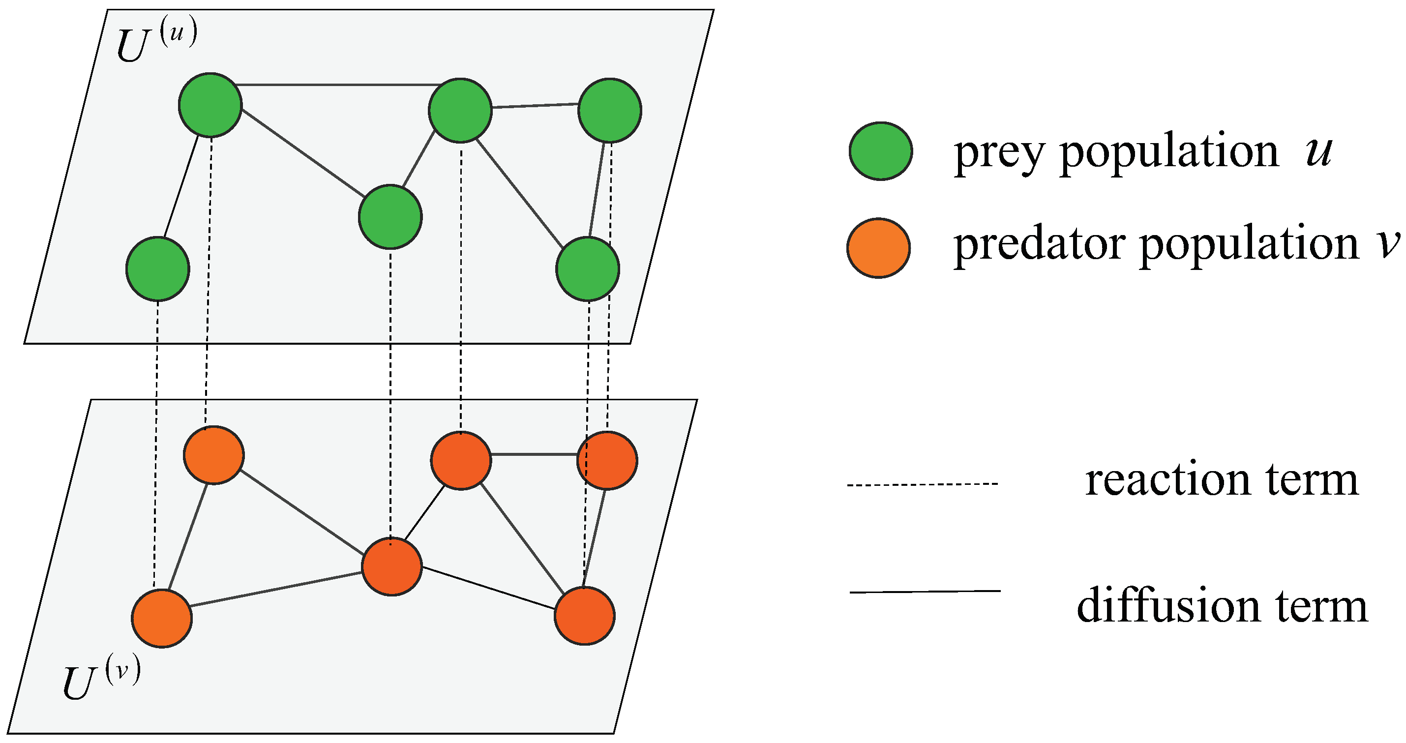
We divide the population on the multiplex ER random networks into two categories: prey population u i and predator population v i . The schematic diagram is shown in Figure 1. The prey population u i and predator population v i occupy every node in layers U ( u ) and U ( v ) , respectively. There is an interactive relationship between two populations across the layers through the imaginary lines which means the reaction term f u i , v i and g u i , v i . Meanwhile, species on the network will also flow in or out of this node on their own layer through the solid lines which means the diffusion term d 1 j = 1 N L i j ( u ) u j and d 2 j = 1 N L i j ( v ) v j .
Figure 1. Reaction-diffusion prey-predator model locates in a multiplex ER random network, which shows the prey population u i (green nodes) and predator population v i (orange nodes) occupy every node on U ( u ) layer and U ( v ) layer, respectively. Among them, the imaginary lines represent the reaction term, and the solid lines represent the diffusion term.
Preprints 77662 g001
Here, the total number of nodes in the network is N, and its topology is defined as a symmetric adjacency matrix whose elements satisfy A i j = 1 if the node i and j are connected where i , j = 1 , , N and i j , otherwise A i j = 0 . We set the degree of node i as shown by k i = j = 1 N A i j . In addition, we sort network nodes index i in decreasing order of their degrees k i . The aim is to ensure that k 1 k 2 k N is established [2,17]. The sum of the incoming fluxes from other connecting nodes index j to node index i provides the diffusion of species u and v at the node index i. Fick’s law states that the flux is inversely proportional to the difference in node concentrations. So, the network Laplacian matrix L i j = A i j k i δ i j is considered and δ i j illustrates the Kronecker product, the diffusive flux of the predator population v to the node index i is written as j = 1 N L i j ( v ) v j and the diffusive flux of the prey population u to the node index i as j = 1 N L i j ( u ) u j . The biological significance of other parameters is shown in Table 1.
The main structure of this paper can be organized as follows. In Section 2, by utilizing the Turing instability theory on multiplex networks, the threshold conditions for Turing bifurcation were calculated. In Section 3, numerical experiments are carried out on Turing pattern in single-layer networks and multiplex networks, respectively. In Section 4, numerical experiments are carried out on spatiotemporal patterns in single-layer networks and multiplex networks, respectively. In Section 5, a brief conclusion is given.

2. Turing instability on multiplex networks

In this section, we mainly focus on the critical conditions for the occurrence of Turing bifurcation in model (2). Just as the prerequisite for Turing instability in continuous media is to ensure that the positive equilibrium is stable without diffusion. Therefore, on the networks, we need to first determine the stability of the positive equilibrium of the non-diffusion model (2). For the convenience of calculation, we set η = γ and e = 1 as in [4,7,52]. According to [52], model (2) may have four equilibria E 0 = ( 0 , 0 ) , E 1 = ( 1 , 0 ) , E * ( 1 ) = ( u * ( 1 ) , v * ( 1 ) ) , and E * ( 2 ) = ( u * ( 2 ) , v * ( 2 ) ) when β > γ 1 γ , 0 < γ < 1 , and γ β < A < ( β γ γ β ) 2 + 4 β γ 2 4 β 2 γ . It should be emphasized that u * ( 1 ) = β γ γ β ( β γ γ β ) 2 + 4 ( γ β A ) β γ 2 β γ , u * ( 2 ) = β γ γ β + ( β γ γ β ) 2 + 4 ( γ β A ) β γ 2 β γ , and v * ( i ) = β γ u * ( i ) with i = 1 , 2 . Furthermore, we can obtain the following lemma.
Lemma 1.
[52] When β > γ 1 γ , 0 < γ < 1 , and γ β < A < ( β γ γ β ) 2 + 4 β γ 2 4 β 2 γ , the stability conditions for the two positive equilibra in model (2) can be summarized as follows
  • The positive equilibrium E * ( 1 ) is always unstable which is a saddle.
  • Let H = v * ( 2 ) 1 + β u * ( 2 ) u * ( 2 ) v * ( 2 ) 1 + β u * 2 1 u * ( 2 ) + A v * ( 2 ) 1 + β u * ( 2 ) A + u * ( 2 ) v * ( 2 ) 1 + β u * ( 2 ) 2 > 0 , which can be obtained α ¯ H = β u * ( 2 ) H 1 + β u * ( 2 ) 2 . So we have the following conclusion: if α ¯ < α ¯ H , then E * ( 2 ) is stable. If α ¯ > α ¯ H , then E * ( 2 ) is unstable. Particularly, when α ¯ = α ¯ H Hopf bifurcation occurs since d Tr d α ¯ = H > 0 and
    Tr = α ¯ H v * ( 2 ) 1 + β u * ( 2 ) u * ( 2 ) v * ( 2 ) 1 + β u * ( 2 ) 1 u * ( 2 ) + A v * ( 2 ) 1 + β u * ( 2 ) A + u * ( 2 ) v * ( 2 ) 1 + β u * ( 2 ) 2 β u * ( 2 ) 1 + β u * ( 2 ) 2 .
When applied to classical continuous media, the non-uniform perturbation is typically decomposed as spatial Fourier modes that correspond to various wave numbers for plane waves. Inspired by this, Othmer and Scriven observed that the eigenvectors can indicate the influence of the plane wave and wave number on the network, which is Φ ( α ) = ϕ 1 ( α ) , , ϕ N ( α ) and eigenvalues Λ α ( u , v ) ( α = 1 , , N ) of Laplace matrix, where j = 1 N L i j ( u , v ) ϕ j ( α ) = Λ α ( u , v ) ϕ i ( α ) [53]. Refer to [2], the following condition 0 = Λ 1 ( u , v ) Λ 2 ( u , v ) Λ N ( u , v ) need to be satisfied. The eigenvectors are orthonormalized as i = 1 N ϕ i ( α ) ϕ i ( ω ) = δ α , ω and α , ω = 1 , , N . The small perturbations δ u i and δ v i are introduced to the positive equilibrium like u i , v i = ( u * ( 2 ) , v * ( 2 ) ) + δ u i , δ v i and the linearizing form of model (2) can be written as
d δ u i d t = a 11 δ u i + a 12 δ v i + d 1 j = 1 N L i j ( u ) δ u j , d δ v i d t = a 21 δ u i + a 22 δ v i + d 2 j = 1 N L i j ( v ) δ v j ,
where
a 11 = α ¯ v * ( 2 ) 1 + β u * ( 2 ) α ¯ u * ( 2 ) v * ( 2 ) 1 + β u * ( 2 ) 1 u * ( 2 ) + α ¯ A v * ( 2 ) 1 + β u * ( 2 ) A + u * ( 2 ) α ¯ v * ( 2 ) 1 + β u * ( 2 ) 2 ,
a 12 = α ¯ u * ( 2 ) 1 + β u * ( 2 ) , a 21 = β 2 v * ( 2 ) 1 + β u * ( 2 ) 2 , a 22 = β u * ( 2 ) 1 + β u * ( 2 ) 2 .
In particular, for a single-layer network, where Λ α ( u ) = Λ α ( v ) = Λ α . A detailed analysis can be seen in [52], which can be summarized as the following lemma. In addition, to have an intuitive feeling, we give the dispersion relation between Laplace eigenvalue ( Λ α ) and model (2) eigenvalue ( λ α ) in Figure 3 and Figure 5.
Lemma 2.
[52] There are two critical values a 11 + a 22 = 0 and a 11 a 22 a 12 b 21 + a 11 d 2 Λ α + a 22 d 1 Λ α + d 1 d 2 Λ α 2 = 0 . They correspond to the critical value conditions for generating Hopf bifurcation and Turing bifurcation, respectively. And we can determine Λ α ( 1 ) and Λ α ( 2 ) as
Λ α ( 1 ) = a 11 d 2 + a 22 d 1 Δ 2 d 1 d 2 , Λ α ( 2 ) = a 11 d 2 + a 22 d 1 + Δ 2 d 1 d 2 .
Where Δ = a 11 d 2 + a 22 d 1 2 4 d 1 d 2 a 11 a 22 a 12 a 21 , Turing instability requires Λ α ( 1 ) < Λ α < Λ α ( 2 ) to be maintained.
Next, we consider the more general case of multiplex networks, whose Turing-instability conditions are derived from [17]. We rewrite the linearized model (3) as follows
d S d t = ( R + D ) S ,
where S = δ u 1 , , δ u N , δ v 1 , , δ v N T is considered as the perturbation vector and
R = a 11 I N a 12 I N a 21 I N a 22 I N , D = d 1 L ( u ) 0 0 d 2 L ( v ) .
Notice that I N = diag ( 1 , 1 , , 1 ) be used as N × N identity matrix, L ( u ) and L ( v ) are the Laplacian matrix of U ( u ) layer and U ( v ) layer, respectively. Among them, D = A D is established, here
A = d 1 A ( u ) 0 0 d 2 A ( v ) , D = d 1 D ( u ) 0 0 d 2 D ( v ) .
Specifically, A ( u ) and A ( v ) are the adjacency matrices of U ( u ) layer and U ( v ) layer, respectively. The D ( u ) and D ( v ) represent the degree matrices of U ( u ) layer and U ( v ) layer, respectively. For the matrices A , which has elements with values of order O d 1 or O d 2 . For the matrices D , which has elements with values of order O d 1 k ( u ) or O d 2 k ( v ) . Assuming U ( u ) layer and U ( v ) layer are dense enough that k ( u ) 1 and k ( v ) 1 . According to [17], it is easy to see that A can be neglected and D D . Therefore, Eq. (4) can be rewritten as
d S d t = a 11 I N d 1 D ( u ) a 12 I N a 21 I N a 22 I N d 2 D ( u ) S .
It is not difficult to obtain
Det a 11 d 1 k ( u ) λ a 12 a 21 a 22 d 2 k ( u ) λ = 0 ,
where k ( u ) and k ( v ) represent the degrees of nodes in U ( u ) layer and U ( v ) layer, respectively. In summary, the characteristic equation can be expressed as
λ 2 Tr k ( u ) , k ( v ) λ + Det k ( u ) , k ( v ) = 0 ,
where
Tr k ( u ) , k ( v ) = a 11 + a 22 ( d 1 k ( u ) + d 2 k ( v ) ) , Det k ( u ) , k ( v ) = a 11 a 22 a 12 a 21 ( a 11 d 2 k ( v ) + a 22 d 1 k ( u ) ) + d 1 d 2 k ( u ) k ( v ) .
Therefore, we have the following discussion, if Tr k ( u ) , k ( v ) < 0 and Det k ( u ) , k ( v ) < 0 , Turing instability will occur. When E * ( 2 ) = u * ( 2 ) , v * ( 2 ) is stable in non-diffusion model (2). Obviously, the condition of Tr k ( u ) , k ( v ) < 0 holds because of k ( u ) 0 and k ( v ) 0 . Consequently, Turing instability need Det k ( u ) , k ( v ) < 0 is established, that is to say
k ( u ) > a 11 a 22 a 12 a 21 a 11 d 2 k ( u ) a 22 d 1 d 1 d 2 k ( v )
for a 22 d 1 d 1 d 2 k ( v ) > 0 or
k ( u ) < a 11 a 22 a 12 a 21 a 11 d 2 k ( u ) a 22 d 1 d 1 d 2 k ( v )
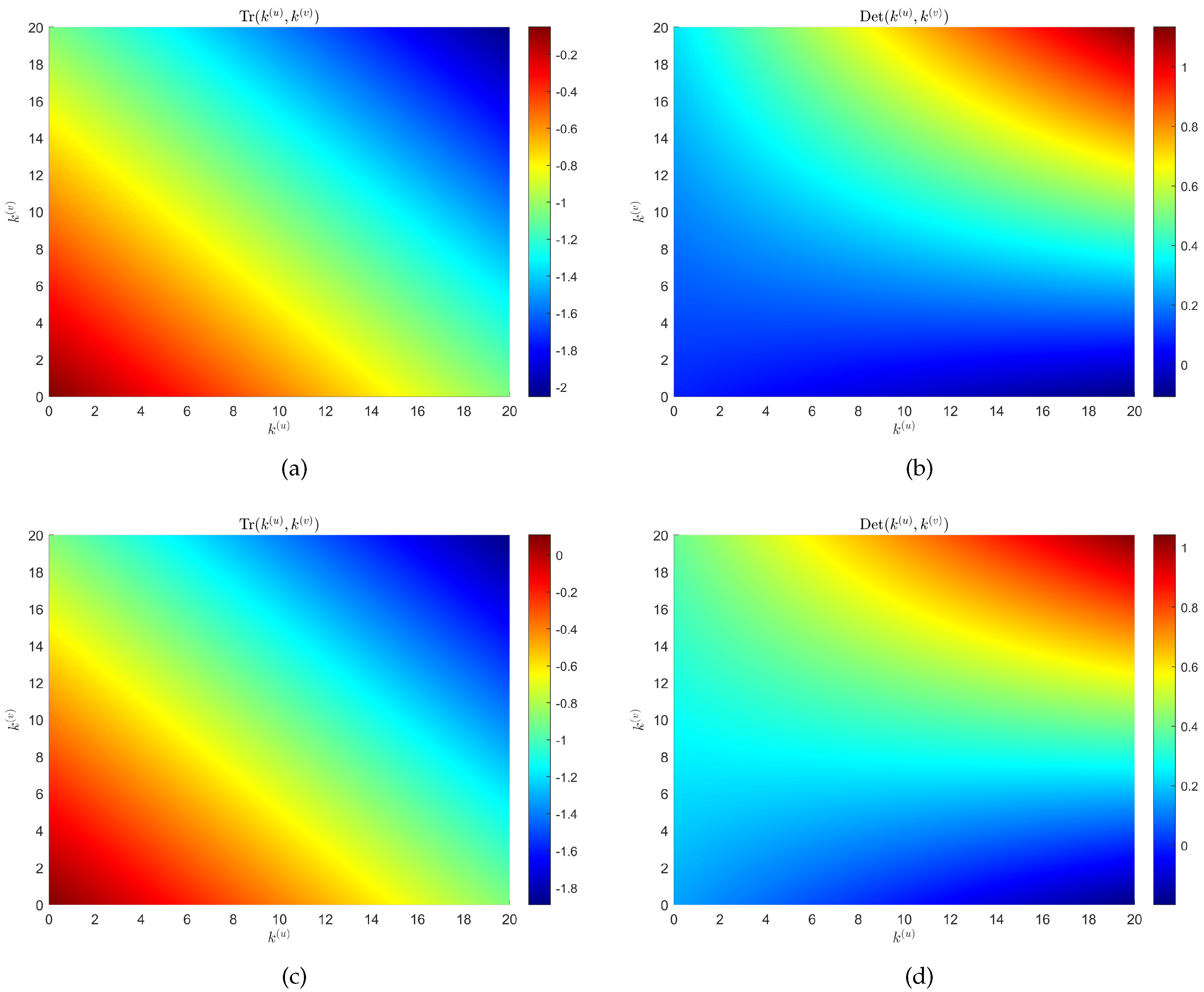
for a 22 d 1 d 1 d 2 k ( v ) < 0 . Similar to the idea of a single-layer network, we give the relationship between Tr k ( u ) , k ( v ) and Det k ( u ) , k ( v ) with the degrees of nodes in U ( u ) layer and U ( v ) layer ( k ( u ) , k ( v ) ) , respectively (see Figure 2). We can find that when the control parameter α ¯ = 1.2 , there is the possibility of Tr k ( u ) , k ( v ) > 0 . That is to say, when the diffusion item is considered, model (2) becomes unstable. Note that it is a non-Turing pattern at this time.
Figure 2. When α ¯ = 0.65 , panels (a) and (b) represent the relationship between Tr k ( u ) , k ( v ) and Det k ( u ) , k ( v ) with the degrees of nodes in U ( u ) layer and U ( v ) layer ( k ( u ) , k ( v ) ) , respectively. When α ¯ = 1.2 , panels (a) and (b) represent the relationship between Tr k ( u ) , k ( v ) and Det k ( u ) , k ( v ) with the degrees of nodes in U ( u ) layer and U ( v ) layer ( k ( u ) , k ( v ) ) , respectively. The rest of the parameters are d 1 = 0.05 , d 2 = 0.05 , A = 0.01 , β = 6 , γ = 0.5 , e = 1 , and η = 0.5 .
Preprints 77662 g002

3. Turing pattern on networks

In this section, we discuss the evolution of Turing pattern on single-layer ER random networks and multiplex ER random networks. In particular, we take the predator diffusion rate d 2 , the average degree of the network Λ α , and the ratio of average degrees on different networks as the research objects, respectively. The purpose is to study the factors affecting the Turing pattern on the ER random network and discuss how these factors affect the generation of the pattern. Before starting the numerical experiment, we need to emphasize some basic settings, where the total number of nodes in the network is N = 1600 , the initial value is u i ( 0 ) = u * ( 2 ) + 0.1 × rand ( 0 , 1 ) , v i ( 0 ) = v * ( 2 ) + 0.1 × rand ( 0 , 1 ) , and the remaining parameters are d 1 = 0.05 , A = 0.01 , α ¯ = 0.65 , β = 6 , γ = 0.5 , e = 1 , η = 0.5 , where rand ( 0 , 1 ) is a random perturbation. u * ( 2 ) = u * and v * ( 2 ) = v * always holds in all figures.

3.1. Diffusion rate induces Turing pattern on single-layer network
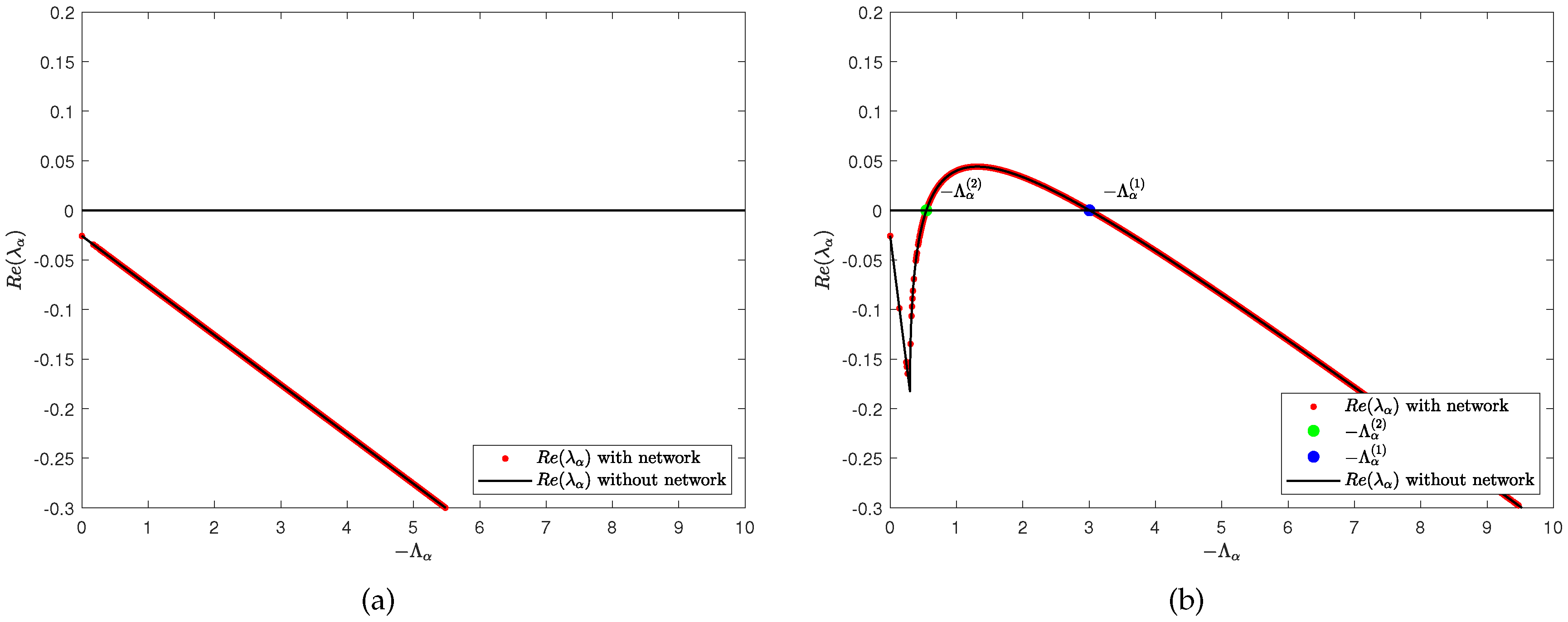
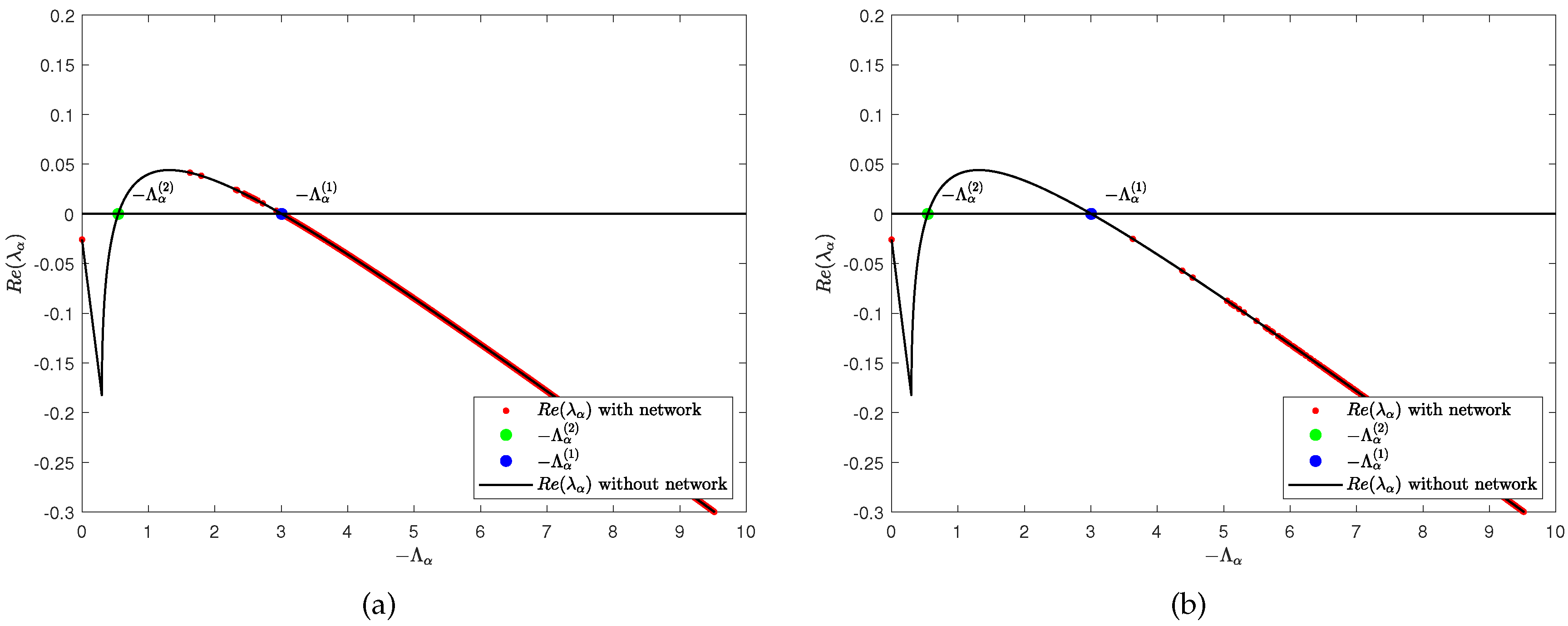
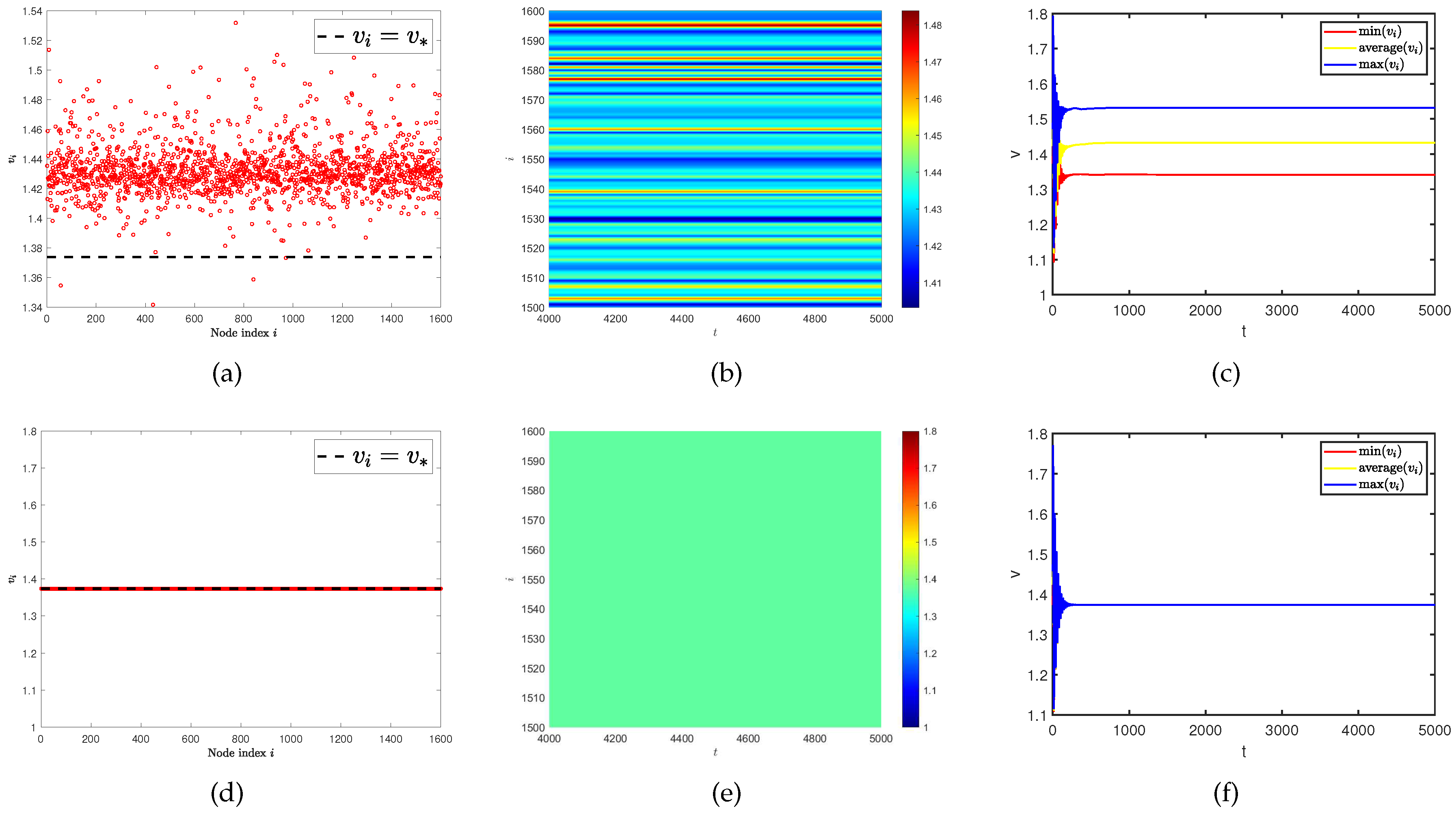
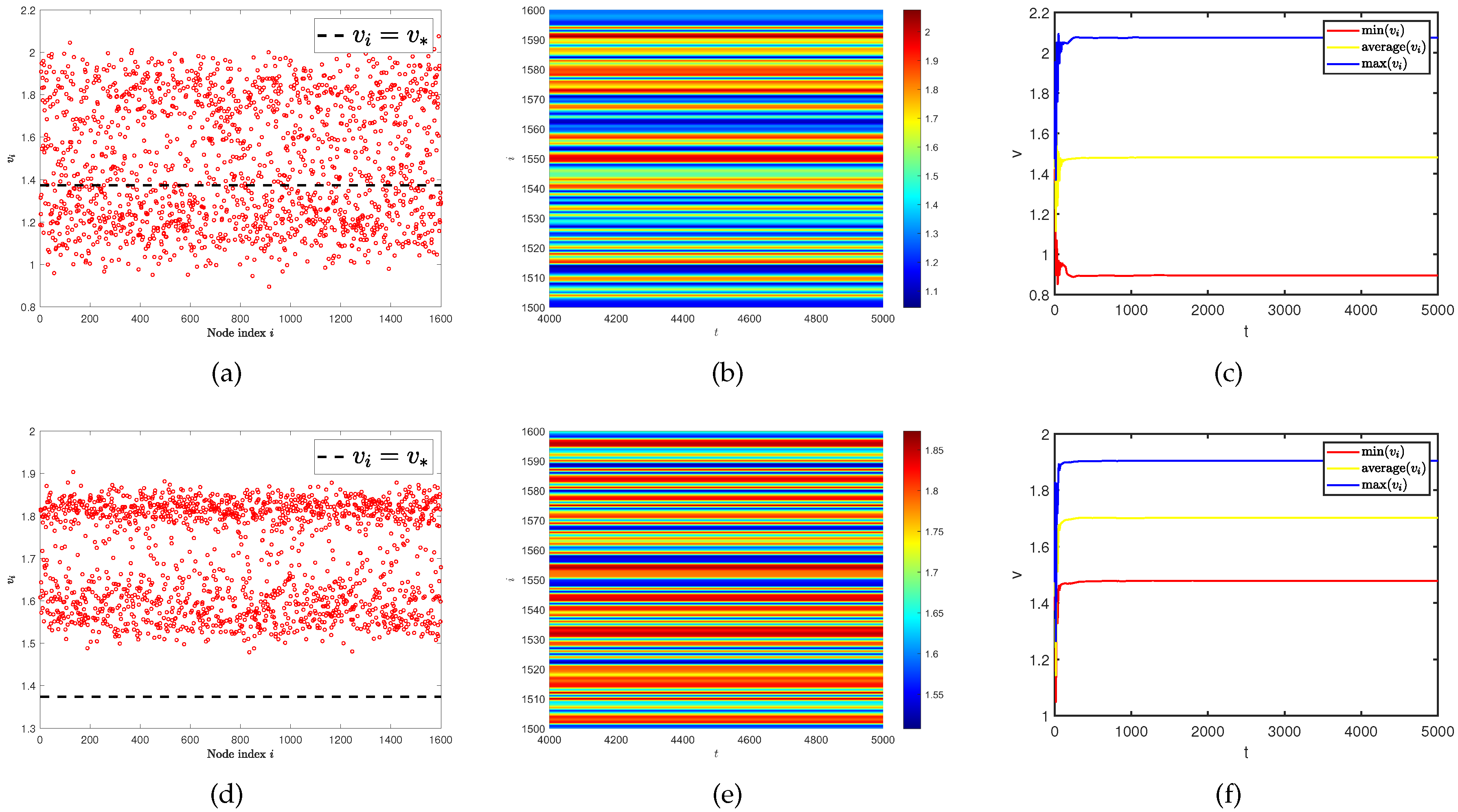
We first discuss the effect of predator diffusion rate d 2 on Turing pattern. According to Lemma 2, we give the dispersion relation between Laplace eigenvalue ( Λ α ) and model (2) eigenvalue ( λ α ) as shown in Figure 3. It can be seen that when the two populations have the same diffusion rate ( d 1 = d 2 = 0.05 ), there is no Λ α so that R e ( λ α ) > 0 . However, when we increase the predator diffusion rate ( d 2 = 1 ), there are critical thresholds Λ α ( 1 ) 3.01 and Λ α ( 2 ) 0.546 such that R e ( λ α ) = 0 . Therefore, it is not difficult to see that when Λ α ( Λ α ( 1 ) , Λ α ( 2 ) ) , Turing instability occurs where R e ( λ α ) > 0 . In addition, we also provide the density (red dots) of predator population ( v i ) with different predator diffusion rates, the predator population density ( v i ) on the ER random network varies with time under different predator diffusion rates, and the curves of the maximum, minimum, and average values of the predator population density ( v i ) in all nodes on the network at different predator diffusion rates over time, respectively (see Figure 4). The results indicate that on single-layer network, the diffusion rate plays a decisive role in Turing pattern.
Figure 3. Dispersion relation between Laplace eigenvalue ( Λ α ) and model (2) eigenvalue ( λ α ) with different diffusion rate. The predator diffusion rate is d 2 = 0.05 for (a). The predator diffusion rate is d 2 = 1 for (b). Where the average degree is k ( u ) = k ( v ) = 4 . The rest of the parameters are d 1 = 0.05 , A = 0.01 , α ¯ = 0.65 , β = 6 , γ = 0.5 , e = 1 , and η = 0.5 .
Preprints 77662 g003
Figure 4. (a) and (d) represent the density (red dots) of predator population ( v i ) with different predator diffusion rates. (b) and (e) represent the predator population density ( v i ) on the ER random network varies with time under different predator diffusion rates. (c) and (f) represent the curves of the maximum, minimum, and average values of the predator population density ( v i ) in all nodes on the network at different predator diffusion rates over time. The predator diffusion rate is d 2 = 0.05 for (a), (b), and (c). The predator diffusion rate is d 2 = 1 for (d), (e), and (f). Where the average degree is k ( u ) = k ( v ) = 4 .
Preprints 77662 g004

3.2. Network average degree induces Turing pattern on single-layer network
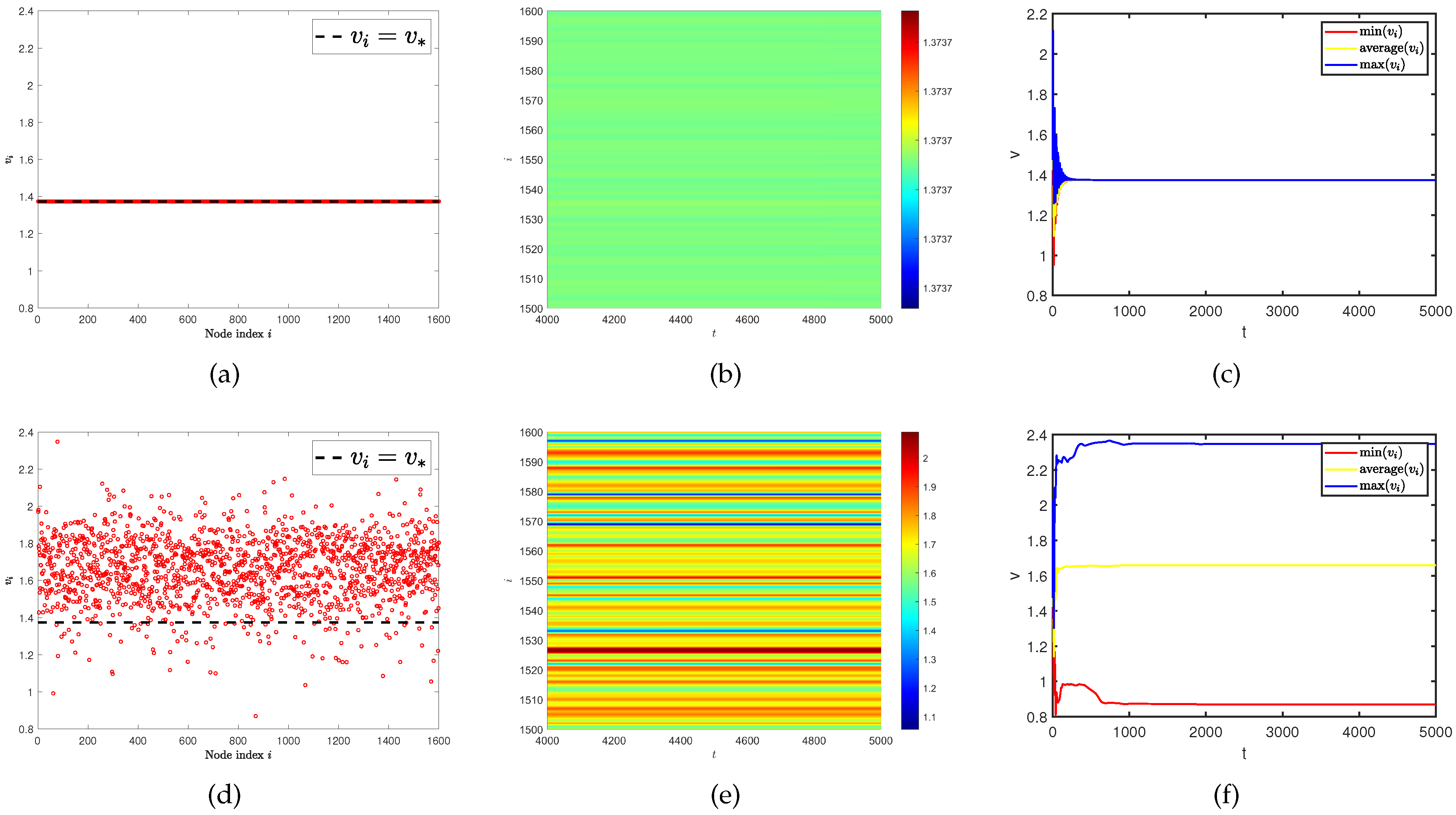
The above experiments have well verified the importance of diffusion rate. In this group of experiments, we investigate how the spatial distribution of species changes when the diffusion rate meets the Turing instability condition and changes the average degree of the network ( k = k ( u ) = k ( v ) ). As we gradually increase the value of the average degree of the network k , we find that although the Turing instability region always exists, the eigenvalues Λ α (red dots) of the Laplacian matrix do not fall within this region. Therefore, when k = k ( u ) = k ( v ) = 15 , Turing pattern is not captured in Figure 5. Similarly, in this set of experiments, we also provide the density (red dots) of predator population ( v i ) with different network average degrees, predator population density ( v i ) on the ER random network varies with time under different network average degrees, and curves of the maximum, minimum, and average values of the predator population density ( v i ) in all nodes on the network at different average degrees over time (see Figure 6). The results indicate that as the average degree of the network increases, the spatial distribution of species gradually concentrates at equilibrium E * ( 2 ) = ( u * ( 2 ) , v * ( 2 ) ) until the Turing pattern disappears.
Figure 5. Dispersion relation between Laplace eigenvalue ( Λ α ) and model (2) eigenvalue ( λ α ) with different average degree. The average degree is k ( u ) = k ( v ) = 10 for (a). The average degree is k ( u ) = k ( v ) = 15 for (b). The rest of the parameters are d 1 = 0.05 , d 2 = 0.05 , A = 0.01 , α ¯ = 0.65 , β = 6 , γ = 0.5 , e = 1 , and η = 0.5 .
Preprints 77662 g005
Figure 6. (a) and (d) represent the density (red dots) of predator population ( v i ) with different network average degrees. (b) and (e) represent the predator population density ( v i ) on the ER random network varies with time under different network average degrees. (c) and (f) represent the curves of the maximum, minimum, and average values of the predator population density ( v i ) in all nodes on the network at different average degrees over time. The average degree is k ( u ) = k ( v ) = 10 for (a), (b), and (c). The average degree is k ( u ) = k ( v ) = 15 for (d), (e), and (f).
Preprints 77662 g006

3.3. Ratio of network average degree induces Turing pattern on multiplex networks

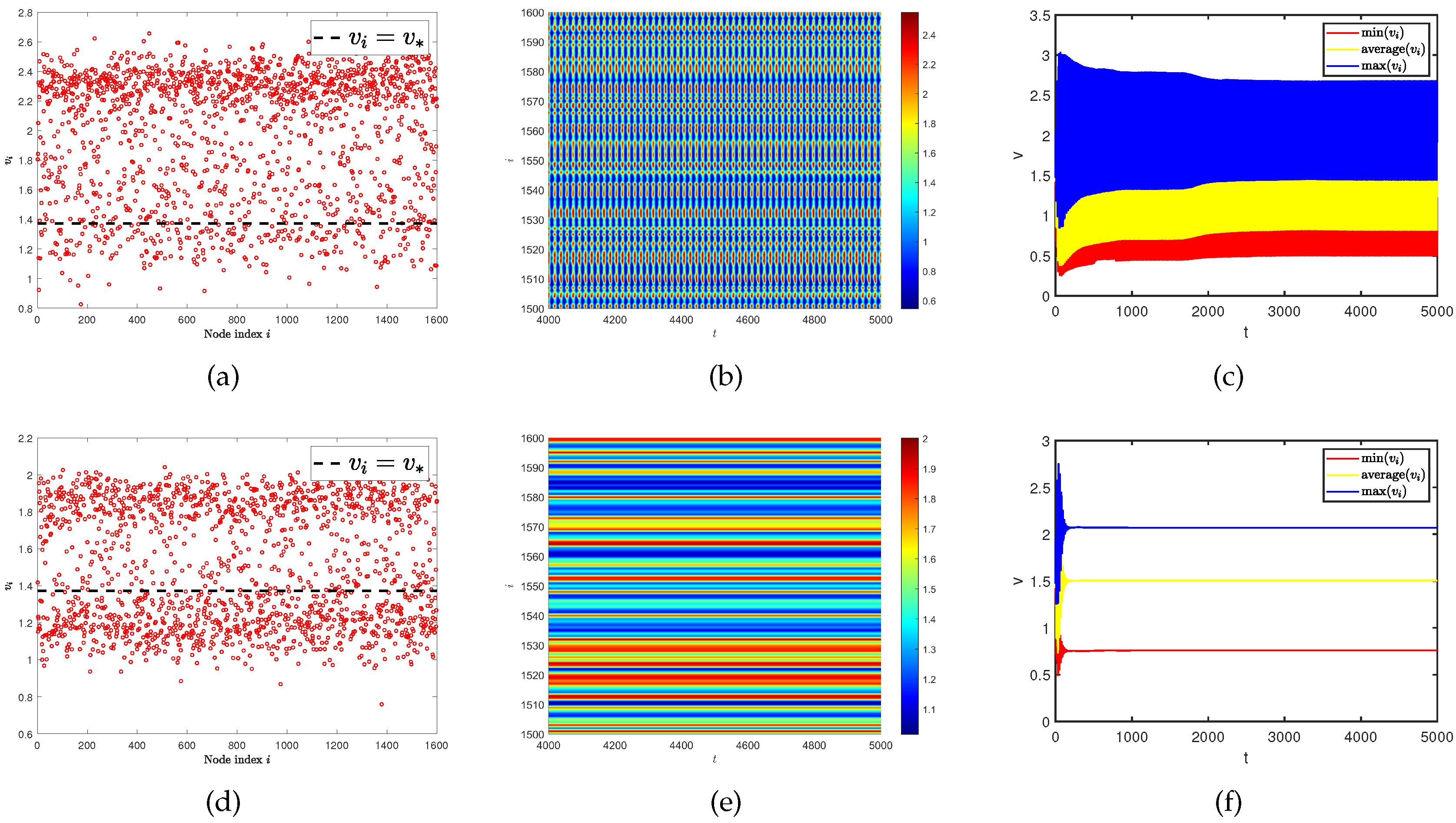
It is well known that diffusivity plays a decisive role in the formation of Turing pattern on continuous media, but is it the same on discrete media or complex networks? Kouvaris et al. provide an answer to this in their work, stating that even if two populations have the same diffusion rate on multiplex networks, Turing pattern will be generated [17]. Therefore, we hope to verify whether this conclusion is equally applicable to our model. Before starting the experiment, we set the diffusion rate of the two populations to d 1 = d 2 = 0.05 and determine the average degree k ( u ) = 4 on U ( u ) layer. Observing the changes in the spatial distribution pattern of species by changing the average degree k ( v ) on U ( v ) layer. The threshold conditions for generating Turing bifurcation can be obtained from Eq. (8) and (9), as shown in Figure 7. It is not difficult to find that the Turing instability condition does not hold when the average degree of the two layers network is the same ( k ( u ) = k ( v ) = 4 ). So, we increase the average degree on U ( v ) layer, which led to Turing instability. By comparing Figure 4((d), (e), and (f)) and Figure 8, it can be intuitively seen that the Turing pattern has evolved from scratch. In addition, we also find that the spatial distribution of species changes with the increase of average degree differentiation in different layers.
Figure 7. (a), (b), and (c) represent degree combination for pairs of nodes in plane k ( v ) k ( u ) together with the curve of Turing bifurcation (black) on multiplex ER random networks. The average degree on U ( v ) layer is k ( v ) = 4 , k ( v ) = 20 , and k ( v ) = 80 for (a), (b), and (c). Where have same average degree on U ( u ) layer k ( u ) = 4 .
Preprints 77662 g007
Figure 8. (a) and (d) represent the density (red dots) of predator population ( v i ) with different ratios of network average degree. (b) and (e) represent the predator population density ( v i ) on the ER random network varies with time under different ratios of network average degree. (c) and (f) represent the curves of the maximum, minimum, and average values for the predator population density ( v i ) in all nodes on the network over time. The average degree on U ( u ) layer and U ( v ) layer are k ( u ) = 4 and k ( v ) = 20 for (a), (b), and (c). The average degree on U ( u ) layer and U ( v ) layer are k ( u ) = 4 and k ( v ) = 80 for (d), (e), and (f).
Preprints 77662 g008

4. Spatiotemporal pattern on networks

When we theoretically analyze the Turing instability on the network, we find that the premise of Turing pattern always requires that the positive equilibrium in the non-diffusion model is always stable. If the positive equilibrium in the non-diffusion model is not stable at this time, what kind of spatial distribution state will the model present? On continuous media, Nagano and Maeda discovered the existence of spiral and lattice patterns [3]. What will happen on ER random network? It should be pointed out that this spatial pattern type is not Turing pattern but another spatiotemporal pattern. So, we conduct the following numerical experiments. The value of the parameter is the same as Section 3, except for α .

4.1. Parameter induces spatiotemporal pattern on single-layer network
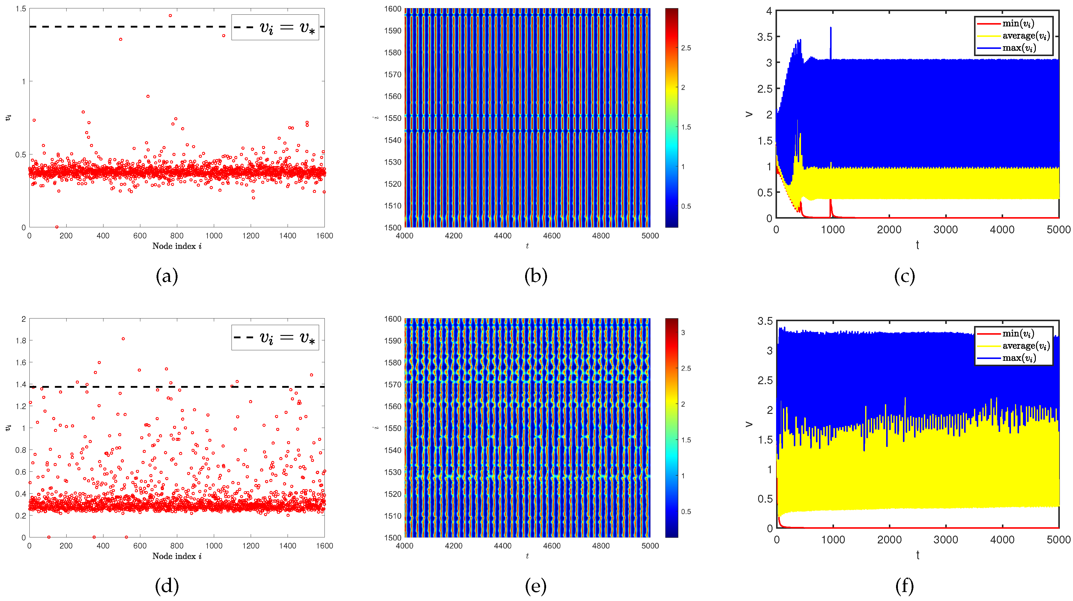
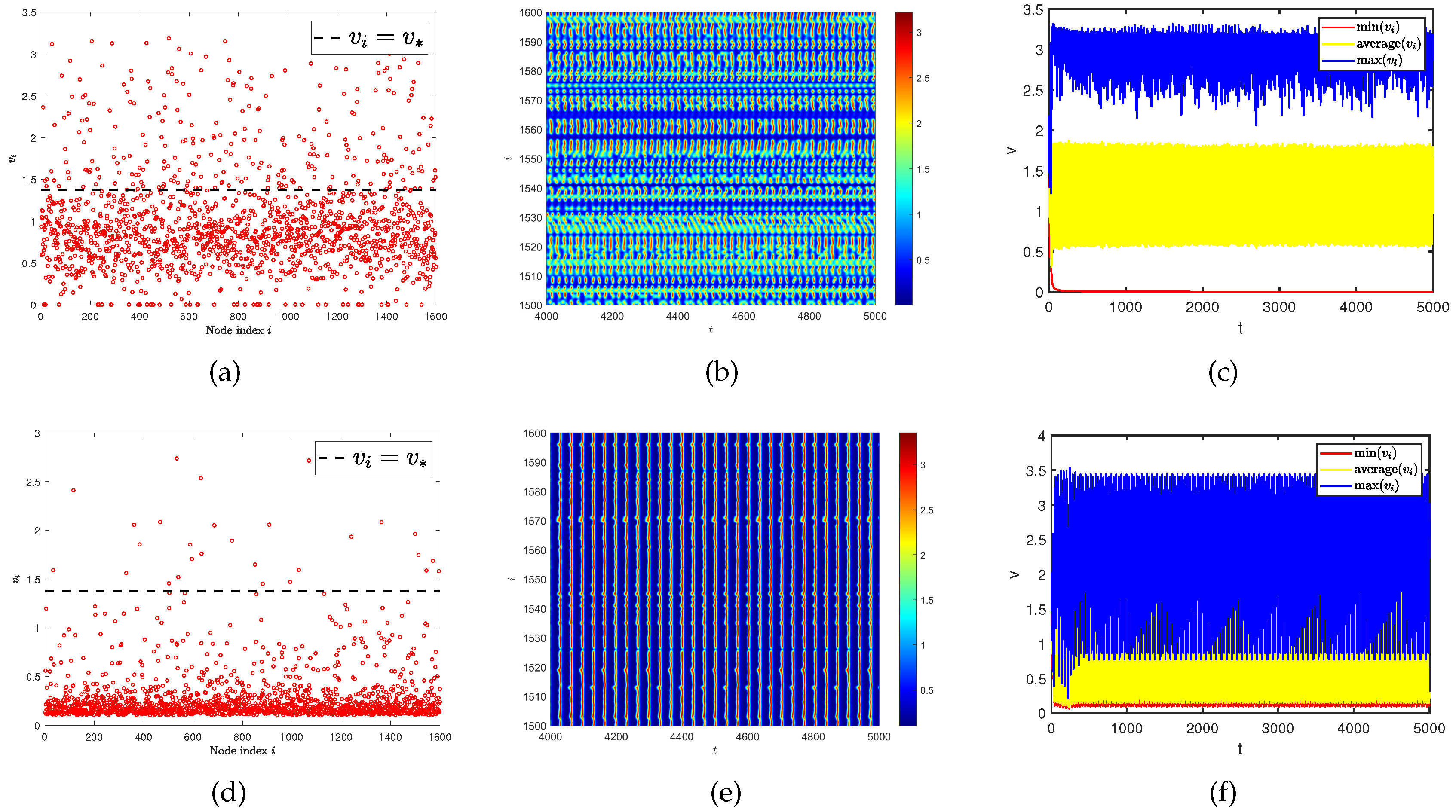
In the beginning, we hope to conduct our testing on single-layer network and by changing the value of control parameter α ¯ . It turned out that even if the diffusion rates of two populations are the same, we could still discover the existence of spatial heterogeneity patterns in Figure 9. And as α ¯ increases, this phenomenon becomes more apparent. However, when looking at Figure 4 (a), (b), and (c), no such spatiotemporal patterns are observed. So we speculate that this is a spatiotemporal pattern phenomenon caused by parameters. By observing the curves of the maximum, minimum, and average values of the predator population density ( v i ) in all nodes on the network at different parameters α ¯ over time. We find the existence of an obvious irregular periodic oscillation phenomenon. Similar spatiotemporal pattern phenomena have also received attention in some work [40,41,42].
Figure 9. (a) and (d) represent the density (red dots) of predator population ( v i ) with different parameters α . (b) and (e) represent the density of the predator population ( v i ) on the ER random network varies with time under different parameters α ¯ . (c) and (f) represent the curves of the maximum, minimum, and average values of the predator population density ( v i ) in all nodes on the network at different parameters α ¯ over time. The parameter is α ¯ = 0.85 for (a), (b), and (c). The parameter is α ¯ = 1.2 for (d), (e), and (f). Where the average degree is k ( u ) = k ( v ) = 4 and same diffusion rate is d 1 = d 2 = 0.05 .
Preprints 77662 g009

4.2. Network average degree induces spatiotemporal pattern on single-layer network and multiplex networks
Then, we consider whether this spatiotemporal pattern is still affected by the average degree of single-layer network and multiplex networks. Therefore, we provide a comparative experiment of spatiotemporal patterns under different average degrees (see Figure 10). When the average degree is k ( u ) = k ( v ) = 2 , spatial heterogeneity is particularly evident. If the diffusion rates of two populations on the single-layer network are the same, there will not be Turing pattern generated. We want to know what changes occur if the generation conditions of Turing pattern and spatiotemporal pattern are generated simultaneously. Due to this issue, we conduct our experiment on multiplex networks. To our surprise, we find that as the average value on the controlled U ( v ) layer increased (from k ( v ) = 13 to k ( v ) = 20 ), the two spatial patterns switched as shown in Figure 11. In other words, the spatiotemporal pattern transforms into Turing pattern, and even the oscillations in time disappear and become stable. These results indicate that network topology also has a significant impact on the generation of spatiotemporal patterns.
Figure 10. (a) and (d) represent the density (red dots) of predator population ( v i ) with different network average degrees. (b) and (e) represent the predator population density ( v i ) on the ER random network varies with time under different network average degrees. (c) and (f) represent the curves of the maximum, minimum, and average values of the predator population density ( v i ) in all nodes on the network at different average degrees over time. The average degree is k ( u ) = k ( v ) = 2 for (a), (b), and (c). The average degree is k ( u ) = k ( v ) = 5 for (d), (e), and (f). Where have the same diffusion rate d 1 = d 2 = 0.05 and α ¯ = 1.2 .
Preprints 77662 g010
Figure 11. (a) and (d) represent the density (red dots) of predator population ( v i ) with different ratios of network average degree. (b) and (e) represent the predator population density ( v i ) on the ER random network varies with time under different ratios of network average degree. (c) and (f) represent the curves of the maximum, minimum, and average values for the predator population density ( v i ) in all nodes on the network over time. The average degree on U ( u ) layer and U ( v ) layer are k ( u ) = 4 and k ( v ) = 13 for (a), (b), and (c). The average degree on U ( u ) layer and U ( v ) layer are k ( u ) = 4 and k ( v ) = 20 for (d), (e), and (f). Where have the same diffusion rate d 1 = d 2 = 0.05 and α ¯ = 1.2 .
Preprints 77662 g011

5. Conclusion

Taken together, this paper considers the spatial patterns of a predator-prey model with weak Allee effect and hyperbolic mortality on multiplex networks. The main content of our research is to theoretically analyze the critical conditions for generating Turing patterns on multiplex networks. Moreover, we also conduct numerical experiments on several factors that affect spatial patterns, such as diffusion rate, the average degree of network, and the ratio of average degree. Our results indicate that the diffusion rate of two populations is not a necessary condition for generating Turing pattern on multiplex networks, which effectively validates the conclusion of [17,54]. More interestingly, we also found a switch between two types of spatial patterns. Specifically, when model (2) exhibits spatiotemporal patterns under specific parameters, as the difference in the average degree of the different layers on the network increases, the pattern transforms into Turing pattern. Meanwhile, this phenomenon seems to be unique to multiplex networks and has not been found on single-layer networks. These findings once again emphasize the important impact of network topology on species spatial distribution.
In future work, we will continue our work from two aspects: (1) The practical significance of spatiotemporal patterns in biological systems often represents the spatial distribution of species. In recent years, there have been some control methods for Turing patterns in reaction-diffusion systems on networks, which can effectively present the spatial distribution of species in a predetermined pattern [33,34,35]. Therefore, we hope to apply this theory to our model. (2) The higher-order structure of networks has gradually become a new research hotspot in the field of network science. Considering that higher-order interactions affect the topological properties of the network, which can interfere with the formation of spatiotemporal patterns [25,47,54]. Therefore, we also hope to introduce higher-order networks into our model, to understand the potential role of higher-order structures in species spatial distribution.

Author Contributions

Conceptualization, Y.Y. and J.Z.; methodology, L.S.; software, J.Z.; validation, L.S., J.Z., and Y.Y.; formal analysis, L.S.; writing—original draft preparation, L.S. and J.Z.; writing—review and editing, Y.Y.; supervision, Y.Y.; project administration, L.S.; funding acquisition, L.S. All authors have read and agreed to the published version of the manuscript.

Funding

Lei Shi acknowledges support by the Lanzhou Jiaotong University 2022 doctoral research start-up fee (No. 1520020961).

Data Availability Statement

Not applicable.

Acknowledgments

The authors would like to thank the reviewers for the helpful comments, which improved the presentation of this paper.

Conflicts of Interest

The authors declare that there are no conflict of interest.

References

  1. Murray, J.D. Mathematical biology: I. An introduction; Springer, 2002. [Google Scholar] [CrossRef]
  2. Nakao, H.; Mikhailov, A.S. Turing patterns in network-organized activator–inhibitor systems. Nature Physics 2010, 6, 544–550. [Google Scholar] [CrossRef]
  3. Nagano, S.; Maeda, Y. Phase transitions in predator-prey systems. Physical Review E 2012, 85, 011915. [Google Scholar] [CrossRef] [PubMed]
  4. Zhang, T.; Xing, Y.; Zang, H.; Han, M. Spatio-temporal dynamics of a reaction-diffusion system for a predator–prey model with hyperbolic mortality. Nonlinear Dynamics 2014, 78, 265–277. [Google Scholar] [CrossRef]
  5. Shi, L.; Liu, H.; Wei, Y.; Ma, M.; Ye, J. The permanence and periodic solution of a competitive system with infinite delay, feedback control, and Allee effect. Advances in Difference Equations 2018, 2018, 400. [Google Scholar] [CrossRef]
  6. Ye, Y.; Liu, H.; Wei, Y.; Zhang, K.; Ma, M.; Ye, J. Dynamic study of a predator-prey model with Allee effect and Holling type-I functional response. Advances in Difference Equations 2019, 2019, 1–15. [Google Scholar] [CrossRef]
  7. Liu, H.; Ye, Y.; Wei, Y.; Ma, W.; Ma, M.; Zhang, K. Pattern formation in a reaction-diffusion predator-prey model with weak Allee effect and delay. Complexity 2019, 2019, 6282958. [Google Scholar] [CrossRef]
  8. Ye, Y.; Liu, H.; Wei, Y.m.; Ma, M.; Zhang, K. Dynamic study of a predator-prey model with weak Allee effect and delay. Advances in Mathematical Physics 2019, 2019, 7296461. [Google Scholar] [CrossRef]
  9. Ye, Y.; Zhao, Y. Bifurcation analysis of a delay-induced predator–prey model with Allee effect and prey group defense. International Journal of Bifurcation and Chaos 2021, 31, 2150158. [Google Scholar] [CrossRef]
  10. Ye, Y.; Zhao, Y.; Zhou, J. Promotion of cooperation mechanism on the stability of delay-induced host-generalist parasitoid model. Chaos, Solitons & Fractals 2022, 165, 112882. [Google Scholar] [CrossRef]
  11. Li, D.; Liu, H.; Han, X.; Lin, X.; Wei, Y. Stability and Bifurcation Analysis of Bazykin’s Model with Holling I Functional Response and Allee Effect. International Journal of Bifurcation and Chaos 2022, 32, 2250248. [Google Scholar] [CrossRef]
  12. Li, D.; Liu, H.; Zhang, H.; Ma, M.; Ye, Y.; Wei, Y. Bifurcation Analysis in a Predator-Prey Model with an Allee Effect and a Delayed Mechanism. Acta Mathematica Scientia 2023, 43, 1415–1438. [Google Scholar] [CrossRef]
  13. Rosenzweig, M.L.; MacArthur, R.H. Graphical representation and stability conditions of predator-prey interactions. The American Naturalist 1963, 97, 209–223. [Google Scholar] [CrossRef]
  14. Zhang, T.; Zang, H. Delay-induced Turing instability in reaction-diffusion equations. Physical Review E 2014, 90, 052908. [Google Scholar] [CrossRef] [PubMed]
  15. Asllani, M.; Challenger, J.D.; Pavone, F.S.; Sacconi, L.; Fanelli, D. The theory of pattern formation on directed networks. Nature communications 2014, 5, 1–9. [Google Scholar] [CrossRef] [PubMed]
  16. Asllani, M.; Busiello, D.M.; Carletti, T.; Fanelli, D.; Planchon, G. Turing patterns in multiplex networks. Physical Review E 2014, 90, 042814. [Google Scholar] [CrossRef]
  17. Kouvaris, N.E.; Hata, S.; Guilera, A.D. Pattern formation in multiplex networks. Scientific reports 2015, 5, 1–9. [Google Scholar] [CrossRef]
  18. Petit, J.; Asllani, M.; Fanelli, D.; Lauwens, B.; Carletti, T. Pattern formation in a two-component reaction–diffusion system with delayed processes on a network. Physica A: Statistical Mechanics and its Applications 2016, 462, 230–249. [Google Scholar] [CrossRef]
  19. Petit, J.; Lauwens, B.; Fanelli, D.; Carletti, T. Theory of Turing patterns on time varying networks. Physical review letters 2017, 119, 148301. [Google Scholar] [CrossRef]
  20. Tian, C.; Ruan, S. Pattern formation and synchronism in an allelopathic plankton model with delay in a network. SIAM Journal on Applied Dynamical Systems 2019, 18, 531–557. [Google Scholar] [CrossRef]
  21. Muolo, R.; Asllani, M.; Fanelli, D.; Maini, P.K.; Carletti, T. Patterns of non-normality in networked systems. Journal of theoretical biology 2019, 480, 81–91. [Google Scholar] [CrossRef]
  22. Liu, Z.; Tian, C. A weighted networked SIRS epidemic model. Journal of Differential Equations 2020, 269, 10995–11019. [Google Scholar] [CrossRef]
  23. Liu, Z.; Tian, C.; Ruan, S. On a network model of two competitors with applications to the invasion and competition of Aedes albopictus and Aedes aegypti mosquitoes in the United States. SIAM Journal on Applied Mathematics 2020, 80, 929–950. [Google Scholar] [CrossRef]
  24. Tian, C.; Liu, Z.; Ruan, S. Asymptotic and transient dynamics of SEIR epidemic models on weighted networks. European Journal of Applied Mathematics 2022, 1–24. [Google Scholar] [CrossRef]
  25. Muolo, R.; Gallo, L.; Latora, V.; Frasca, M.; Carletti, T. Turing patterns in systems with high-order interactions. Chaos, Solitons & Fractals 2023, 166, 112912. [Google Scholar] [CrossRef]
  26. Fernandes, L.D.; De Aguiar, M. Turing patterns and apparent competition in predator-prey food webs on networks. Physical Review E 2012, 86, 056203. [Google Scholar] [CrossRef] [PubMed]
  27. Chang, L.; Liu, C.; Sun, G.; Wang, Z.; Jin, Z. Delay-induced patterns in a predator–prey model on complex networks with diffusion. New Journal of Physics 2019, 21, 073035. [Google Scholar] [CrossRef]
  28. Gao, S.; Chang, L.; Wang, X.; Liu, C.; Li, X.; Wang, Z. Cross-diffusion on multiplex networks. New Journal of Physics 2020, 22, 053047. [Google Scholar] [CrossRef]
  29. Gan, W.; Zhu, P.; Liu, Z.; Tian, C. Delay-driven instability and ecological control in a food-limited population networked system. Nonlinear Dynamics 2020, 100, 4031–4044. [Google Scholar] [CrossRef]
  30. Chang, L.; Duan, M.; Sun, G.; Jin, Z. Cross-diffusion-induced patterns in an SIR epidemic model on complex networks. Chaos: An Interdisciplinary Journal of Nonlinear Science 2020, 30, 013147. [Google Scholar] [CrossRef]
  31. Liu, C.; Chang, L.; Huang, Y.; Wang, Z. Turing patterns in a predator–prey model on complex networks. Nonlinear Dynamics 2020, 99, 3313–3322. [Google Scholar] [CrossRef]
  32. Wang, X.; Song, Z.; Li, Z.; Chang, L.; Wang, Z. Delay-induced patterns in a reaction–diffusion system on complex networks. New Journal of Physics 2021, 23, 073022. [Google Scholar] [CrossRef]
  33. Chang, L.; Gao, S.; Wang, Z. Optimal control of pattern formations for an SIR reaction–diffusion epidemic model. Journal of Theoretical Biology 2022, 536, 111003. [Google Scholar] [CrossRef] [PubMed]
  34. Liu, C.; Gao, S.; Song, M.; Bai, Y.; Chang, L.; Wang, Z. Optimal control of the reaction–diffusion process on directed networks. Chaos: An Interdisciplinary Journal of Nonlinear Science 2022, 32, 063115. [Google Scholar] [CrossRef] [PubMed]
  35. Gao, S.; Chang, L.; Romić, I.; Wang, Z.; Jusup, M.; Holme, P. Optimal control of networked reaction–diffusion systems. Journal of the Royal Society Interface 2022, 19, 20210739. [Google Scholar] [CrossRef]
  36. Hu, J.; Zhu, L. Turing pattern analysis of a reaction-diffusion rumor propagation system with time delay in both network and non-network environments. Chaos, Solitons & Fractals 2021, 153, 111542. [Google Scholar] [CrossRef]
  37. Zhou, J.; Zhao, Y.; Ye, Y.; Bao, Y. Bifurcation Analysis of a Fractional-Order Simplicial SIRS System Induced by Double Delays. International Journal of Bifurcation and Chaos 2022, 32, 2250068. [Google Scholar] [CrossRef]
  38. Zhou, J.; Zhao, Y.; Ye, Y. Complex dynamics and control strategies of SEIR heterogeneous network model with saturated treatment. Physica A: Statistical Mechanics and its Applications 2022, 608, 128287. [Google Scholar] [CrossRef]
  39. Zhu, L.; He, L. Pattern dynamics analysis and parameter identification of time delay-driven rumor propagation model based on complex networks. Nonlinear Dynamics 2022, 110, 1935–1957. [Google Scholar] [CrossRef]
  40. Zheng, Q.; Shen, J.; Xu, Y. Turing instability in the reaction-diffusion network. Physical Review E 2020, 102, 062215. [Google Scholar] [CrossRef]
  41. Zheng, Q.; Shen, J.; Zhao, Y.; Zhou, L.; Guan, L. Turing instability in the fractional-order system with random network. International Journal of Modern Physics B 2022, 36, 2250234. [Google Scholar] [CrossRef]
  42. Zheng, Q.; Shen, J.; Zhang, R.; Guan, L.; Xu, Y. Spatiotemporal Patterns in a General Networked Hindmarsh-Rose Model. Frontiers in Physiology 2022, 13, 936982. [Google Scholar] [CrossRef] [PubMed]
  43. Ma, X.; Shen, S.; Zhu, L. Complex dynamic analysis of a reaction-diffusion network information propagation model with non-smooth control. Information Sciences 2023, 622, 1141–1161. [Google Scholar] [CrossRef]
  44. Xie, Y.; Wang, Z. Transmission dynamics, global stability and control strategies of a modified SIS epidemic model on complex networks with an infective medium. Mathematics and Computers in Simulation 2021, 188, 23–34. [Google Scholar] [CrossRef]
  45. Wang, X.; Wang, Z. Bifurcation and propagation dynamics of a discrete pair SIS epidemic model on networks with correlation coefficient. Applied Mathematics and Computation 2022, 435, 127477. [Google Scholar] [CrossRef]
  46. Li, D.; Song, W.; Liu, J. Complex Network Evolution Model Based on Turing Pattern Dynamics. IEEE Transactions on Pattern Analysis and Machine Intelligence 2023, 45, 4229–4244. [Google Scholar] [CrossRef] [PubMed]
  47. Gao, S.; Chang, L.; Perc, M.; Wang, Z. Turing patterns in simplicial complexes. Physical Review E 2023, 107, 014216. [Google Scholar] [CrossRef] [PubMed]
  48. Song, M.; Gao, S.; Liu, C.; Bai, Y.; Zhang, L.; Xie, B.; Chang, L. Cross-diffusion induced Turing patterns on multiplex networks of a predator–prey model. Chaos, Solitons & Fractals 2023, 168, 113131. [Google Scholar] [CrossRef]
  49. Xue, L.; Zhang, K.; Wang, H. Long-Term Forecast of HIV/AIDS Epidemic in China with Fear Effect and 90-90-90 Strategies. Bulletin of Mathematical Biology 2022, 84, 132. [Google Scholar] [CrossRef]
  50. Erdos, P.; Rényi, A.; others. On the evolution of random graphs. Publ. Math. Inst. Hung. Acad. Sci 1960, 5, 17–60. [Google Scholar]
  51. Barabási, A.L.; Albert, R. Emergence of scaling in random networks. science 1999, 286, 509–512. [Google Scholar] [CrossRef]
  52. Ye, Y.; Zhou, J. Pattern formation in a predator-prey model with Allee effect and hyperbolic mortality on networked and non-networked environments 2023. 2023, arXiv:q-bio.PE/2306.11818]. [Google Scholar] [CrossRef]
  53. Othmer, H.G.; Scriven, L. Instability and dynamic pattern in cellular networks. Journal of theoretical biology 1971, 32, 507–537. [Google Scholar] [CrossRef] [PubMed]
  54. Ye, Y.; Zhou, J.; Zhao, Y. Pattern formation in reaction-diffusion information propagation model on multiplex simplicial complexes 2023. 2023. [Google Scholar] [CrossRef]
Disclaimer/Publisher’s Note: The statements, opinions and data contained in all publications are solely those of the individual author(s) and contributor(s) and not of MDPI and/or the editor(s). MDPI and/or the editor(s) disclaim responsibility for any injury to people or property resulting from any ideas, methods, instructions or products referred to in the content.
Copyright: This open access article is published under a Creative Commons CC BY 4.0 license, which permit the free download, distribution, and reuse, provided that the author and preprint are cited in any reuse.
Prerpints.org logo

Preprints.org is a free preprint server supported by MDPI in Basel, Switzerland.

Subscribe

© 2024 MDPI (Basel, Switzerland) unless otherwise stated