Submitted:
26 June 2023
Posted:
27 June 2023
You are already at the latest version
Abstract
Keywords:
1. Introduction
- ➢
- Hospital with a high volume of activities;
- ➢
- Reach the limits of capacity;
- ➢
- Heavily utilized and aged infrastructure.
2. A Review of the Literature
2.1. Cardiac care and its supply chain as the medical devices
2.2. Supply chain in healthcare and influencer factors
2.2.1. Innovation in medical device
2.2.2. Regulation and strategies towards cost reduction
2.2.3. Analyzing the value and comparative effectiveness of research
2.2.4. Preferences and clinician incentives
2.3. Post-Pandemic health services research and supply chain perspective
2.3.1. Risk assessment in supply chain
2.3.2. Identifying the risk of resource dependency
2.3.3. Integration of the supply chain
2.4. Approaches to examining access and justice in healthcare/Healthcare Disparities
2.4.1. First strategy: Philosophical reflection
2.4.2. Second strategy: Based on real world solution
2.4.3. Third strategy: Based on lay persons’ perceptions of justice
2.4.4. Fourth strategy: investigation into the application of justice theories to actual policymaking
3. Robust Optimisation Protocol for General Integer and Mlip
3.1. Bounded uncertainty
- (i)
- would it be possible for nominal problems,
- (ii)
- if we have true values (say ) of uncertain parameters from intervals (3), therefore, we should meet in-equality constraints with the error of Max , wherein would be explained as a certain level of in-feasibility.
3.2. Symmetric uncertainty
- (i)
- would it be possible for the nominal problems,
- (ii)
- for each event probability of a limited violation; that is,
4. Site Selection Model for Qeh
- ➢
- Develop a utilization matrix;
- ➢
- Specify constraints;
- ➢
- Apply a robust optimisation protocol approach to select the best site.
4.1. Utilization Matrix
4.2. Constraints
5. Robust Optimisation
5.1. Robust optimisation protocol to schedule under uncertainty
5.1.1. Instance 1. Uncertainties via a Poisson distribution during the processing time
5.1.2. Instance 2. Uncertainty via a smooth distribution in the demand of the goods
5.1.3. Instance 3. Uncertainty via normal distribution in the market price
5.2. Computational outputs and discussion
6. Conclusion
| 1 | location Allocation Problem |
| 2 | Vehicle Routing Problem |
| 3 | Location-Routing Problem |
| 4 | Queen Elizabeth Hospital |
| 5 | Supply chains |
| 6 | Supply Chain Management |
| 7 | American Hospital Association |
| 8 | Supply Chain Resilience |
| 9 | Strategic National Stockpiles |
| 10 | Just-In-Time |
| 11 | Wall Street Journal |
| 12 | Advanced Medical Technologies Association |
| 13 | Department of Commerce |
| 14 | GPOs |
| 15 | Coherent normative analysis |
| 16 | Normal distributions |
| 17 | Binomial dispersion |
| 18 | General discrete distribution |
| 19 | Integer linear programming |
| 20 | Robust Counterpart |
| 21 | For more information about protocol formulation, see our other paper at (Heydari, M. et al., 2021). |
| 22 | State-Task Network |
| 23 | Binary variables |
| 24 | Continuous variables |
| 25 | Making choices about which treatments are covered by insurance and which are not is referred to as prioritising, or, negatively, as rationing. All insurance systems require these judgments, but publicly supported government systems are the most challenging. Cost-effectiveness analysis (CEA), which aims to "produce" the greatest number of quality-adjusted life years with a given government budget, is the dominant technique for making these judgments. This conventional method prioritises effectiveness above justice. But this is the very reason why it poses challenging justice questions. Individual patients will have uneven access to healthcare if they can pay for non-reimbursed therapies out of pocket. The same holds true in a less severe scenario when patients are required to make significant copayments for treatments that are only partially covered. The problem presented by uncommon diseases is particular. The so-called orphan pharmaceuticals, or medications for rare diseases, are rarely covered by insurance, and without government funding, the research and development of these medications is typically not profitable. However, it is challenging to argue that people with rare genetic disorders shouldn't be treated just because they are few from an ethical standpoint. |
References
- Shuman, L.J.; Hardwick, C.P.; Huber, G.A. Location of ambulatory care centers in a metropolitan area. Health Services Research 1973, 8, 121. [Google Scholar] [PubMed]
- Düzgün, R.; Thiele, A. Robust optimization with multiple ranges: Theory and application to R&D project selection. In Proceedings of Proceedings of the 14th INFORMS Computing Society Conference Richmond. Virginia, USA: INFORMS; pp. 103–118.
- Soyster, A.L. Convex programming with set-inclusive constraints and applications to inexact linear programming. Operations research 1973, 21, 1154–1157. [Google Scholar] [CrossRef]
- Ben-Tal, A.; Nemirovski, A. Robust convex optimization. Mathematics of operations research 1998, 23, 769–805. [Google Scholar] [CrossRef]
- Ben-Tal, A.; Nemirovski, A. Robust solutions of uncertain linear programs. Operations research letters 1999, 25, 1–13. [Google Scholar] [CrossRef]
- Ben-Tal, A.; Nemirovski, A. Robust solutions of linear programming problems contaminated with uncertain data. Mathematical programming 2000, 88, 411–424. [Google Scholar] [CrossRef]
- Bertsimas, D.; Sim, M. Robust discrete optimization and network flows. Mathematical programming 2003, 98, 49–71. [Google Scholar] [CrossRef]
- Bertsimas, D.; Sim, M. The price of robustness. Operations research 2004, 52, 35–53. [Google Scholar] [CrossRef]
- Mulvey, J.M.; Vanderbei, R.J.; Zenios, S.A. Robust optimization of large-scale systems. Operations research 1995, 43, 264–281. [Google Scholar] [CrossRef]
- Lin, X.; Janak, S.L.; Floudas, C.A. A new robust optimization approach for scheduling under uncertainty:: I. Bounded uncertainty. Computers & chemical engineering 2004, 28, 1069–1085. [Google Scholar] [CrossRef]
- Lohr, K.N.; Steinwachs, D.M. Health services research: An evolving definition of the field. Health services research 2002, 37, 15. [Google Scholar] [CrossRef]
- Grennan, M.; Kim, G.H.; McConnell, K.J.; Swanson, A. Hospital management practices and medical device costs. Health Services Research 2022, 57, 227–236. [Google Scholar] [CrossRef]
- Schneller, E.S.; Smeltzer, L.R. Strategic management of the health care supply chain; Jossey-bass: 2006.
- Goodbaum, B. Streamlining the hospital supply chain: Just what the doctor ordered: As hospitals begin transforming to adapt to new healthcare initiatives, they are easing the pain by restructuring and streamlining supply chain operations. Inbound Logistics 2015. [Google Scholar]
- Robinson, J.C.; Pozen, A.; Tseng, S.; Bozic, K.J. Variability in costs associated with total hip and knee replacement implants. JBJS 2012, 94, 1693–1698. [Google Scholar] [CrossRef] [PubMed]
- Finance, U. MEDICARE Lack of Price Transparency May Hamper Hospitals’ Ability to Be Prudent. 2012.
- Schneller, E.; Abdulsalam, Y. Supply chain management and health services research: Aligning strange bedfellows. Health Services Research 2022, 57, 223–226. [Google Scholar] [CrossRef] [PubMed]
- Research, i. Interventional Cardiology Market Size, Share & COVID19 Impact Analysis | Global | 2021-2027 | MedSuite | Includes: Coronary Stent Market, Coronary Balloon Catheter Market, and 10 more. Available online: https://idataresearch.com/product/interventional-cardiology-market/ (accessed on 30 December 2021).
- Wenzl, M.; Mossialos, E. Prices for cardiac implant devices may be up to six times higher in the US than in some European countries. Health Affairs 2018, 37, 1570–1577. [Google Scholar] [CrossRef]
- Gannon, M.A.; Mackenzie, M.; Hand, D.J.; Short, V.; Abatemarco, D. Application of a RE-AIM evaluation framework to test integration of a mindfulness based parenting intervention into a drug treatment program. Maternal and Child Health Journal 2019, 23, 298–306. [Google Scholar] [CrossRef] [PubMed]
- Heydari, M.; Haghigh, E.M.; Danai, H. Value Added Production in the Company's Electrical Panel Builders West Based on Michael Porter's Value Chain. 2015.
- Burns, L.R. The business of healthcare innovation; Cambridge University Press: 2012.
- Ketcham, J.D.; Furukawa, M.F. Hospital-physician gainsharing in cardiology. Health Affairs 2008, 27, 803–812. [Google Scholar] [CrossRef]
- Epstein, A.J.; Ketcham, J.D.; Rathore, S.S.; Groeneveld, P.W. Variations in the use of an innovative technology by payer: The case of drug-eluting stents. Medical care 2012, 1–9. [Google Scholar] [CrossRef]
- Robinson, J.C. Purchasing medical innovation: The right technology, for the right patient, at the right price; Univ of California Press: 2015.
- Robinson, J.C. Value-based purchasing for medical devices. Health Affairs 2008, 27, 1523–1531. [Google Scholar] [CrossRef]
- Bhakoo, V.; Singh, P.; Sohal, A. Collaborative management of inventory in Australian hospital supply chains: Practices and issues. Supply Chain Management: An International Journal 2012, 17, 217–230. [Google Scholar] [CrossRef]
- Okike, K.; O’Toole, R.V.; Pollak, A.N.; Bishop, J.A.; McAndrew, C.M.; Mehta, S.; Cross III, W.W.; Garrigues, G.E.; Harris, M.B.; Lebrun, C.T. Survey finds few orthopedic surgeons know the costs of the devices they implant. Health Affairs 2014, 33, 103–109. [Google Scholar] [CrossRef] [PubMed]
- Burns, L.R.; Housman, M.G.; Booth Jr, R.E.; Koenig, A. Implant vendors and hospitals: Competing influences over product choice by orthopedic surgeons. Health care management review 2009, 34, 2–18. [Google Scholar] [CrossRef] [PubMed]
- Abdulsalam, Y.; Gopalakrishnan, M.; Maltz, A.; Schneller, E. The emergence of consolidated service centers in health care. Journal of Business Logistics 2015, 36, 321–334. [Google Scholar] [CrossRef]
- Abdulsalam, Y.; Gopalakrishnan, M.; Maltz, A.; Schneller, E. The impact of physician-hospital integration on hospital supply management. Journal of Operations Management 2018, 57, 11–22. [Google Scholar] [CrossRef]
- Abdulsalam, Y.; Schneller, E. Hospital supply expenses: An important ingredient in health services research. Medical Care Research and Review 2019, 76, 240–252. [Google Scholar] [CrossRef]
- McKone-Sweet, K.E.; Hamilton, P.; Willis, S.B. The ailing healthcare supply chain: A prescription for change. Journal of Supply Chain Management 2005, 41, 4–17. [Google Scholar] [CrossRef]
- Team, R.E. Report: Supply chain disruptions up 67% in 2020. Available online: https://www.resilinc.com/in-the-news/report-supply-chain-disruptions-up-67-in-2020/ (accessed on 23 April 2021).
- Roer, E.H.; Globus-Harris, I. A mechanism to reduce medical supply shortfalls during pandemics; RAND: 2020.
- Handfield, R.B.; Graham, G.; Burns, L. Corona virus, tariffs, trade wars and supply chain evolutionary design. International Journal of Operations & Production Management 2020, 40, 1649–1660. [Google Scholar] [CrossRef]
- Roland, D. Pacemaker, Ultrasound Companies Seek Priority Amid Chip Shortage. Available online: https://www.wsj.com/articles/pacemaker-ultrasound-companies-seek-priority-amid-chip-shortage-11633258802 (accessed on 3 October 2021).
- Intelligence, M. AdvaMed Calls on Commerce Department to Address Semiconductor Chip Shortage. Available online: https://www.medtechintelligence.com/news_article/advamed-calls-on-commerce-department-to-address-semiconductor-chip-shortage/ (accessed on 9 November 2021).
- Leuschner, R.; Rogers, D.S.; Charvet, F.F. A meta-analysis of supply chain integration and firm performance. Journal of Supply Chain Management 2013, 49, 34–57. [Google Scholar] [CrossRef]
- Walker, D.M.; McAlearney, J.S.; Sharma, L.; Kim, Y.H. Examining the financial and quality performance effects of group purchasing organizations. Health Care Management Review 2021, 46, 278–288. [Google Scholar] [CrossRef]
- Narasimhan, R.; Narayanan, S. Perspectives on supply network–enabled innovations. Journal of Supply Chain Management 2013, 49, 27–42. [Google Scholar] [CrossRef]
- Sreeramareddy, C.T.; Sathyanarayana, T. Decentralised versus centralised governance of health services. The Cochrane Database of Systematic Reviews 2019, 2019. [Google Scholar] [CrossRef]
- Van Doorslaer, E.; Masseria, C. Income-related inequality in the use of medical care in 21 OECD countries; OECD Paris: 2004; Vol. 14.
- Organization, W.H. Closing the gap in a generation: Health equity through action on the social determinants of health - Final report of the commission on social determinants of health. Available online: https://www.who.int/publications-detail-redirect/WHO-IER-CSDH-08.1 (accessed on 27 August 2008).
- Clement, F.M.; Harris, A.; Li, J.J.; Yong, K.; Lee, K.M.; Manns, B.J. Using effectiveness and cost-effectiveness to make drug coverage decisions: A comparison of Britain, Australia, and Canada. Jama 2009, 302, 1437–1443. [Google Scholar] [CrossRef] [PubMed]
- Schokkaert, E.; Van de Voorde, C. User charges. 2011.
- Asada, Y.; Schokkaert, E. Introduction to the special issue on justice and health: Different perspectives in different disciplines. Social Justice Research 2019, 32, 125–136. [Google Scholar] [CrossRef]
- Xiaohu, Z.; Heydari, M.; Lai, K.K.; Yuxi, Z. Analysis and modeling of corruption among entrepreneurs. REICE: Revista Electrónica de Investigación en Ciencias Económicas 2020, 8, 262–311. [Google Scholar] [CrossRef]
- Heydari, M.; Xiaohu, Z.; Keung, L.K.; Shang, Y. Entrepreneurial intentions and behaviour as the creation of business: Based on the theory of planned behaviour extension evidence from polish universities and entrepreneurs. Propósitos y representaciones 2020, 8, 46. [Google Scholar] [CrossRef]
- Heydari, M.; Lai, K.K.; Xiaohu, Z. Risk Management in Public-Private Partnerships; Routledge: 2020.
- Heydari, M.; Lai, K.K.; Xiaohu, Z. Corruption, Infrastructure Management and Public–Private Partnership: Optimizing through Mathematical Models; Routledge: 2021.
- Daniels, N. Just health: Meeting health needs fairly; Cambridge University Press: 2007.
- Powers, M.; Faden, R.R.; Faden, R.R. Social justice: The moral foundations of public health and health policy; Oxford University Press, USA: 2006.
- Ruger, J.P. Health and social justice. The Lancet 2004, 364, 1075–1080. [Google Scholar] [CrossRef]
- Segall, S. Health, luck, and justice. In Health, Luck, and Justice, Princeton University Press: 2009.
- Venkatapuram, S. Health justice: An argument from the capabilities approach; John Wiley & Sons: 2013.
- Hausman, D.M. Benevolence, justice, well-being and the health gradient. Public Health Ethics 2009, 2, 235–243. [Google Scholar] [CrossRef]
- Heydari, M.; Fan, Y.; Li, X.; Lai, K.K. Perceived Corruption in the Process of the Entrepreneurial Intention. In Concepts, Cases, and Regulations in Financial Fraud and Corruption, IGI Global: 2023; pp 97-143. [CrossRef]
- Heydari, M.; Lai, K.K.; Shi, V.; Xiao, F. Public Health Risk Evaluation through Mathematical Optimization in the Process of PPPs. International Journal of Environmental Research and Public Health 2023, 20, 1175. [Google Scholar] [CrossRef]
- Keshavarz, S.; Heydari, M.; Farsijani, H. The strategic factors of knowledge management success in achieving organizational agility on the model (APQC)(Case study: Automotive-related companies). European Online Journal of Natural and Social Sciences: Proceedings 2015, 4, 2309–2319. [Google Scholar]
- Floudas, C.A.; Lin, X. Mixed integer linear programming in process scheduling: Modeling, algorithms, and applications. Annals of Operations Research 2005, 139, 131–162. [Google Scholar] [CrossRef]
- Floudas, C.A.; Lin, X. Continuous-time versus discrete-time approaches for scheduling of chemical processes: A review. Computers & Chemical Engineering 2004, 28, 2109–2129. [Google Scholar] [CrossRef]
- Sahinidis, N.V. Optimization under uncertainty: State-of-the-art and opportunities. Computers & Chemical Engineering 2004, 28, 971–983. [Google Scholar] [CrossRef]
- Balasubramanian, J.; Grossmann, I. A novel branch and bound algorithm for scheduling flowshop plants with uncertain processing times. Computers & chemical engineering 2002, 26, 41–57. [Google Scholar] [CrossRef]
- Jia, Z.; Ierapetritou, M.G. Short-term scheduling under uncertainty using MILP sensitivity analysis. Industrial & Engineering Chemistry Research 2004, 43, 3782–3791. [Google Scholar] [CrossRef]
- Ozturk, C.; Ornek, M.A. Optimisation and constraint based heuristic methods for advanced planning and scheduling systems. International Journal of Industrial Engineering 2016, 23. [Google Scholar]
- Bonfill, A.; Bagajewicz, M.; Espuña, A.; Puigjaner, L. Risk management in the scheduling of batch plants under uncertain market demand. Industrial & engineering chemistry research 2004, 43, 741–750. [Google Scholar] [CrossRef]
- Bonfill, A.; Espuña, A.; Puigjaner, L. Addressing robustness in scheduling batch processes with uncertain operation times. Industrial & engineering chemistry research 2005, 44, 1524–1534. [Google Scholar] [CrossRef]
- Ostrovsky, G.M.; Datskov, I.V.; Achenie, L.E.K.; Volin, Y.M. Process uncertainty: Case of insufficient process data at the operation stage. AIChE Journal 2004, 49, 1216–1232. [Google Scholar] [CrossRef]
- Brooke, A.; Kendrick, D.; Meeraus, A.; Raman, R. GAMS: A user’s guide. South San Franciso, CA, 2003.
- Viswanathan, J.; Grossmann, I.E. DICOPT ++: A program for mixed-integer nonlinear optimization, user’s guide. Pittsburgh, Pennsylvania: Engineering Design Research Center, Carnegie Mellon University 1990.
- Kondili, E.; Pantelides, C.C.; Sargent, R.W. A general algorithm for short-term scheduling of batch operations—I. MILP formulation. Computers & Chemical Engineering 1993, 17, 211–227. [Google Scholar] [CrossRef]
- Lin, X.; Floudas, C.A.; Modi, S.; Juhasz, N.M. Continuous-time optimization approach for medium-range production scheduling of a multiproduct batch plant. Industrial & engineering chemistry research 2002, 41, 3884–3906. [Google Scholar] [CrossRef]
- Drummond, M.F.; Sculpher, M.J.; Claxton, K.; Stoddart, G.L.; Torrance, G.W. Methods for the economic evaluation of health care programmes; Oxford university press: 2015.
- Heydari, M.; Lai, K.K. A study on risk and expense evaluation of agility supply management of machinery. Discrete Dynamics in Nature and Society 2020, 2020. [Google Scholar] [CrossRef]
- Heydari, M.; Lai, K.K.; Zhou, X. Creating sustainable order fulfillment processes through managing the risk: Evidence from the disposable products industry. Sustainability 2020, 12, 2871. [Google Scholar] [CrossRef]
- Heydari, M.; Lai, K.K.; Xiaohu, Z. How to Manage Red Alert in Emergency and Disaster Unit in the Hospital? Evidence From London. Frontiers in Public Health 2021, 9. [Google Scholar] [CrossRef]
- Heydari, M.; Fan, Y.; Saeidi, M.; Lai, K.K.; Li, X.; Chen, Y.; Yang, J.; Cai, X.; Zhang, X. Emergency and Disaster Logistics Processes for Managing ORs Capacity in Hospitals: Evidence from United States. International Journal of Business and Management (IJBM) 2022, 1, 63–85. [Google Scholar] [CrossRef]
- Heydari, M.; Lai, K.K.; Fan, Y.; Li, X. A Review of Emergency and Disaster Management in the Process of Healthcare Operation Management for Improving Hospital Surgical Intake Capacity. Mathematics 2022, 10, 2784. [Google Scholar] [CrossRef]
- Ierapetritou, M.; Floudas, C. Effective continuous-time formulation for short-term scheduling. 1. Multipurpose batch processes. Industrial & engineering chemistry research 1998, 37, 4341–4359. [Google Scholar] [CrossRef]
- Ierapetritou, M.G.; Floudas, C.A. Effective continuous-time formulation for short-term scheduling. 2. Continuous and semicontinuous processes. Industrial & engineering chemistry research 1998, 37, 4360–4374. [Google Scholar] [CrossRef]
- Lin, X.; Floudas, C.A. Design, synthesis and scheduling of multipurpose batch plants via an effective continuous-time formulation. Computers & Chemical Engineering 2001, 25, 665–674. [Google Scholar] [CrossRef]
- Janak, S.L.; Floudas, C.A.; Kallrath, J.; Vormbrock, N. Production scheduling of a large-scale industrial batch plant. I. Short-term and medium-term scheduling. Industrial and Engineering Chemistry Research, 2006. in press.
- Janak, S.L.; Floudas, C.A.; Kallrath, J.; Vormbrock, N. Production scheduling of a large-scale industrial batch plant. II. Reactive scheduling. Industrial and Engineering Chemistry Research 2006, in press. [Google Scholar] [CrossRef]
- Lin, X.; Chajakis, E.D.; Floudas, C.A. Scheduling of tanker lightering via a novel continuous-time optimization framework. Industrial & engineering chemistry research 2003, 42, 4441–4451. [Google Scholar] [CrossRef]
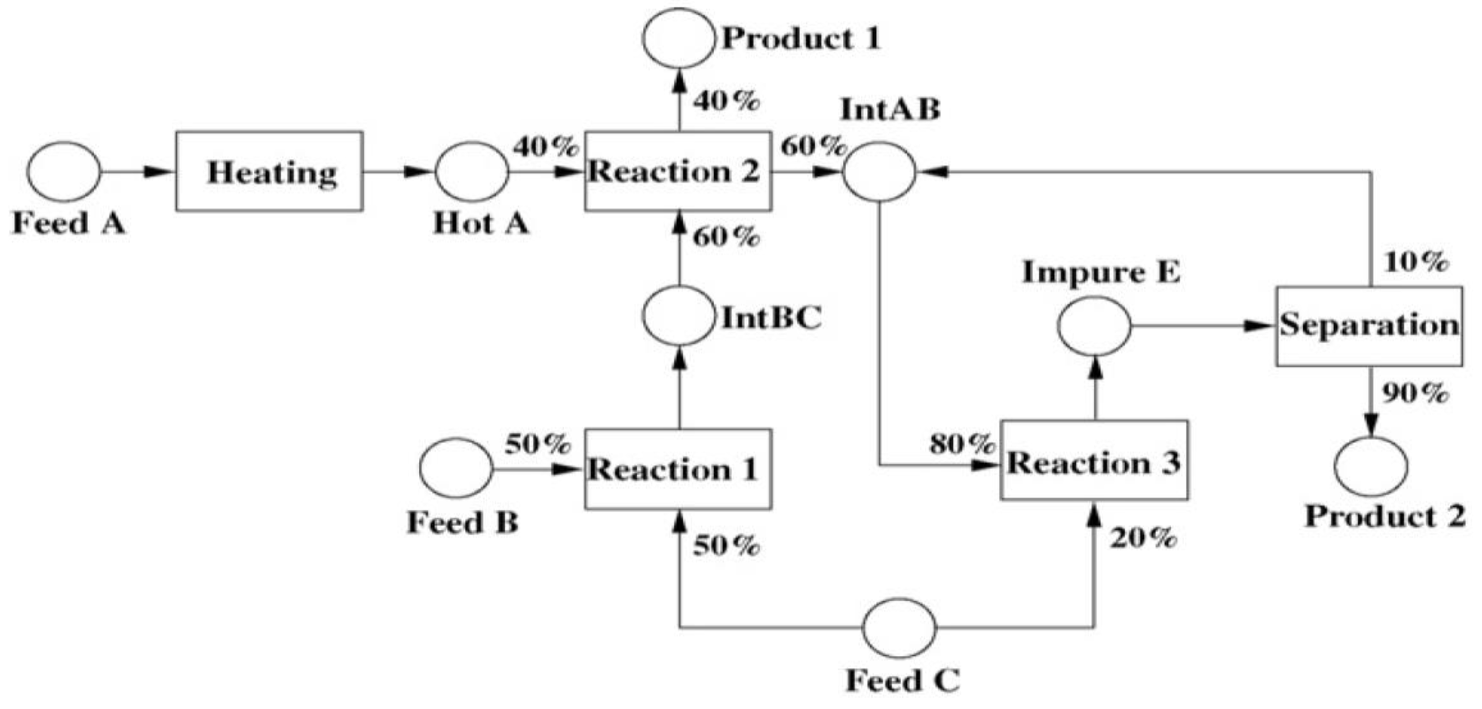


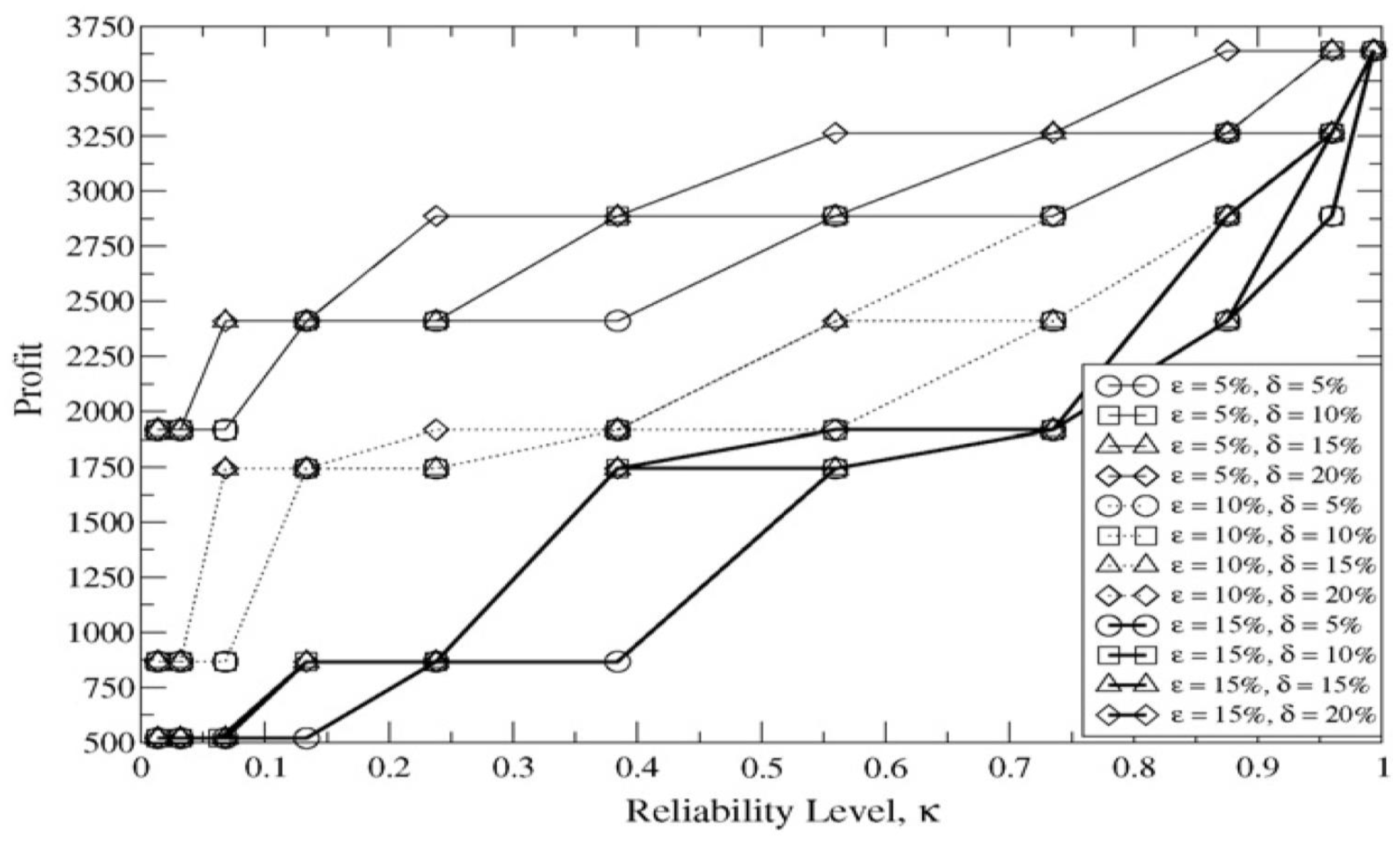


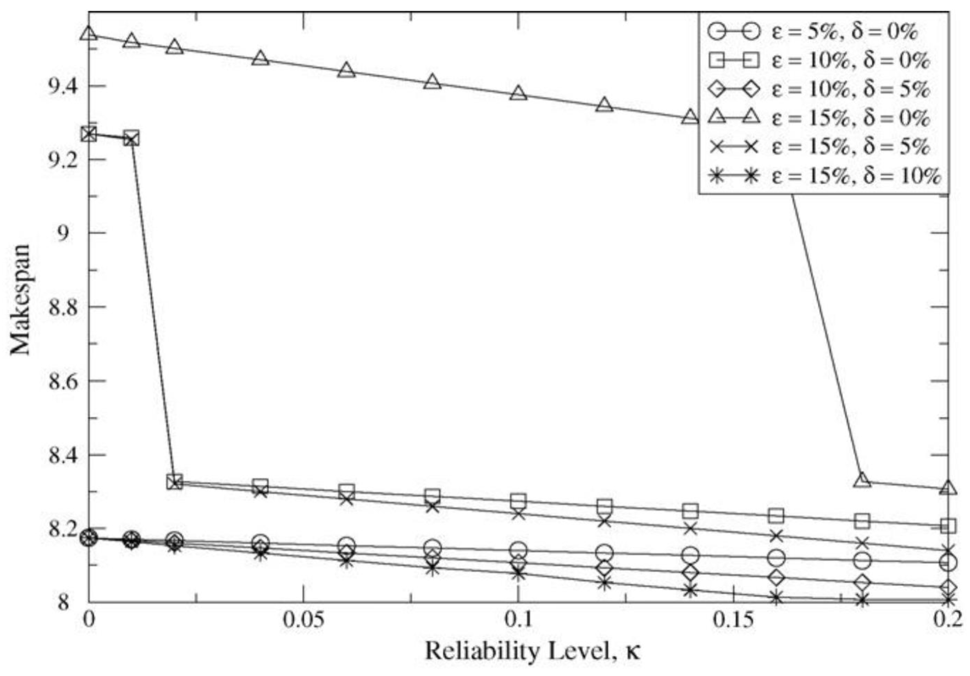


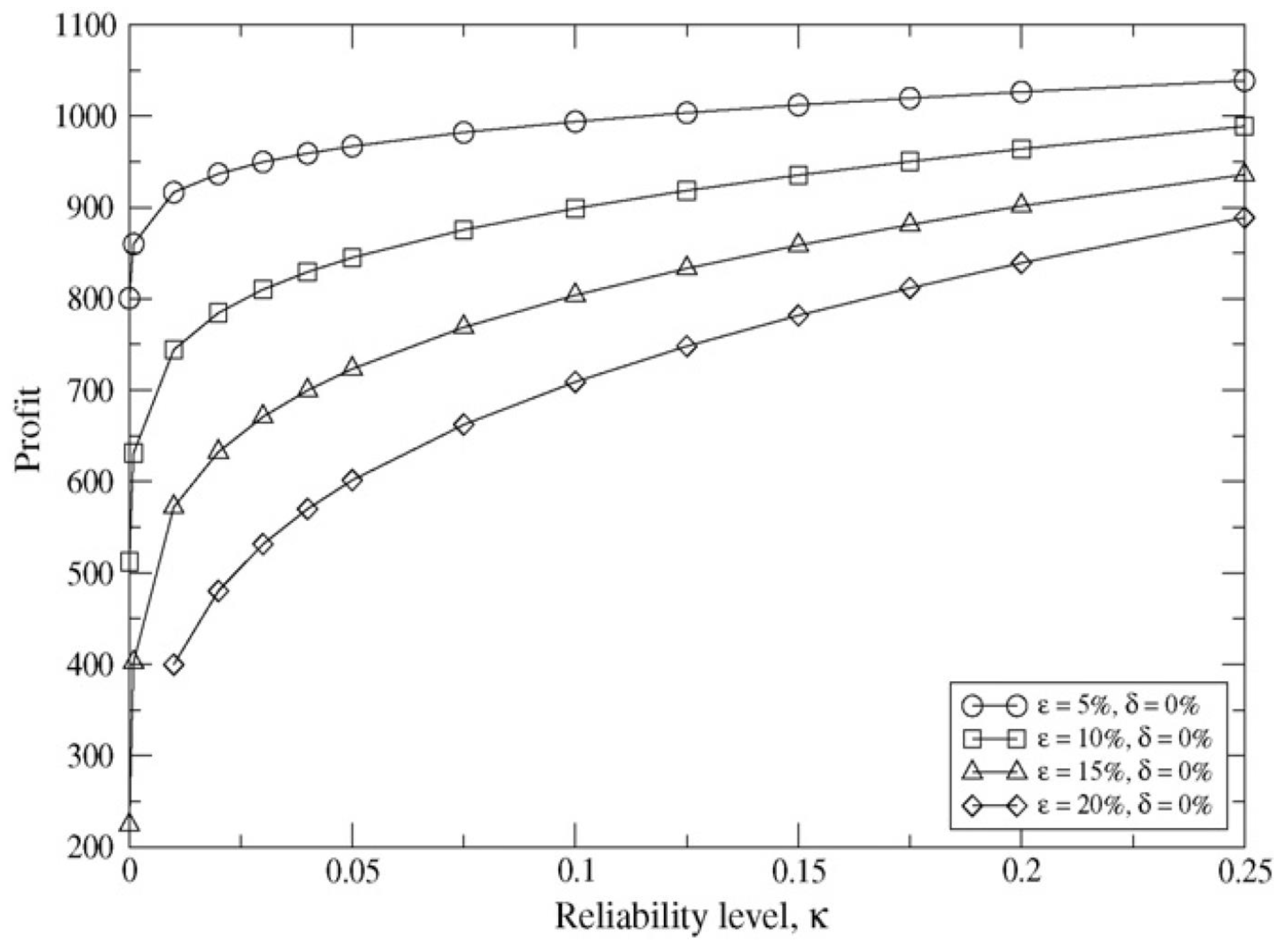
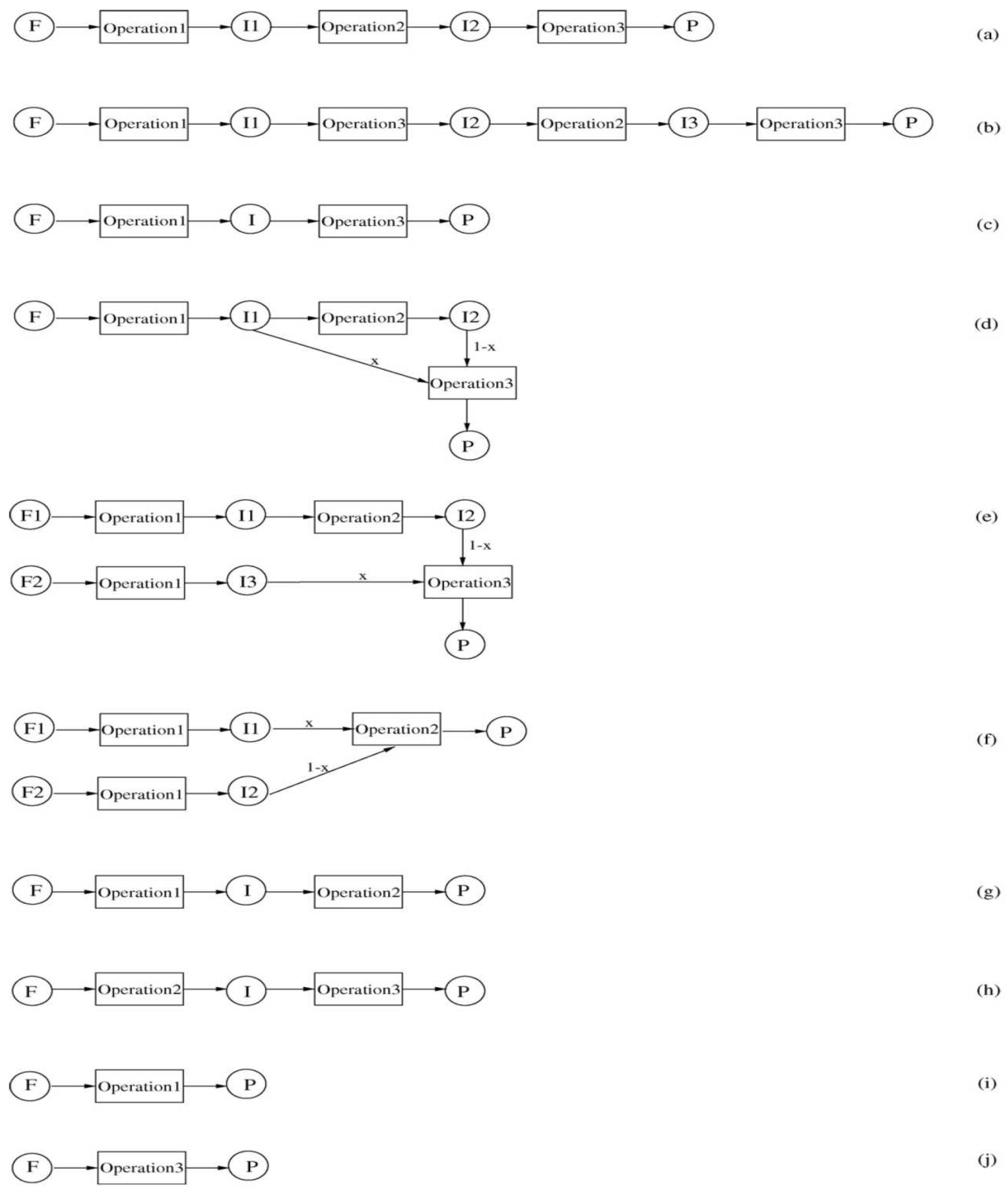
| Units | Adaptability | Process period | Capacity |
|---|---|---|---|
| Heater | Heating | 1.0 | 100 |
| Reactor 1 | R 1, 2, 3 | 2.0, 2.0, 1.0 | 50 |
| Reactor 2 | Reactions 1, 2, 3 | 2.0, 2.0, 1.0 | 80 |
| Separator | Separation | 2.0 | 200 |
| States | Initial Amount | Price | Storage |
| Feed A | Unbounded | 0 | Unbounded |
| Feed B | Unbounded | 0 | Unbounded |
| Feed C | Unbounded | 0 | Unbounded |
| Hot A | 0 | 0 | 100 |
| IntAB | 0 | 0 | 200 |
| IntBC | 0 | 0 | 150 |
| ImpureE | 0 | 0 | 200 |
| Product 1 | 0 | 10.0 | Unbounded |
| Product 2 | 0 | 10.0 | Unbounded |
| RS | NS | |
|---|---|---|
| Benefit CPU time (s) BIN variables CON variables Constraints |
2887.19 | 3638.75 |
| 11.33 | 0.46 | |
| 96 | 96 | |
| 442 | 442 | |
| 777 | 553 |
| RS | NS | |
|---|---|---|
| Make-span CPU time (s) BIN variables23 CON variables24 Constraints |
8.174 | 8.007 |
| 0.02 | 0.02 | |
| 60 | 60 | |
| 280 | 280 | |
| 409 | 375 |
| RS | NS | |
|---|---|---|
| Benefit CPU time (s) BIN variables CON variables Constraints |
966.97 | 1088.75 |
| 0.05 | 0.02 | |
| 60 | 60 | |
| 280 | 280 | |
| 334 | 334 |
| Units | ||||||||||
|---|---|---|---|---|---|---|---|---|---|---|
| Mission | 1 | 2 | 3 | 4 | 5 | 6 | 7 | 8 | 9 | 10 |
| 1 | 0 | 0 | 0 | 9.5 | -- | -- | -- | -- | -- | -- |
| 2 | -- | -- | -- | -- | 0 | 0 | 0.95 | -- | -- | -- |
| 3 | -- | -- | -- | -- | -- | -- | -- | 12 | 12.8 | 12.5 |
| 4 | 0 | 10 | 10 | 10 | -- | -- | -- | -- | -- | -- |
| 5 | -- | -- | -- | -- | 0.575 | 0.575 | 0.725 | -- | -- | -- |
| 6 | -- | -- | -- | -- | -- | -- | -- | 12 | 12.8 | 12.5 |
| 7 | 6.09 | 6.09 | 6.09 | 11.1 | -- | -- | -- | -- | -- | -- |
| 8 | -- | -- | -- | -- | 0.6 | 0.6 | 0.8 | -- | -- | -- |
| 9 | -- | -- | -- | -- | -- | -- | -- | 12.5 | 13.8 | 12.9 |
| 10 | 6.09 | 6.09 | 6.09 | 11.1 | -- | -- | -- | -- | -- | -- |
| 11 | -- | -- | -- | -- | 0.6 | 0.6 | 0.8 | -- | -- | -- |
| 12 | -- | -- | -- | -- | -- | -- | -- | 12.5 | 13.8 | 12.9 |
| 13 | 6.09 | 6.09 | 6.09 | 11.1 | 0.6 | 0.6 | 0.8 | -- | -- | -- |
| 14 | -- | -- | -- | -- | -- | -- | -- | -- | -- | -- |
| 15 | -- | -- | -- | -- | -- | -- | -- | 12.5 | 13.8 | 12.9 |
| 16 | -- | -- | -- | -- | 0.6 | 0.6 | 0.8 | -- | -- | -- |
| 17 | -- | -- | -- | -- | -- | -- | -- | 12.5 | 13.8 | 12.9 |
| 18 | 0 | 8.5 | 8.5 | 0 | -- | -- | -- | -- | -- | -- |
| 19 | -- | -- | -- | -- | -- | -- | -- | 0 | 15 | 16 |
| 20 | 0 | 0 | 8.38 | 9.5 | -- | -- | -- | -- | -- | -- |
| Mission | Unit | NVs | Uncertainty | Rang | Mean | SD. |
|---|---|---|---|---|---|---|
| 1 | 4 | 9.5 | N | -- | 9.912 | 0.523 |
| 7,10,13 | 1-3 | 6.09 | N | -- | 6.153 | 0.152 |
| 7,10,13 | 4 | 11.1 | B | 10.1-11.3 | -- | -- |
| 20 | 3 | 8.38 | B | 8.00-10.42 | -- | -- |
| 2 | 7 | 0.95 | N | -- | 0.9611 | 0.112 |
| 8,11,14,16 | 5-6 | 0.60 | B | 0.344-0.853 | -- | -- |
| 3,6 | 9 | 12.8 | B | 10.5-19.3 | -- | -- |
| 9,12,15,17 | 9 | 13.8 | B | 12.0-16.3 | -- | -- |
| 9,12,15,17 | 10 | 12.9 | N | -- | 12.100 | 0.760 |
| RS | NS | |
|---|---|---|
| Obj BIN variables CON variables Constraints CPU time (s) Nodes |
105.76 | 121.37 |
| 930 | 930 | |
| 6161 | 6005 | |
| 22931 | 18907 | |
| 5910 | 3880 | |
| 35640 | 15230 |
Disclaimer/Publisher’s Note: The statements, opinions and data contained in all publications are solely those of the individual author(s) and contributor(s) and not of MDPI and/or the editor(s). MDPI and/or the editor(s) disclaim responsibility for any injury to people or property resulting from any ideas, methods, instructions or products referred to in the content. |
© 2023 by the authors. Licensee MDPI, Basel, Switzerland. This article is an open access article distributed under the terms and conditions of the Creative Commons Attribution (CC BY) license (http://creativecommons.org/licenses/by/4.0/).


