Learning Data-Driven Stable Corrections of Dynamical Systems. Application to the Simulation of the Top-Oil Temperature Evolution of a Power Transformer

Preprint

Article

Learning Data-Driven Stable Corrections of Dynamical Systems. Application to the Simulation of the Top-Oil Temperature Evolution of a Power Transformer

Altmetrics

Downloads

Views

Comments

A peer-reviewed article of this preprint also exists.

Chady Ghnatios,

Xavier Kestelyn,Guillaume Denis,

Victor Champaney,

Francisco Chinesta^*

Chady Ghnatios,

Xavier Kestelyn,Guillaume Denis,

Victor Champaney,

Francisco Chinesta^*

This version is not peer-reviewed

Submitted:

26 June 2023

Posted:

27 June 2023

You are already at the latest version

Alerts

Abstract

Many engineering systems are described by using differential models whose solutions, generally obtained after discretization, can exhibit a noticeable deviation with respect to the response of the physical systems that those models are expected to represent. In those circumstances one possibility consists of enriching the model in order to reproduce the physical system behavior. The present paper considers a dynamical system, and proposes enriching the model solution by learning the dynamical model of the gap between the system response and the model-based prediction, while ensuring that the time integration of the learnt model remains stable. The proposed methodology is applied on the simulation of the top-oil temperature evolution of a power transformer, whose data is provided by RTE, the French Electricity Transmission System Operator.

Keywords:

Subject: Engineering - Electrical and Electronic Engineering

1. Introduction

The two most usual approaches involved in simulation based engineering –SBE–, the one mainly based on physics, and the more recent one, the one based on the use of data manipulated by advanced machine learning techniques, both present their inherent limitations.

In general, the physics-based modeling framework produces responses that approximate quite well the real ones, as soon as an accurate enough model exists. The main difficulties when considering such a physics-based approach are: (i) the fidelity of the model itself, assumed calibrated; (ii) the impact that variability and uncertainty induces; and (iii) the computing time required for solving the complex and intricate mathematical models.

On the other hand, the data-driven framework is not fully satisfactory, because even if the data (assumed noise-free) represent well the reality, its extrapolation or interpolation in space and time from the collected data (in particular locations and times instants) entail usually a noticeable accuracy loss.

Of course, by increasing the number of collected data, one could expect approximating the real solution with more fidelity, however, data is not always simple to collect, not always possible to access, and in all cases collecting data is expensive (cost of sensors, cost of communication and analysis, ...). Equipping a very large industrial or civil infrastructure with millions of sensors to cover all its spatial dimension seems simply unreasonable.

Moreover, even when the solution is properly approximated, two difficulties persist: (i) the solution explainability, compulsory to certify solutions and decisions; and (ii) the domain of validity when extrapolating far from the domain where data was collected.

In view of the limitations of both existing procedures, a gateway consists of allying both to conciliate agility and fidelity. The hybrid paradigm seems a valuable and appealing option. It considers the reality expressible from the addition of two contributions: the existing knowledge (the state-of-the-art physics-based model or any other kind of knowledge-based model) and the part of the reality that the model ignores, the so-called ignorance (also called deviation, gap, discrepancy, or simply, ignorance).

1.1. The three main SBE methodologies revisited

To introduce and discuss different simulation based engineering frameworks, we consider a certain field

u (x)

describing the evolution of the variable u along the space defined by the coordinates

x \in Ω \subset R^{D}

We assume that it exists a certain knowledge on the addressed physics, described by the model

M

, that in general consists of a system of algebraic equations or a system of differential equations complemented with the appropriate boundary and initial conditions ensuring the problem solvability. The solution provided by the just referred model, that as indicated, represents the existing knowledge on the problem at hand, is represented by

u^{M} (x)

Due to the partial knowledge on the addressed physical phenomenon, the calculated solution

u^{M} (x)

is expected to differ from the reference one

u (x)

, which is intended to be represented with maximum fidelity.

Thus, we define the residual

R^{M} (x)

according to

R^{M} (x) = u (x) - u^{M} (x),

(1)

where the error can be computed from its norm,

E^{M} = ∥ R^{M} (x) ∥

For reducing that error different possibilities exist:

Physics-based model improvement. This approach consists of refining the modelling, by enriching the model itself, $M \to \hat{M}$ , such that its solution $u^{\hat{M}}$ exhibits a smaller error, i.e. $E^{\hat{M}} \leq E^{M}$ .
Fully data-driven description. The data-driven route consists of making a large sampling of the space $Ω$ , $x_{1}, . . ., x_{P}$ , with $P$ large enough, and with the points location $x_{i}$ , $i = 1, . . ., P$ , maximizing the domain $Ω$ coverage. These points are grouped into the set $S$ .

The coverage is defined by the convex hull $ω (S)$ of the set $S = {x_{1}, . . ., x_{P}}$ , ensuring interpolation for $x \in ω (S)$ , limiting the risky extrapolation to the region of $Ω$ outside the convex hull $ω (S)$ .

Factorial samplings try to maximize the coverage, however factorial samplings, or the ones based on the use of Gauss-Lobatto quadratures, related to approximations making use of orthogonal polynomials [3], fail when the dimensionality of the space $D$ increases.

When $D ≫ 1$ , sparse sampling is preferred, LHP (Latin hyper cube) for instance. Samplings based on gaussian processes –GP– aim at distributing the points in locations where the uncertainty is maximum (with respect to the predictions inferred from the previously collected data).

Finally, the so-called active learning techniques drive the sampling aiming at maximizing the representation of a certain goal oriented quantity of interest [32].

In what follows, we assume a generic sampling to access to the reference solution $u (x_{i})$ , $i = 1, . . ., P$ , assuming a perfect measurability.

Now, to infer the solution at $x \in ω (S)$ , it suffices constructing an interpolation or approximation, more generally, an adequate regression $u^{S} (x)$ :

$u^{S} (x) \equiv u (x; u_{1}, . . ., u_{P}),$

(2)

with $u_{1} \equiv u (x_{1}), . . ., u_{P} \equiv u (x_{P})$ .

Different possibilities exist, among them: regularized polynomial regressions Please rearrange all the references to appear in numerical order. [29], neural networks –NN– [16,31], support vector regression –SVR– [9], decision trees and their random forest counterparts [4,23], ... to name few.

The trickiest issue concerns the error evaluation, that is quantified from a part of the data kept outside the training-set, the so-called test-set, used to quantify the performances of the trained regression.

The main drawbacks of such a general procedure, particularly exacerbated in the multi-dimensional case ( $D ≫ 1$ ), are the following:

–

Ability to explain the regression $u^{S} (x)$ .

–

The size of the data-set ( $P$ ), scaling with the problem dimensionality $D$ .

–

The optimal sampling to cover $Ω$ while guaranteeing the accuracy of $u^{S} (x)$ , or the one of the goal oriented quantities of interest.
Hybrid approach. It proceeds by embracing the physics-based and data-driven approaches, that as described in the next section, will improve the physics-based accuracy (while profiting of the physics-based explanatory capabilities) from the use of a data-driven enrichment, that at its turn, and under certain conditions, needs less amount of data than the fully data-driven approach just discussed [6].

2. Illustrating the hybrid approach

2.1. A simple linear regression reasoning

In the hybrid approach we consider first the contribution of a model expected representing reasonably the physics at hand, and noted by

u (x)

, and that was noted previously as

u^{M} (x)

, with

x \in Ω \subset R^{D}

As discussed before, it entails a residual

R^{M} (x)

and the associated error,

E^{M}

Imagine for a while the simplest (and cheapest) regression of that residual, a linear regression involving

P

data, associated with the locations

x_{i} \in Ω, i = 1, . . ., P

Thus, the linear regression involving a linear approximation of the residual, noted by

Δ u^{L} (x)

reads:

Δ u^{L} (x; a_{0}^{Δ}, . . ., a_{D}^{Δ}) = a_{0}^{Δ} + a_{1}^{Δ} x_{1} + . . . + a_{D}^{Δ} x_{D},

(3)

that involve the unknown coefficients

a_{0}^{Δ}, a_{1}^{Δ}, . . ., a_{D}^{Δ}

By using the L2-norm, the linear regression results from the least-square minimization problem:

{a_{0}^{Δ}, . . ., a_{D}^{Δ}} = {argmin}_{a_{0}^{*}, . . ., a_{D}^{*}} \{\sum_{i = 1}^{P} {(Δ u^{L} (x_{i}; a_{0}^{*}, . . ., a_{D}^{*}) - R^{M} (x_{i}))}^{2}\},

(4)

that defines an interpolation in the case

P = D + 1

and an approximation when

P \geq D + 1

If we assume for a while that

u (x)

is fully available, and then

R^{M} (x)

too, the previous expression can be rewritten in a continuous form

{a_{0}^{Δ}, . . ., a_{D}^{Δ}} = {argmin}_{a_{0}^{*}, . . ., a_{D}^{*}} {∥ Δ u^{L} (x; a_{0}^{*}, . . ., a_{D}^{*}) - R^{M} (x) ∥}_{2} .

(5)

The linear regression of the reference solution

u (x)

, noted by

u^{L} (x; a_{0}^{u}, . . ., a_{D}^{u})

, reads at its turn

u^{L} (x; a_{0}^{u}, . . ., a_{D}^{u}) = a_{0}^{u} + a_{1}^{u} x_{1} + . . . + a_{D}^{u} x_{D},

(6)

where the coefficients

a_{0}^{u}, . . ., u_{D}^{u}

results again from the least-square minimization problem

{a_{0}^{u}, . . ., a_{D}^{u}} = {argmin}_{a_{0}^{*}, . . ., a_{D}^{*}} \{\sum_{i = 1}^{P} {(u^{L} (x_{i}; a_{0}^{*}, . . ., a_{D}^{*}) - u (x_{i}))}^{2}\},

(7)

whose continuous expression reads

{a_{0}^{u}, . . ., a_{D}^{u}} = {argmin}_{a_{0}^{*}, . . ., a_{D}^{*}} {∥ u^{L} (x; a_{0}^{*}, . . ., a_{D}^{*}) - u (x) ∥}_{2} .

(8)

Eq. (5) implies

∥ Δ u^{L} (x; a_{0}^{Δ}, . . ., a_{D}^{Δ}) - R^{M} (x) ∥_{2} \leq {∥ R^{M} (x) ∥}_{2} .

(9)

Thus, as soon as the error related to the residual becomes smaller than the one related to the linear approximation of the reference solution, i.e. if

E^{M} = ∥ R^{M} {(x) ∥}_{2} \leq {∥ u^{L} (x, a_{0}^{u}, . . ., a_{D}^{u}) - u (x) ∥}_{2},

(10)

then

∥ Δ u^{L} (x; a_{0}^{Δ}, . . ., a_{D}^{Δ}) - R^{M} (x) ∥_{2} \leq ∥ R^{M} (x) ∥_{2} \leq {∥ u^{L} (x, a_{0}^{u}, . . ., a_{D}^{u}) - u (x) ∥}_{2},

(11)

that proves the higher accuracy of the hybrid approximation as soon as the solution provided by the model

M

represents a better approximation to the reference solution

u (x)

than a linear regression could attain.

2.2. General remarks

The analysis just addressed considers a simple linear regression involving a linear approximation, however it remains valid when considering regressions involving richer nonlinear approximations.

The first part of Eq. (11), i.e.

∥ Δ u^{L} (x; a_{0}^{Δ}, . . ., a_{D}^{Δ}) - R^{M} (x) ∥_{2} \leq {∥ R^{M} (x) ∥}_{2},

affirms that the simulated model solution is enriched in a L2-norm sense, and under the constraint of having enough amount of data to evaluate the considered norms. It is important to note, that even if the simulated model solution is enriched in the L2-norm sense, locally, the accuracy of the enriched solution could be degraded.

The second part pf Eq. (11), i.e.

∥ R^{M} {(x) ∥}_{2} \leq {∥ u^{L} (x, a_{0}^{u}, . . ., a_{D}^{u}) - u (x) ∥}_{2},

works under some conditions involving the data and the model, i.e. on

u (x)

and

u^{M} (x)

, to be checked, and again needs having an amount of data enabling the calculation of the L2-norms.

2.3. On the domain of application of the hybrid modeling approach

The hybrid approach applies in different settings. It can be viewed as a sort of transfer learning, where rich behaviors are approached from others close enough and well stablished.

This hybrid approach seem particularly appealing in different situations, as the ones reported below:

When the model captures most of the solution features, the correction must describe a discrepancy that exhibits smaller nonlinearities, as was the case treated in [27,28], where the same amount of data performed better within the hybrid than within the fully data-driven framework.
Sometimes, the physics-based model operates very accurately in a part of the domain, whereas strong nonlinearities localize in a small region that can, in that case, be captured by a data-driven learned model, as considered in [26] for addressing the inelastic behavior of spot-welds.
When considering the constitutive modeling of materials, the augmented rationale (or hybrid paradigm) expresses the real behavior from a first order behavior (calibrated from the available data) complemented by an enrichment (or correction) filling the gap between the collected data and the predictions obtained from the assumed model [15].
When addressing plates (or shells) which noticeable 3D behaviors (deviating from the usual shell theory) a valuable solution consists of using an enriched kinematics consisting of two contributions: the first order one (usual shell kinematics) enriched with a second order contribution [25], that can be learned from data.
The hybrid modeling can also transfer the existing knowledge slightly outside its domain of applicability with small amount of collected data, as performed in [24] for correcting state-of-the-art structural beam models.
Sometimes the discrepancy concerns an imperfect alignment of the solution between the prediction and the measures. That discrepancy seems very high when evaluating it at each location, however, a small transport allows aligning both solutions. Optimal transport is very suitable in these situations, where the hybrid model consists of the usual nominal model enriched from a parametric correction formulated in an optimal transport setting as described in [34,35].
In [20] a correction of a Mises yield function was performed from the deviation between the results predicted by using it, and the measures obtained at the structure level.
Finally, when addressing processing and performances, the hybrid formulation, of different granularities, can exhibit advantages (amount of data, ability to explain, knowledge transfer, ...), at the heart of the digital twin developments [1,5,6,13,14,21,36].

3. Methods

In what follows, a system characterized by the state x that evolves in time, i.e.

x (t)

, is considered, and the stability of its numerical integration discussed [11]. When the state is multi-valued it will be noted by

x

3.1. On the integration stability

We consider for a while a simple linear dynamical system expressed by

\frac{d x}{d t} = a x, a \in R .

(12)

The integration reads

\frac{d x}{x} = a d t \to \ln (x) = C + a t \to x (t) = \hat{C} e^{a t},

(13)

with

\hat{C} = e^{C}

and

\hat{C} = x (t = 0)

It can be noticed that the existence of a bounded solution requires that

a \leq 0

, because if

a > 0

x (t \to \infty) = \infty

. Thus, the stability condition writes

a \leq 0

Now, we consider the discrete case, in which the first order derivative is discretized by a first order finite difference

\frac{d x}{d t} = \frac{x_{n} - x_{n - 1}}{Δ t},

(14)

where

x_{n} = x (t = t_{n})

, with

t_{n} = n Δ t

In that case, the discrete time evolution reads

x_{n} = a x_{n - 1} Δ t + x_{n - 1} = (a Δ t + 1) x_{n - 1} = b x_{n - 1},

(15)

with

b = (a Δ t + 1)

Now because

x_{n - 1} = b x_{n - 2}

, and so on, it finally results

x_{n} = b^{n} x_{0},

(16)

from which it can be concluded that bounded solutions are subjected to the constraint

b \leq 1

Similar results can be obtained in the case of multi-valued states. In what follows we consider the differential system

\frac{d x}{d t} = A x .

(17)

For the sake of simplicity we assume that matrix

P

diagonalizes

A

, with

P^{T} P = I

(

I

is the unit matrix). Thus, if we define

x = P y

, it results

P \frac{d y}{d t} = A P y,

(18)

that premultiplying by

P^{T}

results

P^{T} P \frac{d y}{d t} = P^{T} A P y,

(19)

that taking into account that

P^{T} P = I

, can be rewritten as

\frac{d y}{d t} = D y,

(20)

with

D

diagonal.

The fact of being

D

diagonal, allows decoupling the solution of Eq. (20). Thus, we have

\frac{d y_{i}}{d t} = D_{i} y_{i}, \forall i,

(21)

with

y_{i}

the i-component of

y

and

D_{i}

the

(i, i)

-diagonal component of

D

Thus, using the previous results, the stability condition reads

\max_{i} D_{i} \leq 0 .

(22)

By discretizing Eq. (20), it results

y_{n} = (Δ t D + I) y_{n - 1},

(23)

or notting

\hat{D} = Δ t D + I

y_{n} = \hat{D} y_{n - 1},

(24)

that using the recurrence results in

y_{n} = {\hat{D}}^{n} y_{0} .

(25)

Thus, stability requires the spectral radius

ρ

\hat{D}

being lower than the unity, i.e.

ρ (\hat{D}) \leq 1

These conditions should be satisfied by the dynamical learned models, as discussed later.

3.2. Learning integrators

When the dynamical system is know, different numerical integration schemes (explicit, implicit or semi-implicit) can be applied, with different convergence orders, for instance the Euler, or the more accurate Runge-Kutta, among many other choices. Thus, the discretization time-step

Δ t

must be chosen to ensure stability, and to guarantee convergence, that is, a numerical solution close enough to the reference solution of the problem.

In what follows, we revisit, and discuss, different machine learning techniques that enable learning dynamical systems and applying them for the integration of dynamical systems, as recurrent NN –rNN– and long short time memory –LSTM– techniques perform [10,37].

In this section

h

refers to the hidden state, whereas

l

and

o

refer, respectively, to the inputs (loading) and observable outputs.

3.2.1. Recurrent Neural Network

W^{•}

represents dense matrices associated to variables •,

σ (\cdot)

the activation function,

h_{n}

the internal state at the n-time step,

t_{n}

, and

l_{n}

and

o_{n}

the associated input and output at the present time

t_{n}

, then the rNN proceeds from:

\{\begin{matrix} h_{n} = σ^{h} (W^{h} h_{n - 1} + W^{l} l_{n}) \\ o_{n} = σ^{y} (W^{o} h_{n}), \end{matrix},

(26)

whose architecture is depicted in Figure 1.

To perform the time evolution it suffices to use the rNN and re-inject the rNN output

h_{n}

, as the input at the next time step.

A temporal sequence of inputs and outputs, assumed available, allows calculating the different weights composing the different

W

matrices.

To highligth the connexion between the rNN and usual dynamical system integrators, we consider for a while the finite element semi-discretized form of a linear parabolic differential equation

M \frac{d h}{d t} = K h + l,

(27)

where

M

and

K

are two matrices that results from the spatial discretization. Here,

h

refers to the state and

l

to the system loading.

Then, the explicit discretization of Eq. (27) reads

M h_{n} = Δ t K h_{n - 1} + Δ t l_{n} + M h_{n - 1} = (Δ t K + M) h_{n - 1} + Δ t l_{n},

(28)

from which the state updating results

h_{n} = M^{- 1} (Δ t K + M) h_{n - 1} + Δ t M^{- 1} l_{n},

(29)

that can be rewritten as

h_{n} = W^{h} h_{n - 1} + W^{l} l_{n},

(30)

that correspond to the particularization of Eq. (26) to the linear case. Thus, the intimate connexion between rNN and usual discretization techniques becomes explicit. The last operates on a known model whereas the former learns the model itself (the different

W^{•}

matrices).

Remark 1. In the just discussed linear model, when the whole state is observed, i.e.

o_{n} = h_{n}

W^{o} = I

3.2.2. On the model memory

When considering a first order dynamical system, as just discussed, the solution at the present time can be computed from the only knowledge of the previous solution (at the previous time step) and the present loading (also known as action or input). Thus, one could imagine that for learning first order dynamical systems a short memory, as for instance the one of the just described rNN, suffices.

However, sometimes, larger memory are needed even when addressing first order models as described in this section.

For the sake of simplicity we consider the system state given by

h (t) = {(h_{1} (t), h_{2} (t))}^{T}

, whose evolution is governed by a simple linear first order dynamical system

\{\begin{matrix} {\dot{h}}_{1} (t) = K_{11} h_{1} (t) + K_{12} h_{2} (t) + l_{1} (t) \\ {\dot{h}}_{2} (t) = K_{21} h_{1} (t) + K_{22} h_{2} (t) + l_{2} (t) \end{matrix},

(31)

where, without loss of generality, it is assumed

K_{22} = 0

and

l_{2} (t) = 0

, i.e.

\{\begin{matrix} {\dot{h}}_{1} (t) = K_{11} h_{1} (t) + K_{12} h_{2} (t) + l_{1} (t) \\ {\dot{h}}_{2} (t) = K_{21} h_{1} (t) \end{matrix} .

(32)

In what follows, it is assumed that

h_{1} (t)

and

x_{1} (t)

are accessible, but that nothing, even the existence of

l_{2} (t)

, is known. In that circumstances the key question is: can we learn a model relating

l_{1} (t)

and

h_{1} (t)

, both accessible and measurable, knowing that the state

h_{1} (t)

depends on another one,

h_{2} (t)

, that evolves in time and remains inaccessible, and consequently unknown.

To facilitate the model manipulation, the Fourier transform applies, here noted by the symbol

\cdot^{*}

, acting on the different time-dependent variables. Thus, Eq. (32) writes

\{\begin{matrix} i ω h_{1}^{*} = K_{11} h_{1}^{*} + K_{12} h_{2}^{*} + l_{1}^{*} \\ i ω h_{2}^{*} = K_{21} h_{1}^{*} \end{matrix} .

(33)

From the second equation in (33) we obtain

h_{2}^{*} = K_{21} \frac{h_{1}^{*}}{i ω}

(34)

that inserted in the first equation in (33) leads to

i ω h_{1}^{*} = K_{11} h_{1}^{*} + K_{12} K_{21} \frac{h_{1}^{*}}{i ω} + l_{1}^{*},

(35)

that coming back to the time domain results

\frac{d h_{1} (t)}{d t} = K_{11} h_{1} (t) + K_{12} K_{21} \int_{0}^{t} h_{1} (τ) d τ + l_{1} (t),

(36)

that proves that ignoring components of the state manifests in the measurable state history, here symbolized by the integral. In a certain way, this result can be interpreted as a consequence of the Taken delay embedding theorem.

Thus, memory is not only a consequence of the order of the subjacent dynamics, the memory in the learning procedure also depends on the ignored states. Thus, sometimes, when addressing poorly described physical systems or partially accessible, larger memory than the one that recurrent NN offers, seems compulsory.

3.2.3. Learners with larger memory

LSTM (Long Short Time Memory) [19] becomes an appealing technique for learning time-dependent problems while ensuring larger memory. LSTM combines a short and a long time memory units, with an evanescent memory for the long-time path, and a combination of long and short leads to the short memory response..

A particular architecture is depicted in Figure 2, that is considered for including not only memory, but also the previous inputs as well as forgetting the initial conditions of the long

c_{0}

and short

h_{0}

memory channels, to facilitate its use as a generic time integrator.

Recurrent NN (rNN) and LSTM learn the state evolution, and special care must be paid to ensure time integration stability.

Sometimes it seems preferably learning the forcing term of the dynamical system, as Residual Nets or Neural Differential Equations techniques perform. Next section revisits Residual Nets and discuss stability issues.

3.2.4. Residual Nets

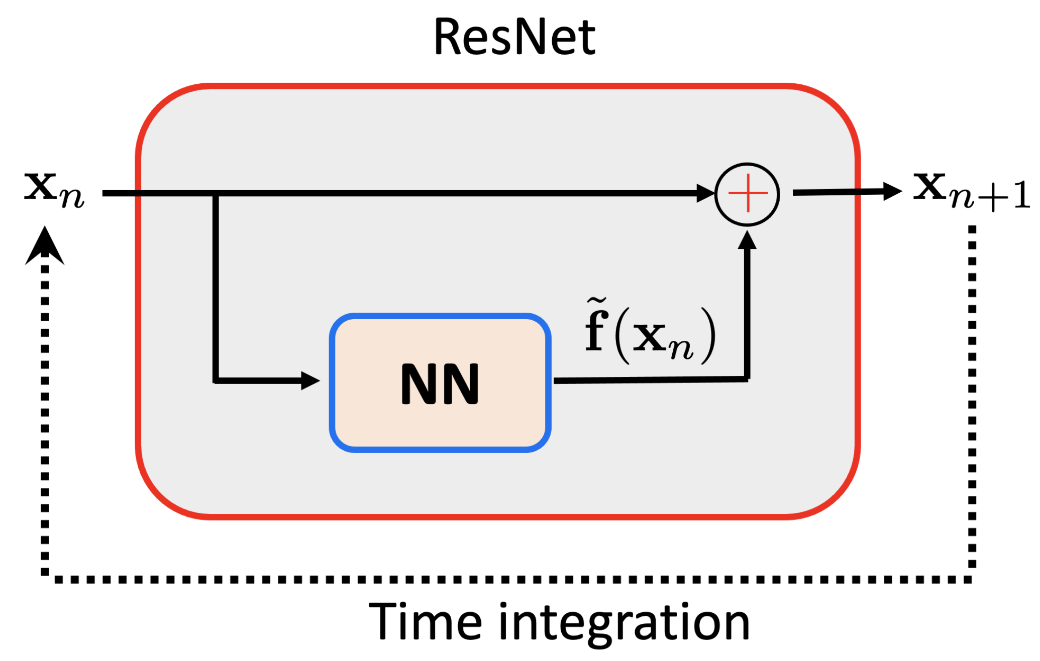
Residual Neural Networks (ResNet) [2,17,18] aim at emulating the backward integration of a dynamical system. When we consider the dynamical system

\frac{d x}{d t} = f (x), x (t = 0) = x_{0},

(37)

the ResNet looks for the function

f (x)

that allows reproducing the state time evolution

x (t)

, from its discrete knowledge, that is, from

x_{n} = x (t_{n})

, with

t_{n} = n Δ t

By considering the simplest time stepping, the time derivative can be approximated by

d x / d t = (x_{n + 1} - x_{n}) / Δ t

, and then, one can use the following updating

x_{n + 1} = x_{n} + Δ t f (x_{n}),

(38)

and learn the forcing term

f (x)

that induced the state evolution by using an appropriate regression.

For that purpose ResNet creates a NN trained from

x_{n}

and

x_{n + 1} - x_{n}

n = 1, . . .

. Then, as soon as the NN is trained, the output

x_{n + 1}

is calculated by applying on

x_{n}

the NN just constructed adding the identity operator applied on the input.

Now, the dynamical system integration consists in applying in a recursive way the ResNet, with the output at time n becoming the input of the next time-step. The ResNet architecture and the integration procedure are illustrated in Figure 3.

4. Simple procedures for stabilizing ResNets-based integration

In what follows, the stabilization of the time integration performed with ResNet is discussed. First, a simple stabilization is accomplished by linearizing the dynamical system, while using of the results just discussed.

Then, inspired by that accomplishment, a more general stabilization, able to operate in nonlinear settings, is proposed.

Finally, the performances of both strategies are compared.

4.1. Learning stable linear dynamical systems

In what follows we consider a parametrized dynamical system,

\frac{d x}{d t} = f (x; z),

(39)

where the state at time

t_{n}

x_{n}

, depends on the previous state

x_{n - 1}

and the loading

f (\cdot)

driving the state change. The last is assumed depending not only on the state, but also on a series of parameters (input features) here grouped in vector

z

. Thus, the learning procedure aims at computing the regression

f (x; z)

However, for obtaining a stable integrator, certain constraints must be fulfilled. As these constraints have an easy form in the linear case, as previously discussed, here we proceed to linearize the forcing term as follows

f (x; z) \approx g (z) x + h (z) .

(40)

Now, the stability is ensured as soon as

g (z) \leq 0

, constraint that can be easily enforced by employing a penalty term in the loss function of the NN associated with

g (z)

The linearized ResNet resembles to the DMD (dynamic mode decomposition) [30], with probably an easier introduction of the parametric dimension.

4.2. Learning stable nonlinear dynamical systems

Inspired from the just discussed rationale, a possible route for enforcing stability without detriment of the nonlinear behavior consists of writing

f (x; z) \approx g (z, x) x + h (z) .

(41)

while enforcing in the construction of regression

g (x; z)

the negativity constraint, that is,

g (x; z) \leq 0

4.3. Numerical examples and discussion

To prove the expected performances we consider two cases, one linear, where both methodologies just described should work, and a nonlinear one, where the former is expected failing, whereas the later (the nonlinear counterpart) is expected performing correctly.

This section only addresses the stability concerns, without giving details on the neural architectures employed for learning functions

g (z)

g (x; z)

and

h (z)

, that will be described in detail in Section 5. Moreover, when the learnt functions are employed for integrating the dynamical system incrementally, by using a standard first order explicit time-marching, the computed solution will be noted with hat symbol,

\hat{\cdot}

4.3.1. Linear dynamical system

We consider data generated from the integration of the dynamical system

\frac{d x}{d t} = 1 - x,

(42)

integrated from the initial condition

x (t = 0)

= 0.

The long-time solution

x = 1

is stable, because if

x < 1

the solution increases, whereas if

x > 1

, it decreases.

The solution reads

x (t) = 1 - e^{- t},

(43)

that is used for generating the synthetic data that will be used then, for learning the dynamical system by using the two procedures previously described.

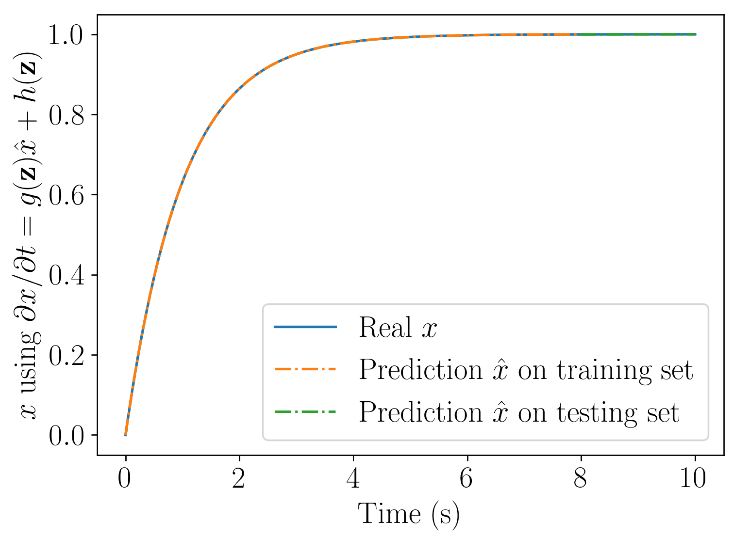
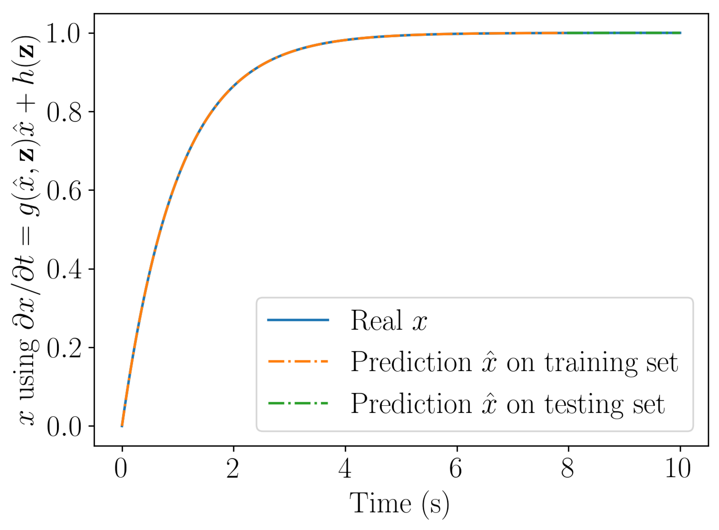
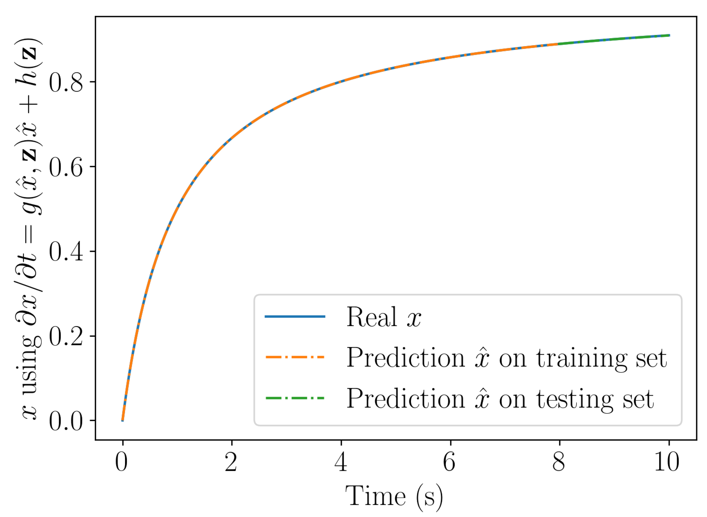
Figure compares the solution obtained by integrating numerically the models learnt by employing both, the linear and nor linear learning procedures. The problem being linear both procedures are expected performing identically, as Figure proves.

4.3.2. Nonlinear dynamical system

Now, a nonlinear dynamical system is considered, expressed by

\frac{d x}{d t} = {(1 - x)}^{2},

(44)

integrated from the initial condition

x (t = 0)

= 0.

Using the same rationale than before, we can conclude on the stability of the associated long-time solution

x = 1

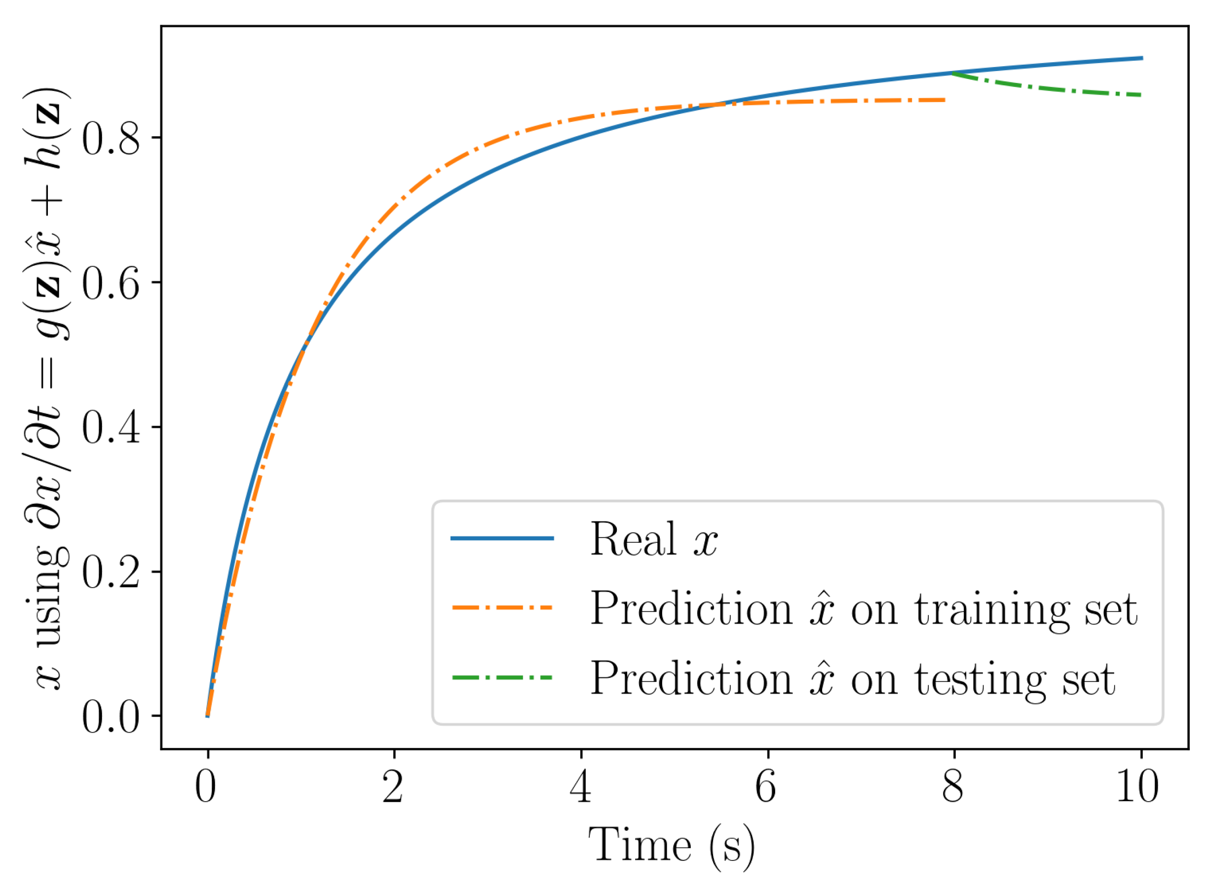
Figure 5 compares the solution obtained with the linear and nonlinear learning procedures. As expected, the nonlinear learning procedure ensures stability and represents accurately the nonlinear behavior, whereas the learnt linear model results stable but remains inaccurate.

4.4. Final remarks

Another potential neural architecture with improved robustness with respect to stability is the NeuralODE [7,8,12], that learns the model while considering many integration steps, instead of learning for one-step time increments as ResNet performs. Even is stability is significantly enhanced, the NeuralODE training efforts are higher than the ones required by the ResNet, mainly due to the fact that the back-propagation in the loss function minimization needs the solution of an adjoint problem, that, in some cases exhibits poor convergence.

5. Application to the evaluation of the top-oil temperature of an electric power transformer

This section addresses an applicative case of industrial relevance. Aging of transformers exhibits a correlation with the temperature of the oil all along their lives in service, and moreover, the oil temperature seems to be an appealing feature to anticipate faults, and consequently to be used in predictive maintenance.

Some simplified models exist to evaluate the oil temperature depending on the transformer delivered power and the ambient temperature. Standards propose different simplified models for that purpose, as the one considered later.

Because of the complexity of a transformer, large in size and embracing numerous physics and scales, an appealing modeling route consists of using a simplified model and then enrich it from the available collected data [22].

The just referred correction comes from the time-integration of a dynamical system, involving a parametric loading (delivered power and ambient temperature), learnt from the available data under the stability constraints.

To illustrate the construction of the enriched model for the top oil temperature prediction

Θ

, we consider as input the ambient temperature

T^{a m b}

, and the transformer load

K^{l o a d}

, which are both measured every hour. Thus, the model parameters read

z = {(T^{a m b}; K^{l o a d})}^{T}

The transformer oil temperature results from

Θ (t) = Θ^{T O} (t) + d (t),

(45)

where

d (t)

represents the deviation, and

Θ^{T O}

the temperature predicted by a state-of-the-art simplified model [33]:

\{\begin{matrix} P (K^{l o a d}, Θ^{W}, X^{t p}) = C_{t h} \frac{d Δ Θ^{T O}}{d t} + \frac{Δ Θ^{T O}}{R_{t h}} \\ Θ^{T O} = T^{a m b} + Δ Θ^{T O} \\ Θ^{W} = Θ^{T O} + Δ Θ^{O W} \end{matrix}

(46)

where

$X^{t p}$ : The position of the tap-changer;
$K^{l o a d}$ : the load factor, a ratio between the nominal load current and the actual current;
P: represents the iron, copper and supplementary losses. The power that heats the oil is composed of the losses that do not depend on the transformer load (iron losses, supposed constant) and the losses that depend on the transformer load (copper and supplementary losses) that depend on the average windings temperature and the load factor, according to: $P = P_{0} + P_{l o a d}$ , with $P_{l o a d} = K {^{l o a d}}^{2} P_{l o a d_{r}}$ and $P_{l o a d_{r}} = k P_{J o u l e_{r}} + \frac{P_{s u p p_{r}}}{k}$ (k being a correction factor related to the material resistivity);
$T^{a m b}$ : The ambient temperature;
$Θ^{T O}$ : The simulated top oil temperature
$Δ Θ^{T O}$ : The temperature difference between the simulated top oil temperature and the ambient temperature;
$R_{t h}$ and $C_{t h}$ : thermal resistance and thermal capacitance of the equivalent transformer thermal circuit;
$Θ^{W}$ : The average winding temperature;
$Δ Θ^{O W}$ : The difference between the average winding temperature and the simulated oil temperature $Θ^{T O}$ . It is supposed constant and found during the commissioning test (standards)

The physics-based model (46) is calibrated from the available experimental data, from which, parameters

C_{t h}

and

R_{t h}

are obtained. Two physics-based models are used, a linear one where

C_{t h}

and

R_{t h}

are assumed constant, and a nonlinear physics-based model where

C_{t h}

and

R_{t h}

are temperature dependent, that is, both coefficients depend on the top-oil temperature

Θ^{T O}

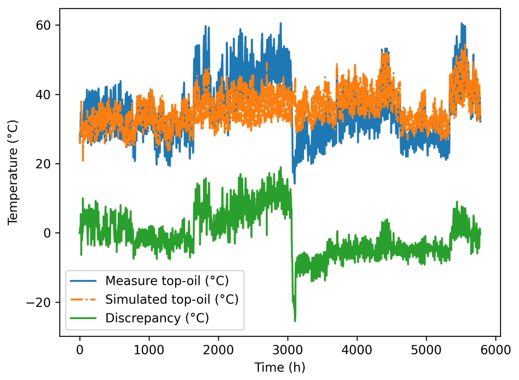
The available experimental data

Θ (t)

, the prediction from the calibrated physics-based non-linear model (46),

Θ^{T O} (t)

, and the deviation between both them,

d (t) = Θ (t) - Θ^{T O}

, are all depicted in Figure 6.

The model correction (the deviation model,

d (t)

) is obtained also using two different approaches: the linearized ResNet:

\frac{\partial d}{\partial t} = g (\tilde{z}) d + h (\tilde{z}),

(47)

and the nonlinear ResNet counterpart:

\frac{\partial d}{\partial t} = g (\tilde{z}, d) d + h (\tilde{z}),

(48)

where

\tilde{z}

represents the augmented features set, that contains the physical features

z

augmented with the model prediction

Θ^{T O}

Functions

g (\tilde{z})

and

h (\tilde{z})

are described by using two LSTM architectures (described in Table 1 and Table 2 respectively for the linearized ResNet) that consider the extended features involved in

\tilde{z}

at the present time, as well as at the previous 4 time-steps.

Thus, the linearized correction dynamical model reads

\{\begin{matrix} d_{n} = Δ t g (\tilde{z}) d_{n - 1} + Δ t h (\tilde{z}) + d_{n - 1} \\ \tilde{z} = (\begin{matrix} T_{n - 4}^{a m b} & K_{n - 4}^{l o a d} & Θ_{n - 4}^{T O} \\ T_{n - 3}^{a m b} & K_{n - 3}^{l o a d} & Θ_{n - 3}^{T O} \\ ⋮ \\ T_{n}^{a m b} & K_{n}^{l o a d} & Θ_{n}^{T O} \end{matrix}) \end{matrix} .

(49)

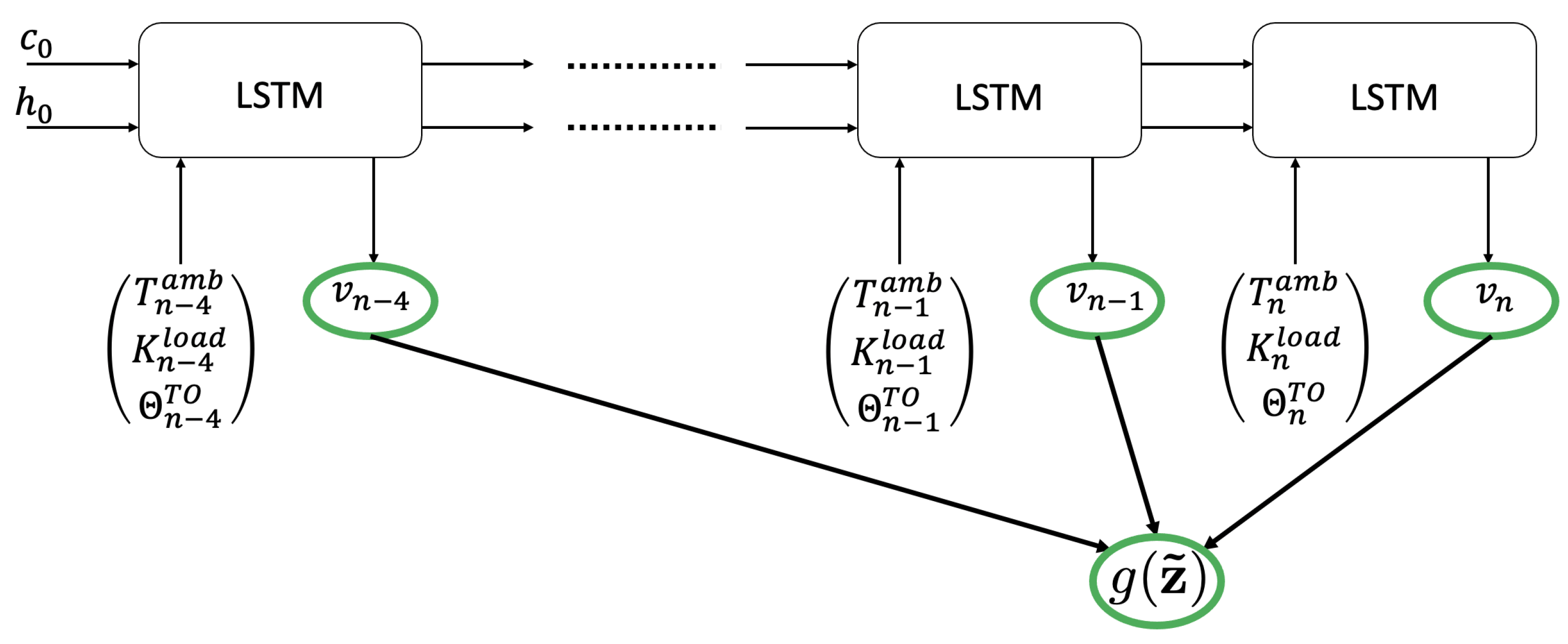
The neural network architecture considered for describing functions

g (\tilde{z})

and

h (\tilde{z})

are both based on the use of LSTM layers combined with a deep dense neural network layer, as described in Table 1 and Table 2 for the linearized ResNet. They were built-up by using Tensorflow Keras libraries. The inputs involved in Eq. (49) are shown in Figure 7.

The training was performed on the initial

80 %

of the available measures, while the testing was performed on the remaining

20 %

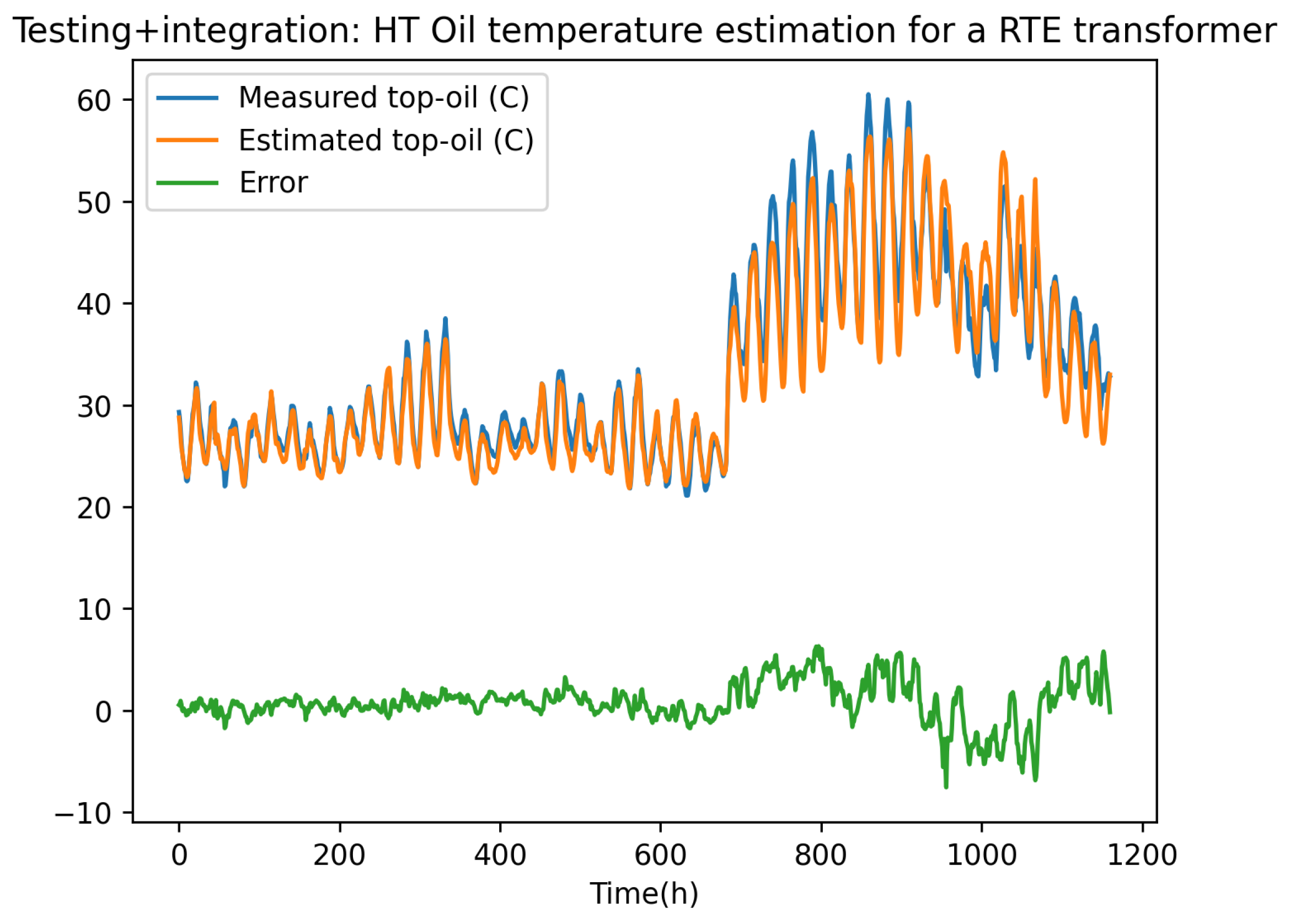
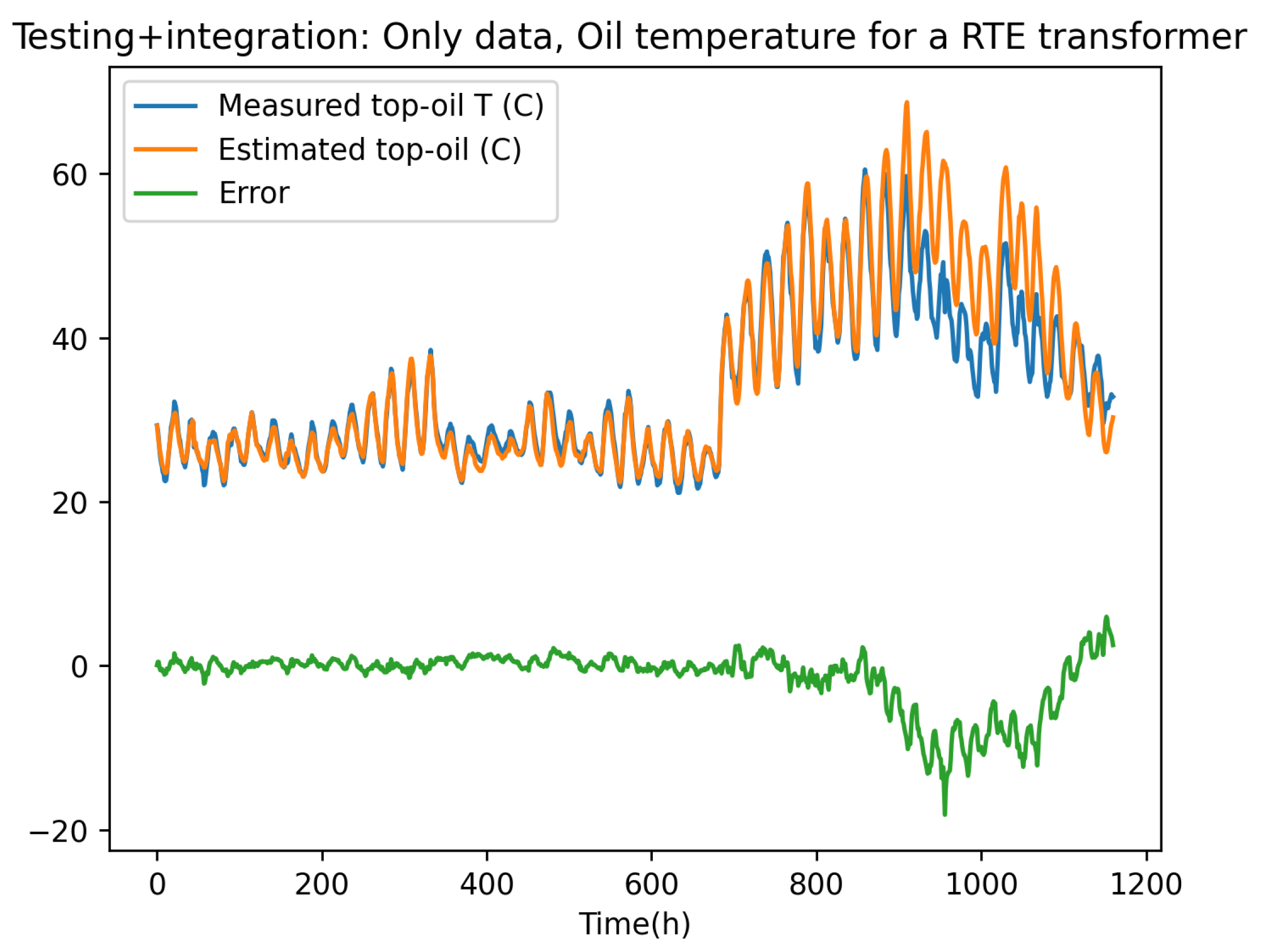
The prediction performed from the corrected (enriched) model is depicted in Figure 8, on the testing interval. It is important to note, that the learnt models

g (\tilde{z})

and

h (\tilde{z})

, were used to integrate the dynamical problem that governs the time evolution of the deviation, Eq. (49), that is, the computed deviation at time

t_{i}

was computed from the one at time

t_{i - 1}

, and then it served to compute the one at the next time step

t_{i + 1}

, and so on.

To distinguish between the known deviation

d (t)

and the one computed from the integrator based on the learnt dynamics

g (\tilde{z})

and

h (\tilde{z})

, the later will be noter by the hat symbol, i.e.

{\hat{d}}_{n + 1} = Δ t g (\tilde{z}) {\hat{d}}_{n} + Δ t h (\tilde{z}) + {\hat{d}}_{n}

(50)

From the computed correction, the model was enriched, exhibiting excellent accuracy and the stability performances.

The fact that the linearized dynamical system operating on the solution correction exhibits good performances, proves that most of the problem nonlinearities were captured by the first order simplified model. When it comes to the nonlinear version of the correction effort, the dynamic version of the model is written in a similar manner as shown in equation (49), with the dynamical integration form used:

{\hat{d}}_{n + 1} = Δ t g (\tilde{z}, {\hat{d}}_{n}) {\hat{d}}_{n} + Δ t h (\tilde{z}) + {\hat{d}}_{n}

(51)

To compare the performances of the hybrid model (data-driven enrichment of the simplified physics-based model), the model governing the experimental data evolution was learnt using the same rationale but now applied on the data, according to:

\{\begin{matrix} Θ_{n + 1} = Δ t g^{θ} (z) Θ_{n} + Δ t h^{θ} (z) + Θ_{n} \\ z = (\begin{matrix} T_{n - 4}^{a m b} & K_{n - 4}^{l o a d} \\ T_{n - 3}^{a m b} & K_{n - 3}^{l o a d} \\ ⋮ \\ T_{n}^{a m b} & K_{n}^{l o a d} \end{matrix}) \end{matrix},

(52)

where

g^{θ} (z)

and

h^{θ} (z)

refer to the parametric functions related to the measured oil temperature, both them depending exclusively on the input features

z

Again, the training was performed using the same model presented in Table 1 and Table 2, with the same

80 %

and

20 %

training and test data-sets.

Figure 9 depicts the results obtained from the integration, where again the hat symbol refers the integrated temperature.

{\hat{Θ}}_{n + 1} = Δ t g^{θ} (z) {\hat{Θ}}_{n} + Δ t h^{θ} (z) + {\hat{Θ}}_{n} .

(53)

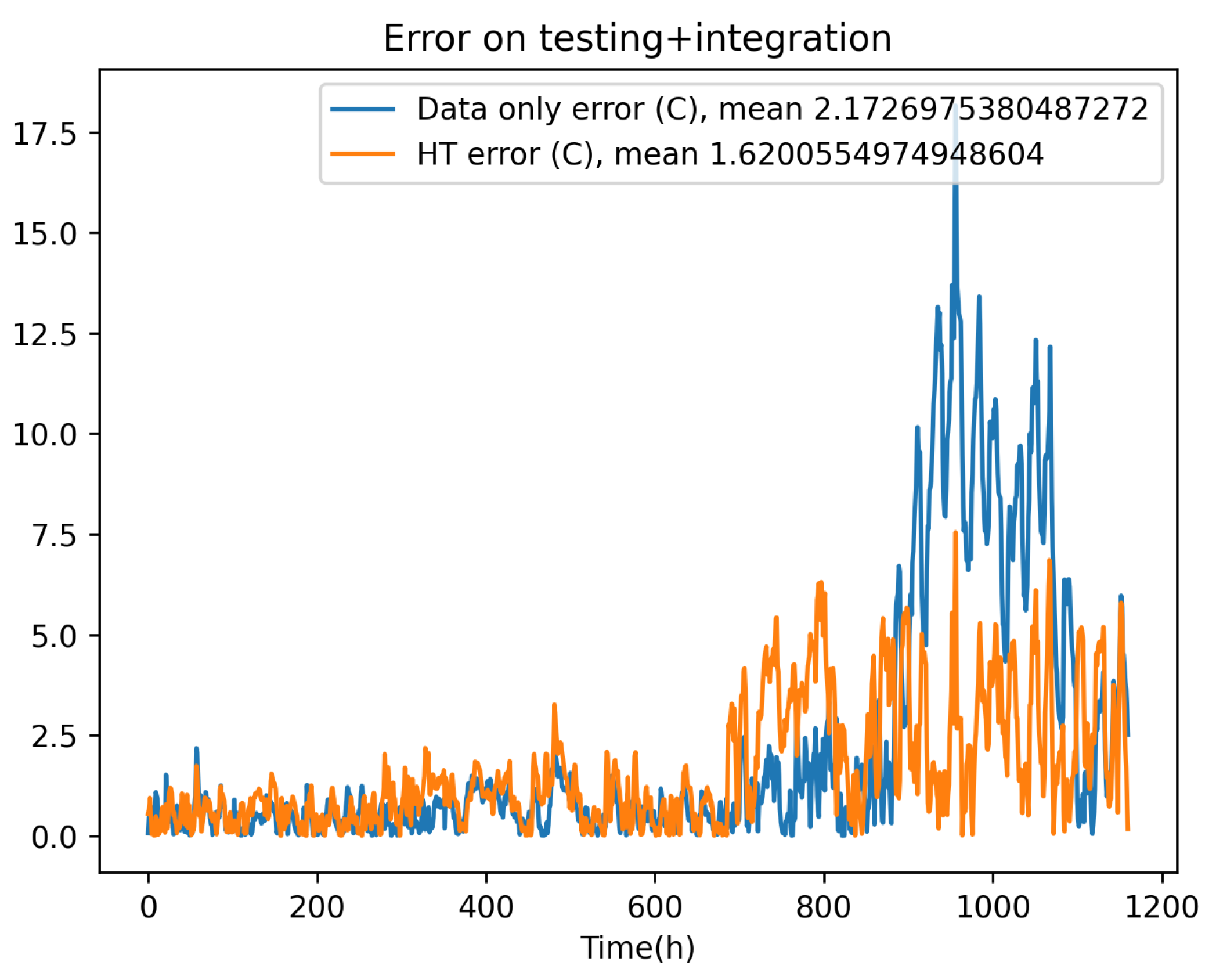
Figure 9 depicts the data-driven model integration, proving the stability performances. However, when comparing the residual error (with respect to the experimental data) of the fully data-driven prediction and the one related to the physics-based enriched solution obtained from the data-driven model of the deviation, both compared in Figure 10, the hybrid modeling framework performs better, ensuring higher accuracy.

Table 3, compares the mean value of the errors associated with the different tested models. From Table 3, one can infer that:

The hybrid approach improves the physics-based model performances.
Enriching a richer nonlinear physics-based model outperform with respect to enriching the linear counterpart of the simplified physics-based model.
When the considered physics-based models are too far from the reference solution (experimental data) the data-driven model can outperform the hybrid modeling.

Table 3. Comparing different built models: mean error (in °C) on the testing set. The nonlinear physics-based model mean error was 3.91°C when used alone, over the same testing set, and 3.25°C for the linear physics based model.

ResNet	Fully	HT from a linear	HT from a nonlinear
	data-driven	physical model	physical model
Linear stabilized	2.173	3.143	1.620
Nonlinear stabilized	1.716	1.516	1.439

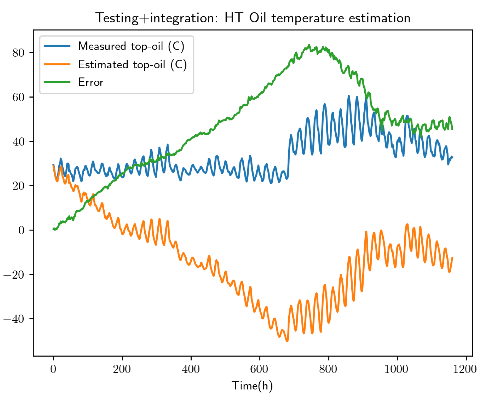
To show the effect of the stabilization, a ResNet is trained without enforcing the stability constraints previously proposed, by using the formulation:

\frac{\partial d}{\partial t} = g (\tilde{z}, d) + h (\tilde{z}),

(54)

with no conditions imposed during the calculation of g and h.

The discrete form

{\hat{d}}_{n + 1} = Δ t g (\tilde{z}, d_{n}) + Δ t h (\tilde{z}) + d_{n},

(55)

provides excellent predictions. It is important note that here the solution at time

t_{n + 1}

{\hat{d}}_{n + 1}

, is computed from the exact deviation at time

t_{n}

d_{n}

However, a full integration where

{\hat{d}}_{n + 1}

is computed from the previously computed

{\hat{d}}_{n}

{\hat{d}}_{n + 1} = Δ t g (\tilde{z}, {\hat{d}}_{n}) + Δ t h (\tilde{z}) + {\hat{d}}_{n},

(56)

produces extremely bad predictions, a direct consequence of the lack of stability.

Figure 11 proves the importance of using stable formulations when the learnt model is expected serving for performing integrations from an initial condition, as it is always the case in prognosis applications.

6. Conclusion

The present paper proposed a hybrid framework where the data-driven model serves to enrich a physics-based model considered as a first approximation of the addressed physics.

We proved that the hybrid framework enhances the predictions accuracy with respect to the physics-based model, however, the hybrid approach is superior to a fully data-driven model only under certain conditions.

The learning technique employed to model the time evolution of the deviation (or the one of the data) must ensure the integration stability. A stabilization has been proposed and its performance proved.

The application to a problem of practical relevance proved the excellent performances of the proposed methodology.

Author Contributions

Conceptualization, F.C.; methodology, C.G. and V.C; software, C.G. and V.C.; validation, X.K. and G.D..; resources, G.D.; writing—original draft preparation, C.G. and F.C.; writing—review and editing, C.G., F.C. and X.K.; supervision, X.K. and G.D.; project administration, G.D. All authors have read and agreed to the published version of the manuscript.

Funding

This research received no external funding

Data Availability Statement

Data could be available under request to the authors, after agreement of RTE.

Acknowledgments

Authors acknowledge the support of the RTE, SKF and ESI research chairs at Arts et Métiers institute of technology.

Conflicts of Interest

The authors declare no conflict of interest.

Sample Availability

Samples of the compounds ... are available from the authors.

References

C. Argerich, A. Carazo, O. Sainges, E. Petiot, A. Barasinski, M. Piana, L. Ratier, F. Chinesta. Empowering Design Based on Hybrid Twin: Application to Acoustic Resonators. Designs, 4, 44, 2020. [CrossRef]
P.C. Blaud, P. Chevrel, F. Claveau, P. Haurant, A. Mouraud. Resnet and polynet based identification and (mpc) control of dynamical systems: a promising way. IEEE Access, 11, 20657-20672, 2022.
D. Borzacchiello, J.V. Aguado, F. Chinesta. Non-intrusive sparse subspace learning for parametrized problems. Archives of Computational Methods in Engineering, 26, 303-326, 2019.
L. Breiman. Random Forests. Machine Learning 45, 5-32, 2001.
F. Casteran, K. Delage, P. Cassagnau, R. Ibanez, C. Argerich, F. Chinesta. Application of Machine Learning tools for the improvement of reactive extrusion simulation. 2020. [CrossRef]
F. Chinesta, E. Cueto, E. Abisset-Chavanne, J.L. Duval, F. El Khaldi, Virtual, Digital and Hybrid Twins: A New Paradigm in Data-Based Engineering and Engineered Data, Archives of Computational Methods in Engineering, 27, 105-134, 2020.
R.T.Q. Chen, Y. Rubanova, J. Bettencourt, D. Duvenaud. Neural ordinary differential equations. Conference on Neural Information Processing Systems (NeurIPS 2018), Vol. 32, Montreal, Canada, 1-18, 2018.
R.T.Q. Chen, B. Amos, M. Nickel. Learning Neural Event Functions for Ordinary Differential Equations, 2020 https://arxiv.org/abs/2011.03902.
N. Cristianini, J. Shawe-Taylor. An introduction to support vector machines and other kernel-based learning methods. Cambridge University Press, New York, 2000.
S.H. Dar, W. Chen, F. Zheng, S. Gao, K. Hu. An LSTM with Differential Structure and Its Application in Action Recognition, Mathematical Problems in Engineering, 2022, 7316396, 2022.
G.P. Distefano. Stability of numerical integration techniques. AIChE Journal, 14(6), 946-955, 1968.
L. Enciso-Salas, G. Perez-Zuniga, J. Sotomayor-Moriano. Fault Detection and Isolation for UAVs using Neural Ordinary Differential Equations. IFAC-PapersOnLine, 55(6), 643-648, 2022.
R. Ghanem, C. Soize, L. Mehrez, V. Aitharaju. Probabilistic learning and updating of a digital twin for composite material systems, IJNME, 2020. [CrossRef]
C. Ghnatios, P. Gérard, A. Barasinski. An advanced resin reaction modeling using data-driven and digital twin techniques. International Journal of Material Forming, 16, 5, 2023.
D. Gonzalez, F. Chinesta, E. Cueto. Learning corrections for hyper-elastic models from data. Frontiers in Materials - section Computational Materials Science, 6, 2019.
I. Goodfellow, Y. Bengio, A. Courville. Deep learning. MIT Press, Cambridge, 2016.
K. He, X. Zhang, S. Ren, J. Sun. Deep residual learning for image recognition. IEEE Conference on Computer Vision and Pattern Recognition (CVPR), Las Vegas, NV, USA, 770-778, 2016.
K. He, X. Zhang, S. Ren, J. Sun. Identity Mappings in Deep Residual Networks. In: Leibe, B., Matas, J., Sebe, N., Welling, M. (eds) Computer Vision - ECCV 2016. ECCV 2016. Lecture Notes in Computer Science, Vol 9908. Springer, Cham, 2016.
S. Hochreiter, J. Schmidhuber. Long Short-Term Memory. Neural Computation 9(8), 1735-1780, 1997.
R. Ibanez, E. Abisset-Chavanne, D. Gonzalez, J.L. Duval, E. Cueto, F. Chinesta. Hybrid Constitutive Modeling: Data-driven learning of corrections to plasticity models. International Journal of Material Forming, 12, 717-725, 2019.
M.G. Kapteyn, K.E. Willcox. From Physics-Based Models to Predictive Digital Twins via Interpretable Machine Learning, 2020 arXiv:2004.11356v3.
X. Kestelyn, G. Denis, V. Champaney, N. Hascoet, C. Ghnatios, F. Chinesta. Towards a hybrid twin for infrastructure asset management: Investigation on power transformer asset maintenance management. 7th International Advanced Research Workshop on Transformers (ARWtr), 109-114, 2022.
C.W. Kirkwood. Decision Tree primer, 2002, http://creativecommons.org/licenses/by-nc/3.
B. Moya, A. Badias, I. Alfaro, F. Chinesta, E. Cueto. Digital twins that learn and correct themselves. International Journal for Numerical Methods in Engineering. [CrossRef]
G. Quaranta, M. Ziane, E. Haug, J.L. Duval, F. Chinesta. A minimally-intrusive fully 3D separated plate formulation in computational structural mechanics. Advanced Modelling and Simulation in Engineering Sciences, 6, Article number 11, 2019.
A. Reille, V. Champaney, F. Daim, Y. Tourbier, N. Hascoet, D. Gonzalez, E. Cueto, J.L. Duval, F. Chinesta. Learning data-driven reduced elastic and inelastic models of spot-welded patches. Mechanics & Industry, 22, 32, 2021.
A. Sancarlos, M. Cameron, A. Abel, E. Cueto, J.L. Duval, F. Chinesta. From ROM of electrochemistry to AI-based battery digital and hybrid twin. Archives of Computational Methods in Engineering, 28, 979-1015, 2021.
A. Sancarlos, J.M. Le Peuvedic, J. Groulier, J.L. Duval, E. Cueto, F. Chinesta. Learning stable reduced-order models for hybrid twins. A. Sancarlos, M. Cameron. Data Centric Engineering, 2, e10, 2021.
A. Sancarlos, V. Champaney, E. Cueto, F. Chinesta. Regularized regressions for parametric models based on separated representations. Advanced Modeling and Simulation in Engineering Sciences, 10:4, 2023. [CrossRef]
P.J. Schmid. Dynamic mode decomposition of numerical and experimental data. J Fluid Mech., 656, 528, 2010.
J. Schmidhuber. Deep learning in neural networks: An overview. Neural Networks. 61, 85-117, 2015.
B. Settles, Active Learning Literature Survey. Computer Sciences Technical Report 1648. University of Wisconsin-Madison, 2009.
Standard. Loading guide for mineral-oil-immersed power transformers. International electrotechnical commission, 3, rue de Varembé, PO Box 131, CH-1211 Geneva 20, Switzerland, 1, 2018.
S. Torregrosa, V. Champaney, A. Ammar, V. Hebert, F. Chinesta. Surrogate Parametric Metamodel based on Optimal Transport. Mathematics and Computers in Simulation, 194, 36-63, 2022.
S. Torregrosa, V. Champaney, A. Ammar, V. Herbert, F. Chinesta. Hybrid Twins based on Optimal Transport. Computers and Mathematics with Applications, 127, 12-24, 2022.
E.J. Tuegel, A.R. Ingraffea, T.G. Eason, S.M. Spottswood. Reengineering Aircraft Structural Life Prediction Using a Digital Twin. International Journal of Aerospace Engineering, 154798, 2011.
G.B. Zhou, J. Wu, C.L. Zhang, Z.H. Zhou. Minimal gated unit for recurrent neural networks. International journal Automation and Computing, 13, 226-234, 2016.

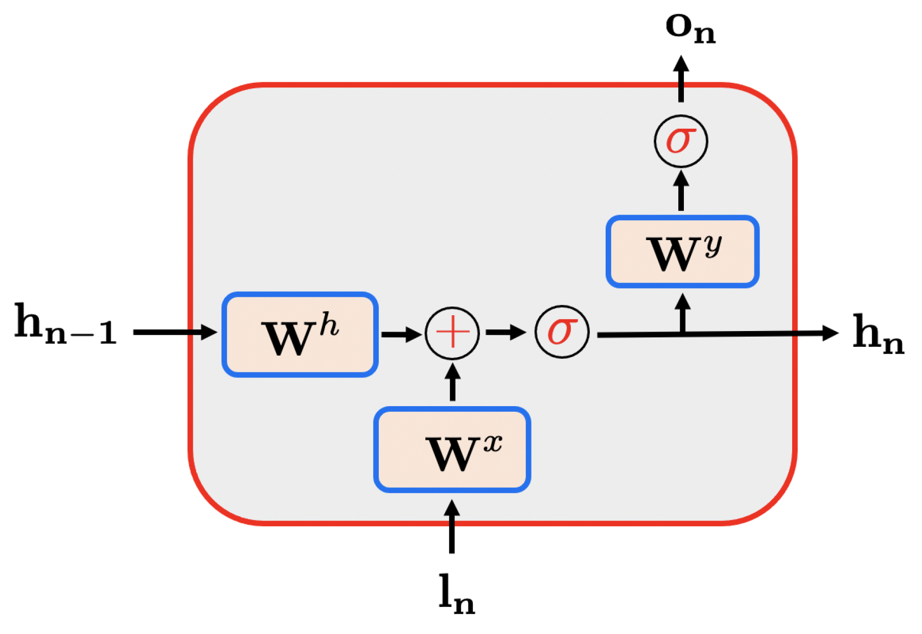
Figure 1. Recurrent Neural Network architecture.

Figure 2. LSTM-block architecture: The output

o_{n}

results from

l_{n}

the previous

m - 1

inputs while it almost totally forget the initial hidden long and short memory states

h_{0}

and

c_{0}

that can be initialized with zero values.

Figure 2. LSTM-block architecture: The output

o_{n}

results from

l_{n}

the previous

m - 1

inputs while it almost totally forget the initial hidden long and short memory states

h_{0}

and

c_{0}

that can be initialized with zero values.

Figure 3. ResNet global architecture and integration mode (dotted line).

Figure 4. Solution computed by integrating the linear (top) and nonlinear (bottom) learning procedures.

Figure 5. Solution computed by integrating the linear (top) and nonlinear (bottom) learning procedures.

Figure 6. Experimental data

Θ (t)

, simulated solution

Θ^{T O} (t)

and deviation

d (t) = Θ (t) - Θ^{T O}

Figure 6. Experimental data

Θ (t)

, simulated solution

Θ^{T O} (t)

and deviation

d (t) = Θ (t) - Θ^{T O}

Figure 7. Network considered to model

g (\tilde{z})

. Variables

v_{i}

are intermediate variables, involved in the construction of

g (\tilde{z})

. A similar architecture is considered for modeling

h (\tilde{z})

Figure 7. Network considered to model

g (\tilde{z})

. Variables

v_{i}

are intermediate variables, involved in the construction of

g (\tilde{z})

. A similar architecture is considered for modeling

h (\tilde{z})

Figure 8. Physics-based simplified model correction from a stabilized linearized ResNet model, here illustrated on the test data-set.

Figure 9. Full data-driven model consisting on a stabilized ResNet model, here illustrated on the test data-set.

Figure 10. Comparing the errors of the data-only linearized ResNet and the linearized ResNet hybrid model, on the test data-set.

Figure 11. Integration performed from a ResNet learnt without enforcing stability constraints.

Table 1. The building blocks of the LSTM-based surrogate of

g (\tilde{z})

Table 1. The building blocks of the LSTM-based surrogate of

g (\tilde{z})

Layer	Building block	Activation
1	LSTM layer with 5 outputs, return sequence true	$s i g m o i d$ + $t a n h$
2	Flatten	No activation
3	Dense connection with 1 output	$r e l u$
4	Lambda layer returning $- 1 \times i n p u t s$	No activation

Table 2. The building blocks of the LSTM-based surrogate of

h (\tilde{z})

Table 2. The building blocks of the LSTM-based surrogate of

h (\tilde{z})

Layer	Building block	Activation
1	LSTM layer with 5 outputs, return sequence true	$s i g m o i d$ + $t a n h$
2	Flatten	No activation
3	Dense connection with 1 output	$L i n e a r$

Disclaimer/Publisher’s Note: The statements, opinions and data contained in all publications are solely those of the individual author(s) and contributor(s) and not of MDPI and/or the editor(s). MDPI and/or the editor(s) disclaim responsibility for any injury to people or property resulting from any ideas, methods, instructions or products referred to in the content.

© 2023 by the authors. Licensee MDPI, Basel, Switzerland. This article is an open access article distributed under the terms and conditions of the Creative Commons Attribution (CC BY) license (http://creativecommons.org/licenses/by/4.0/).

Copyright: This open access article is published under a Creative Commons CC BY 4.0 license, which permit the free download, distribution, and reuse, provided that the author and preprint are cited in any reuse.

MDPI Initiatives

Important Links

Choose an area of interest and we will send you notifications of new preprints at your preferred frequency.

Disclaimer

Learning Data-Driven Stable Corrections of Dynamical Systems. Application to the Simulation of the Top-Oil Temperature Evolution of a Power Transformer

Abstract

1. Introduction

1.1. The three main SBE methodologies revisited

2. Illustrating the hybrid approach

2.1. A simple linear regression reasoning

2.2. General remarks

2.3. On the domain of application of the hybrid modeling approach

3. Methods

3.1. On the integration stability

3.2. Learning integrators

3.2.1. Recurrent Neural Network

3.2.2. On the model memory

3.2.3. Learners with larger memory

3.2.4. Residual Nets

4. Simple procedures for stabilizing ResNets-based integration

4.1. Learning stable linear dynamical systems

4.2. Learning stable nonlinear dynamical systems

4.3. Numerical examples and discussion

4.3.1. Linear dynamical system

4.3.2. Nonlinear dynamical system

4.4. Final remarks

5. Application to the evaluation of the top-oil temperature of an electric power transformer

6. Conclusion

Author Contributions

Funding

Data Availability Statement

Acknowledgments

Conflicts of Interest

Sample Availability

References

MDPI Initiatives

Important Links

Subscribe