1. Introduction
Consider the following linear equation systems:
with
is a convex combination Google matrix composed of matrix
P and matrix
E, and
, where
denotes the damping factor that determines the weight given to the web link graph, and
,
, and
is a personalization vector or a teleportation vector.
n is the dimension of
P, and
x is our desired eigenvector.
The system of linear equations in (1.1) above is what we refer to as the PageRank problem. Google’s PageRank algorithm has grown to be one of the most well-known algorithms in online search engines thanks to the rapid development of the internet, link analysis method called PageRank is used to rank online pages and assess their significance in relation to the link structure of Web, calculating the primary eigenvectors of the Google matrix, forms the basis of the PageRank algorithm. Although Google’s exact ranking technology and calculation techniques have gradually improved, the PageRank problem is still a major concern and has recently gained a lot of attention in the world of scientific and engineering computation.
To solve the PageRank problem, the power method is easy to calculate and the most classical algorithm, while all other eigenvalues of matrix
aside from the principal eigenvalues are simply scalar times the corresponding eigenvalues of matrix
P. As a result, the power approach converges very slowly when the primary eigenvalue of matrix
is closely related to other eigenvalues, or when the damping factor is close to 1. The power method is not the ideal way to solve this problem, but a quicker and more logical way to solve the principal eigenvectors of the Google matrix is required to speed up the calculation of PageRank. The network graph is extremely large, with 1 billion or even 10 billion web page nodes. Additionally, a good search algorithm should minimize the lag time, which is the time from the search target proposed to the search result feedback to the web browser. In recent years, numerous researchers have proposed various methods to speed up the calculation of PageRank, among them, the design of power function method and its variant method for accelerating the solution of PageRank problem are favored by many researchers. For instance, Gleich et al. [
4] proposed an inner outer iteration method combined with Richardson iteration, in which each iteration needs to solve a linear system whose algebraic structure is similar to the original system; Gu and Xie [
5] proposed the PIO iteration algorithm, which combines the power method and the inner-outer iteration method, after that, Ma et al. [
11] suggested a relaxed two-step splitting iteration strategy to address the PageRank problem based on [
4] and [
5], adding a new relaxation parameter; Gu et al. [
8] introduced a two parameter iteration approach based on multiplicative splitting iteration in order to increase the possibility of optimizing the iterative process; based on the iteration framework [
7] and relaxed two-step splitting (RTSS) iteration method [
11], Two relaxed iteration techniques are presented by Tian et al. [
12] for resolving the PageRank issue. Additionally, the PageRank problem can be solved by using Krylov subspace methods, which is a problem of solving linear equations. For instance, Wu and Wei propose a hybrid algorithm, power-Arnoldi algorithm [
14], which combines its power technique and thick restart Arnoldi algorithm; as well as the Arnoldi-extrapolation method [
26] and speeding the Arnoldi-type algorithm [
23]. We cite [
7,
8,
9,
10,
11,
12,
13,
14,
15,
16,
17,
18,
19,
20,
21,
22,
23,
24,
25,
26,
27,
28,
29] for a more in-depth theoretical study.
The structure of this essay is as follows: we briefly introduce the inner-outer iterative PageRank problem techniques in
Section 2. In
Section 3, we first examine the theoretical foundations of the multiplicative splitting iterative method before introducing our brand-new approach, the parameterized MSI iteration method.
Section 4 reports on numerical testing and comparisons. Finally,
Section 5 provides a few succinct closing notes.
2. The inner-outer method
First, we provide a brief summary of the methodological inside-out iteration procedure proposed by Gleich et al. [
4], for computing the inside-out iteration of PageRank. It is clear that linear systems can be used to rewrite the eigenvector problem (1.1).
since
We observe that when the damping vector is small, it is simpler to solve the PageRank problem, Gleich et al. defined the outer iteration with a smaller damping factor
(
), rather than immediately resolving the equation (1.1). Therefore, the equations below are used to rewrite the linear system (1.1).
So the stationary outer iteration scheme
For computing
, define the inner linear system as
where
, and compute
via the Richardson inner iteration
where
, The
l-th step inner solution
is assigned to be the next new
. The stopping criteria are given as follows, The outer iteration (2.1) terminates if
while the inner iteration (2.5) terminates if
where
and
are the inner and outer tolerances respectively.
The MSI iteration method
Gu et al. suggested the MSI approach in [
8] to expedite the PageRank vector calculation. Here is a quick overview of the MSI approach, the MSI approach entails writing
as
here
, given an initial vector
, for
, perform the following two-step iteration
until the sequence
converges to the exact solution
.
Theorem 2.1 ([
8])
. Let α be the damping factor in the PageRank linear system, and let , are the two splittings of the matrix . Then the iterative matrix of the MSI method for PageRank computation is given by
and its spectral radius is bounded by
therefore, it holds that
the multiplicative splitting iteration method for PageRank computation converges to the unique solution of the linear system of equations.
3. The parameterized MSI iteration method
The PageRank problem model is presented in this section, and it illustrates how the problem can be solved more simply by choosing a smaller damping factor . We introduce a parameter based on the MSI method in order to further control the range of , reduce the spectral radius, and speed up convergence, this results in a new iterative algorithm, denoted as the PMSI method below, that is described as follows.
The PMSI iteration method
with
and
,
. If
, then the PMSI iteration method becomes the MSI iteration method.
|
Algorithm 1:PMSI method |
-
Input:
Parameters P, q, v, , , ; - 1:
-
Output:
x - 2:
- 3:
- 4:
- 5:
ifthen
- 6:
- 7:
; - 8:
- 9:
repeat
- 10:
- 11:
; - 12:
- 13:
; - 14:
- 15:
until
- 16:
- 17:
; - 18:
- 19:
repeat
- 20:
- 21:
; - 22:
- 23:
; - 24:
- 25:
until
- 26:
- 27:
; - 28:
- 29:
; - 30:
- 31:
end if - 32:
- 33:
. |
Remark 3.1. The computational cost of the PMSI iteration approach is somewhat higher than that of (2.8) since it simply requires an additional saxpy operation, Vector addition and the price each iteration of with flops.
In the sequel, we will analyze the convergence property of the parameterized MSI iteration method.
Lemma 3.1 ([
8])
. Let , be two splittings of the matrix , and let be a given initial vector. If is a two-step iteration sequence
then
Moreover, if the spectral radius is less than 1, then the iteration sequence converges to the unique solution of the system of linear equation (2.1) for all initial vectors .
The multiplicative splitting iteration method for (2.1) is obviously related with the splitting of the coefficient matrix
, and we will subsequently demonstrate that there exists a plausible convergent domain of two-parameters for the parameterized method.
according to (3.1), The two-step iterative matrix corresponding to the multiplication split iterative method is as follows
Now, we examine the convergence property of the multiplicative-splitting iterative method. By applying Lemma 3.1, we can obtain the following main theorem..
Theorem 3.1.
Let α be the damping factor in the PageRank linear system, and let , are the two splittings of the matrix . Then the iterative matrix of the PMSI method for PageRank computation is given by
and its spectral radius is bounded by
therefore, it holds that
the multiplicative splitting iteration method for PageRank computation converges to the unique solution of the linear system of equations.
Proof. From Lemma 3.1 we can obtain the iterative matrix of the PMSI method for PageRank computation Eq. (3.5)).
Let , since , , then the matrix is a nonnegative matrix and the matrix is also nonnegative.
In addition, from (3.5) it turns out that
if
is an eigenvalue of
P, The spectral radius of
are
for
Since
, combining the above relations (3.9) and (3.10), we can get
So for any given constants and , . The PMSI method converges to a unique solution to the linear system (2.1), the PageRank vector. □
Since , then . Immediately, a comparison result is obtained for the parameterized MSI iteration method compared with the MSI iteration method.
Theorem 3.2. Let , , If , then the parameterized MSI iteration method converges faster than the MSI iteration method.
Proof. From Eq (3.9), it follows that the spectral radius of the parameterized MSI iteration method is
Let
in (3.12), then we obtain the spectral radius of the MSI iteration method as follows:
For
, from (3.12)-(3.13), it is clear that
It is obvious that , and the proof is completed. □
Corollary 3.1. In the range of , , , when ω increases gradually within the value range, the smaller the iterative spectral radius of the PMSI algorithm, the faster the convergence speed.
Proof. According to Equation (3.9), we know that
It is easy one can obtain from above relation
since
,
, so we have
. we can get
, we can see the PMSI iterative method may be more efficient when
is large, the conclusion is proved. □
4. Numerical results
In this section, we compare the performance of the parameterized multisplitting (PMSI) iteration method to that of the inner-outer (IO) and multi-splitting (MSI) iteration methods, respectively. On dual-core processing, numerical experiments are carried out in Matlab R2018a (2.30 GHz, 8GB RAM). Four iteration parameters, the number of matrix vectors (denoted as MV), the iteration step size (denoted as IT), the calculation time in seconds (denoted as CPU), and the relative residual (denoted as res(k)) are used to test these iterative approaches, defined
where
.
Table 1 lists the properties of the test matrices
P, where average non-zero refers to each row of non-zero elements, and
All test matrices can be downloaded from
https://www.cise.ufl.edu/research/sparse/matrices/list_by_id.htmlget. For the interest of fairness, we assume that the transfer vector
(
) is the initial guess for each test matrix. In all numerical tests, the damping factors are assumed to be
0.99,
0.997,
. The residual specification
determines when all algorithms end.
Table 1.
properties of test matrices
Table 1.
properties of test matrices
| |
Size |
|
|
| wb-cs-stanford |
9914×9914 |
2 312 497 |
0.291
|
| amazon0312 |
400,727×400,727 |
3200,440 |
1.993
|
Example 4.1.
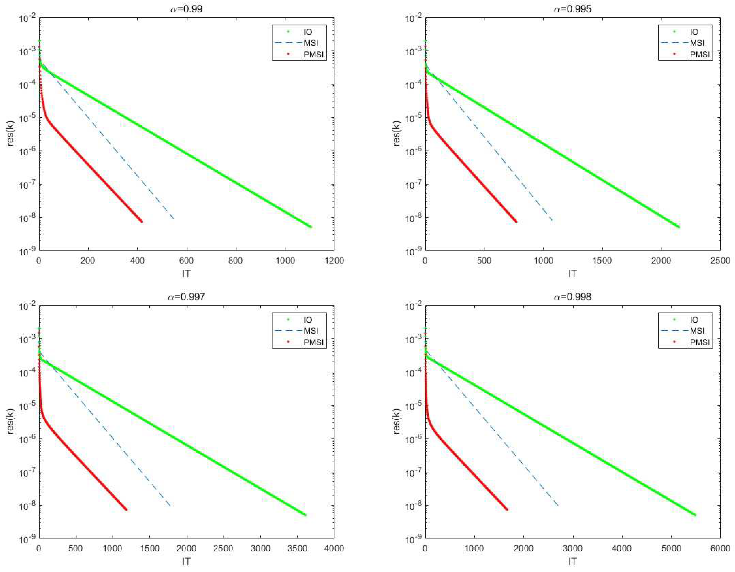
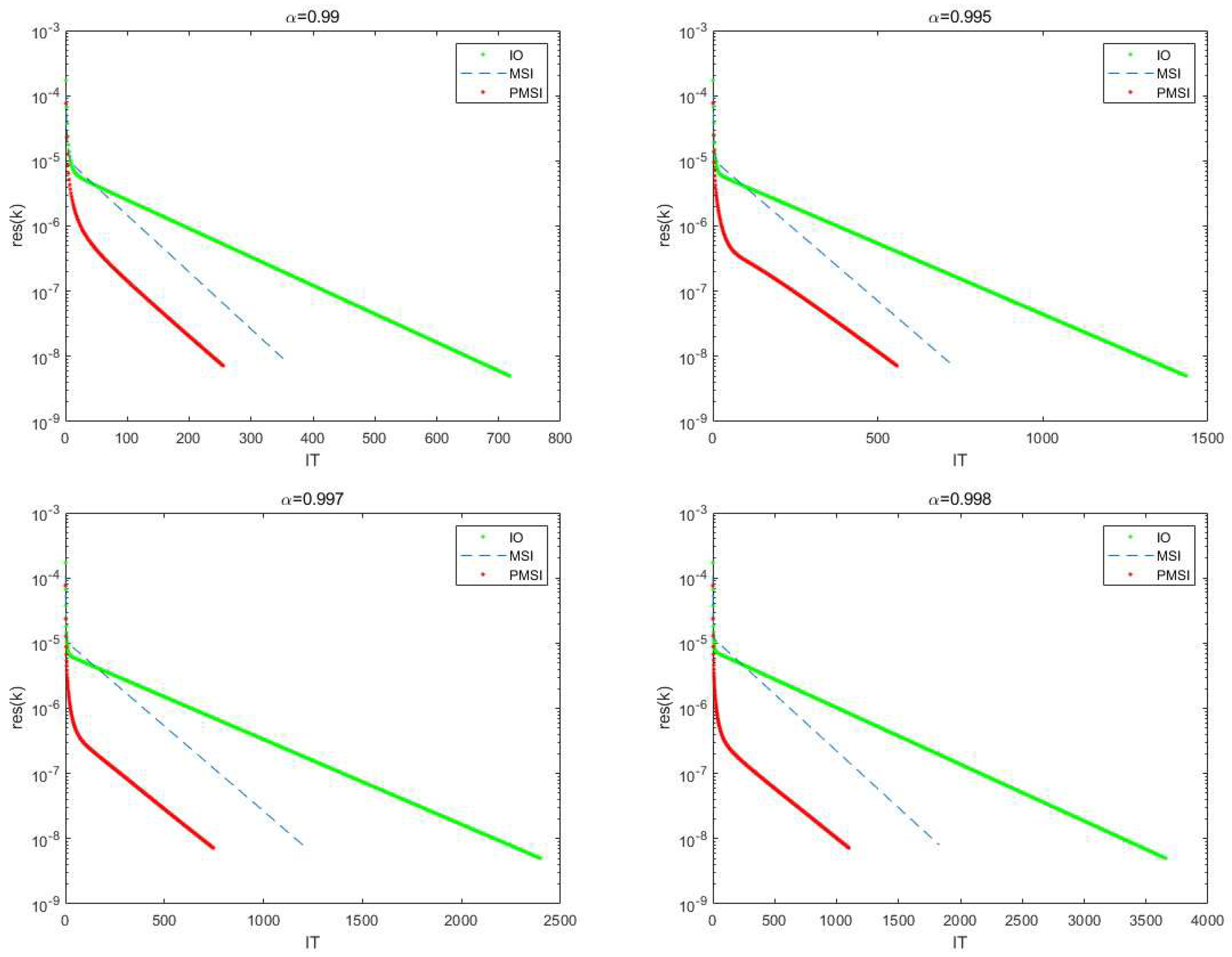
In this example, we compare the PMSI iteration method with the MSI iteration method. The test matrices are the wb-cs-stanford, and amazon0312 matrices, respectively. In order to verify the efficiency of the PMSI iteration method, we use
to describe the speedups of the PMSI iteration compared with the MSI iteration associated with CPU time.
The numerical outcomes of the MSI and PMSI iterative procedures, where and and , are displayed in Tables 2 and 3. Tables 2 and 3 shows that the PMSI iterative technique performs better than the MSI iterative method in terms of IT, MV, and CPU time, especially for bigger α, such the in Tables 2 and 3. As can be observed, most values are more than 20%, sometimes even reaching 50%.
Table 2.
Test results for the wb-cs-stanford matrix
Table 2.
Test results for the wb-cs-stanford matrix
|
|
|
|
|
|
| |
IT(MV) |
536 |
270(541) |
228(457) |
|
| 0.98 |
CPU |
0.1261 |
0.1268 |
0.1079 |
14.90% |
| |
IT(MV) |
1096 |
537(1075) |
417(835) |
|
| 0.99 |
CPU |
0.2151 |
0.2274 |
0.1648 |
27.52% |
| |
IT(MV) |
2168 |
1095(2191) |
962(1525) |
|
| 0.995 |
CPU |
0.7280 |
0.3819 |
0.2942 |
22.96% |
| |
IT(MV) |
3577 |
1806(3613 ) |
1213(2427) |
|
| 0.997 |
CPU |
0.6380 |
0.5954 |
0.4350 |
26.93% |
| |
IT(MV) |
5450 |
2698(5397) |
1663(3327) |
|
| 0.998 |
CPU |
0.9354 |
0.8669 |
0.5862 |
32.37% |
Table 3.
Test results for the amazon0312 matrix
Table 3.
Test results for the amazon0312 matrix
|
|
|
|
|
|
| |
IT(MV) |
367 |
178(357) |
170(341) |
|
| 0.98 |
CPU |
7.3867 |
6.8073 |
6.5658 |
3.54% |
| |
IT(MV) |
733 |
363(727) |
292(585) |
|
| 0.99 |
CPU |
15.7108 |
14.1045 |
12.0670 |
14.44% |
| |
IT(MV) |
1436 |
723(1447) |
5110(1021) |
|
| 0.995 |
CPU |
30.1137 |
29.4107 |
21.2650 |
27.69% |
| |
IT(MV) |
2507 |
1164(2329) |
717(1435) |
|
| 0.997 |
CPU |
30.1137 |
48.6659 |
27.8410 |
42.79% |
| |
IT(MV) |
3630 |
1863(3727) |
911(1823) |
|
| 0.998 |
CPU |
90.7846 |
75.3888 |
37.6927 |
50.00% |
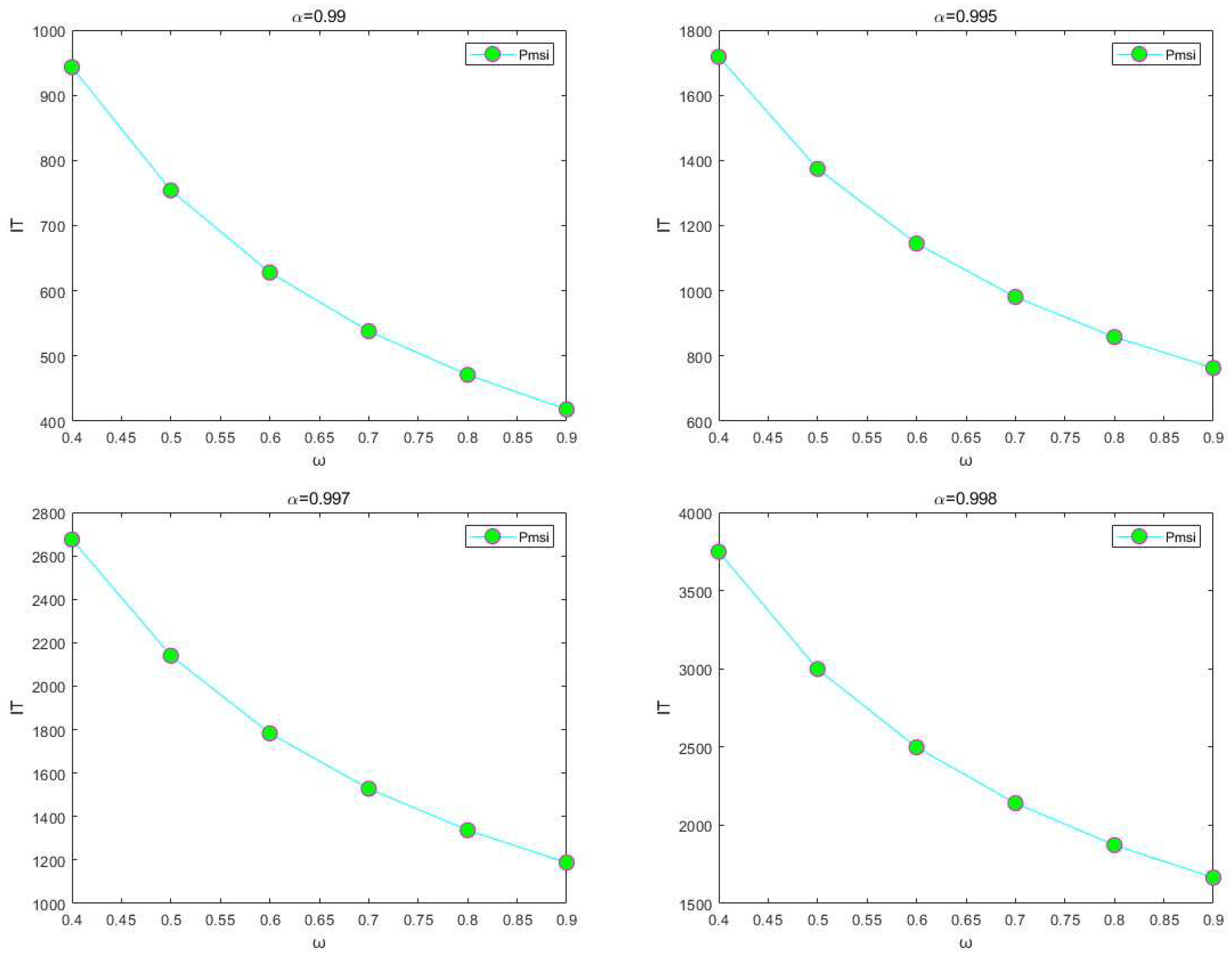
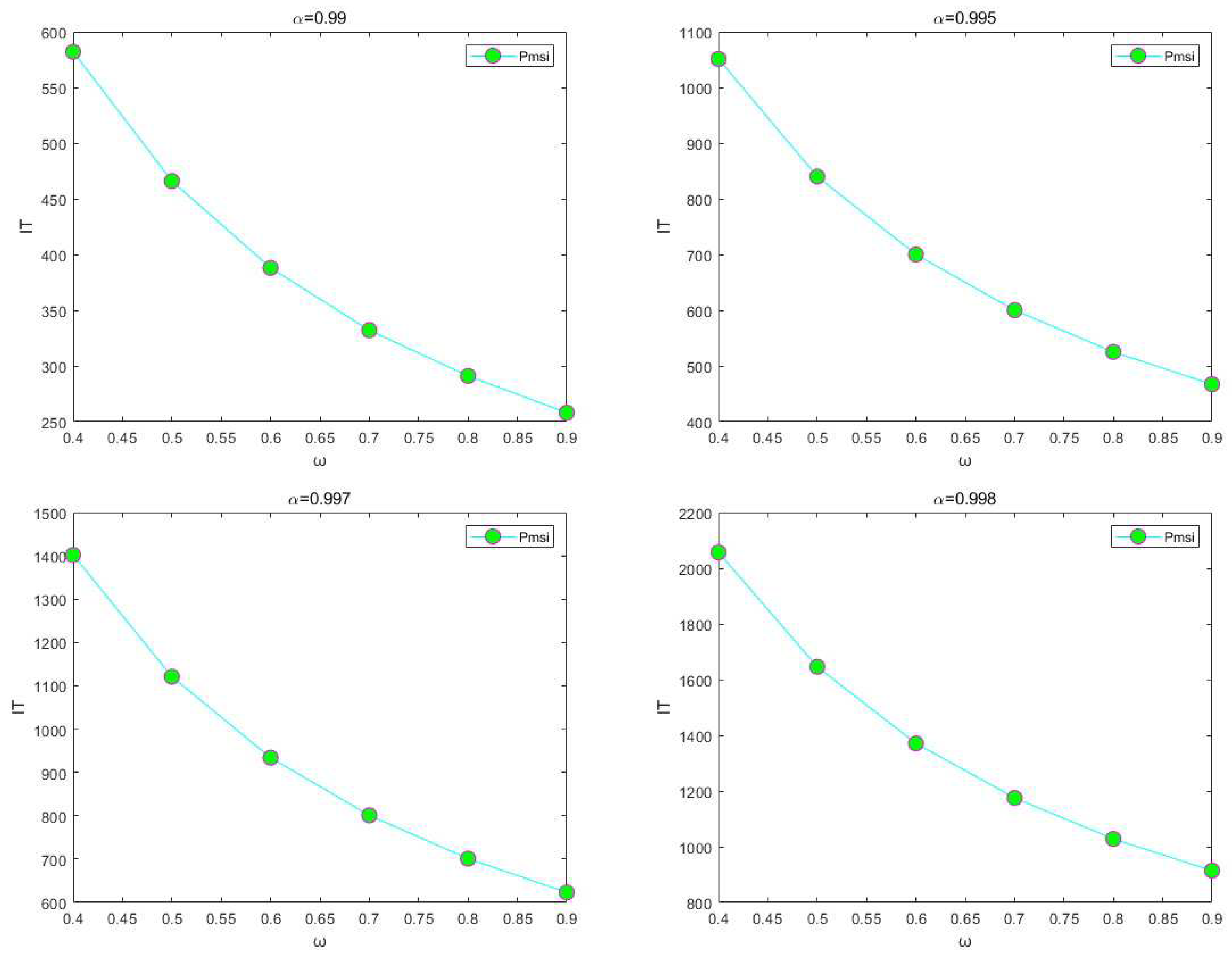
Example 4.2. With the test matrices being the wb-cs-stanford and amazon0312 matrix with various ω parameters, we will further examine the convergence performance of the PMSI iterative method in this example. We have set the ω value range to . The numerical outcomes are shown in Figure 3, where and . According to the findings, the number of repetitions constantly lowers as ω rises. Because of this, we used ω = 0.9 in our studies, which is consistent with the finding in Corollary 3.1.
Example 4.3. Theorem 3.1 states that the PMSI method converges for any value of and , satisfying the conditions of and . This is what we take into consideration in this example. For two matrices, wb-cs-stanford and amazon0312, Tables 4 and 5 display the number of iterations of the PMSI approach. The values of and change from 0.1 to 0.9 and 0.1 to 0.9, respectively, when α = 0.99. From Tables 4 and 5, it can be inferred that, once one of the parameters and is determined, the number of iteration steps typically decreases first before increasing as more parameters are added. For instance, in Table 3, increased from of 0.8 to of 0.9. The number of iteration steps first declines, and then takes 0.1 to 0.5, and the number of iteration steps continues to rise. Finding an explicit link between and , or the ideal and , for the universal PageRank matrix, is quite difficult. Our considerable experience has shown that selecting =0.9 and =0.8 usually results in good performance. For this reason, in our studies, we used =0.9 and =0.8 in the PMSI approach.
Figure 1.
Convergence effect of three algorithms for wb-cs-stanford matrix,
Figure 1.
Convergence effect of three algorithms for wb-cs-stanford matrix,
Figure 2.
Convergence effect of three algorithms for amazon0312 matrix,
Figure 2.
Convergence effect of three algorithms for amazon0312 matrix,
Figure 3.
Numerical results for the wb-cs-stanford matrix in Example 4.2
Figure 3.
Numerical results for the wb-cs-stanford matrix in Example 4.2
Figure 4.
Numerical results for the amazon0312 matrix in Example 4.2
Figure 4.
Numerical results for the amazon0312 matrix in Example 4.2
Table 4.
Numerical results for the wb-cs-stanford matrix in Example 4.3
Table 4.
Numerical results for the wb-cs-stanford matrix in Example 4.3
|
0.1 |
0.2 |
0.3 |
0.4 |
0.5 |
0.6 |
0.7 |
0.8 |
0.9 |
| 0.1 |
418(837) |
410(821) |
419(839) |
419(839) |
414(829) |
422(845) |
415(831) |
417(835) |
415(831) |
| 0.3 |
416(833) |
415(831) |
418(837) |
417(835) |
420(841) |
415(831) |
426(853) |
422(845) |
417(835) |
| 0.5 |
412(825) |
420(841) |
415(831) |
416(833) |
425(851) |
411(823) |
426(853) |
424(569) |
418(837) |
| 0.7 |
418(837) |
414(829) |
417(837) |
414(829) |
419(839) |
416(833) |
412(825) |
419(839) |
417(835) |
| 0.9 |
420(841) |
422(845) |
428(857) |
420(841) |
424(849) |
422(845) |
416(833) |
417(835) |
412(825) |
Table 5.
Numerical results for the amazon0312 matrix in Example 4.3
Table 5.
Numerical results for the amazon0312 matrix in Example 4.3
|
0.1 |
0.2 |
0.3 |
0.4 |
0.5 |
0.6 |
0.7 |
0.8 |
0.9 |
| 0.1 |
293(587) |
275(551) |
262(525) |
302(605) |
284(569) |
269(539) |
275(551) |
277(555) |
262(525) |
| 0.3 |
262(525) |
265(531) |
294(589) |
262(525) |
263(527) |
303(607) |
271(543) |
269(539) |
258(517) |
| 0.5 |
281(563) |
257(535) |
269(539) |
308(617) |
256(513) |
276(553) |
303(607) |
284(569) |
278(557) |
| 0.7 |
322(665) |
275(551) |
303(607) |
255(511) |
301(603) |
272(545) |
269(539) |
314(629) |
264(529) |
| 0.9 |
259(517) |
276(553) |
274(549) |
270(541) |
251(503) |
274(549) |
272(545) |
272(545) |
255(511) |


