1. Introduction
The technological properties of rocks affect their behavior during the disintegration process, uncoupling, and processing. Disintegration is the rock's ability to resist disconnection work tools and is one of the first rock properties encountered when drilling. The disintegration of rock by drilling depends on the rock properties, the type, and the using the drilling tool method. As technology evolves, new types of drilling equipment and their various modifications are developed for easier acquisition of earth's resources. New, fundamentally progressive technologies mean a substantial increase in the quality of drilling work and an increase in the speed of the drilling process. They are differentiated according to the applied technologies in the industry [
1,
2,
3].
The basic division remains the division according to the method of rock disintegration. Practically all available technologies are used to implement drilling operations, which allows for carrying out the necessary tests and measurements during drilling to obtain the required geological or mining information [
4,
5,
6,
7].
It is generally known that vibrations arise during the disintegration process of rock separation (drilling). The resulting vibrations depend on the properties of the disintegration rock. One of the most essential diagnostics that can be performed during the drilling process is to identify the type and properties of rocks.
Vibration analysis is the process of monitoring vibration levels and investigating vibration signals. The signal is directly examined on the time, the frequency, or also on the time-frequency spectrum, which is obtained by applying the Fourier transformation.
Many authors [
8,
9,
10,
11,
12,
13,
14,
15] have investigated vibroacoustic signals in relation to rock properties using the Fourier transformation to time waveform in their work. Khoshouei et al. [
9] investigated the acoustic signals obtained from drilling in different rocks and concluded that by studying and analyzing the time-frequency spectrum of rocks, it is possible to estimate the rock type. In his work [
11], Min Qin illustrates the application of a vibration sensor and a special broadband acoustic sensor method to distinguish specific time-frequency characteristics generated by drilling in different rock types.
From the research, he found that vibration spectral characteristics and acoustic spectral characteristics are different and can be used to recognize the type of rocks. Rajest Kuman et al. [
16] tried to estimate the relationships using multiple regression analysis between the noise level produced during rotary drilling and rock properties concerning drilling parameters.
Jiang et al. in their work [
17] proposed a new method for automatic identification and recognition of microseismic and explosive rock fracture signals based on their time-frequency spectrum characteristics.
Wang et al. [
18] proposed a model to identify rock hardness during tunneling based on the analysis of various signals (vibration signals, acoustic emission signals, cutting current signals, and temperature signals). He based the design on multisensory information fusion and Dempster-Shafer's theory.
In this research, we tried to classify the type of rock based on the recorded vibration signal obtained by rotary drilling in an experimental laboratory. The motivation for this research was the consideration of the benefit if, during deep drilling, it would be known with high reliability what type of rock disintegration at each instant. Identification and determination of the sort of rock according to the vibration signal will help to predict the drilling progress and select appropriate operating parameters when disintegrated rocks.
This study consists of several parts. The description, the properties of disintegrated rocks, the method of conducting experimental drilling, the method of vibration signal acquisition, and the procedure for the research task are described in the Methodology section. The calculation part includes the determination of signal attributes for classification and determination of record length for attribute calculation and the evaluation of attribute properties. In the Results and Discussion section of rock classification, the classification rule, the decision tree graph for the train set, a table evaluating the reliability of the classification, and its percentage expression and evaluation of the success of the classification is given for each rock.
2. Methodology
The objective of the experimental drilling process is to obtain data on the type of material being disintegrated using a vibration signal. Subsequently, process this signal to identify the material.
The research methodology consists of the procedure by which the data were obtained and a description of the methods and techniques of processing the obtained data.
2.1. Experimental drilling and sensing methodology
This section describes the properties of the disintegrated rocks, the methods of conducting experimental drilling and the recording of the vibration signal are described.
The main objective of rotary diamond core drilling is to obtain a drill core in the shape of a cylinder, the compactness of which is determined by the rock's drill ability and physical-mechanical properties. The quality of the work is evaluated by the core yield, which is the ratio of the drilled length of the well to the length of the obtained core.
When drilling, the primary parameter is the number of revolutions (speed) and compressive (pressure) force of the diamond drilling tool. For the needs of experimental works, the selected revolutions are in the range of n=1000 rpm, and the compressive force F=5000 N. The drilling used a 6-channel drilling tool. The drilled rocks were andesite, granite, limestone, and artificial rock concrete.
Selected properties of the tested rocks [
19] are (
Table 1):
Andesite - is a flowing igneous rock of gray to dark gray color with frequent porphyritic growths of minerals. Contains minerals: Amphibole, Apatite, Biotite, Feldspar, Garnet, Hornblade, Ilmenite, Magnetite, Plagioclase, Pyroxene, and Zircon.
It is used in construction to produce gravel, paving and curbs.
Mineral content: Amphibole, Biotite, Feldspar, Hornblade, Micas, Muscovite or Illite, Plagioclase, Pyroxene, Quartz
Mineral content: Calcite, Clay, Dolomite, Quartz, Sand, Silt
The typical concrete mix is made up of roughly 10% cement, 20% air and water, 30% sand, and 40% gravel.
The experiments on the drilling stand were carried out by clamping the sample of the selected rock into a mechanical fixture. Subsequently, the select drilling mode was set. The ADASH 3900-II measurement system recorded the vibration signal generated during the rock drilling.
The experiments on the drilling stand were carried out by clamping the sample of the selected rock into a mechanical fixture. Subsequently, the select drilling mode was set. The ADASH 3900-II measurement system recorded the vibration signal generated during the rock drilling. The vibration acceleration signal was measured for a certain time T = 20 s, with a sampling frequency fs = 18 kHz and a sampling period Ts = 0.55 ms, which forms a frequency range from 0 to 9 kHz. The described characteristics of the measured vibration signal are the same for all drilled rocks. Since it is a stationary signal for management purposes, a vibration signal {xi}ni-1 of length with the number of samples n=16384.
2.2. Solution process methodology
The following describes the mathematical and statistical tools used and the procedure for solving the research task.
Since the mathematical and statistical tools used are described in many works of literature, we do not present all formulas and statistical hypotheses in this publication. The method used is accompanied by the purpose of their use and the literature source if it is a primary source.
Statistical testing is evaluated using a p-value, with a significance level of 0.05.
The subject of investigation is the vibration signal obtained and recorded in the rotary drilling process for four types of rocks - andesite, granite, limestone, and artificial rock concrete.
The classification task consists of two steps:
Selection of appropriate signal attributes for classification and estimating of the proper length of record for attribute calculation.
Classification rule findings and classification rule verification.
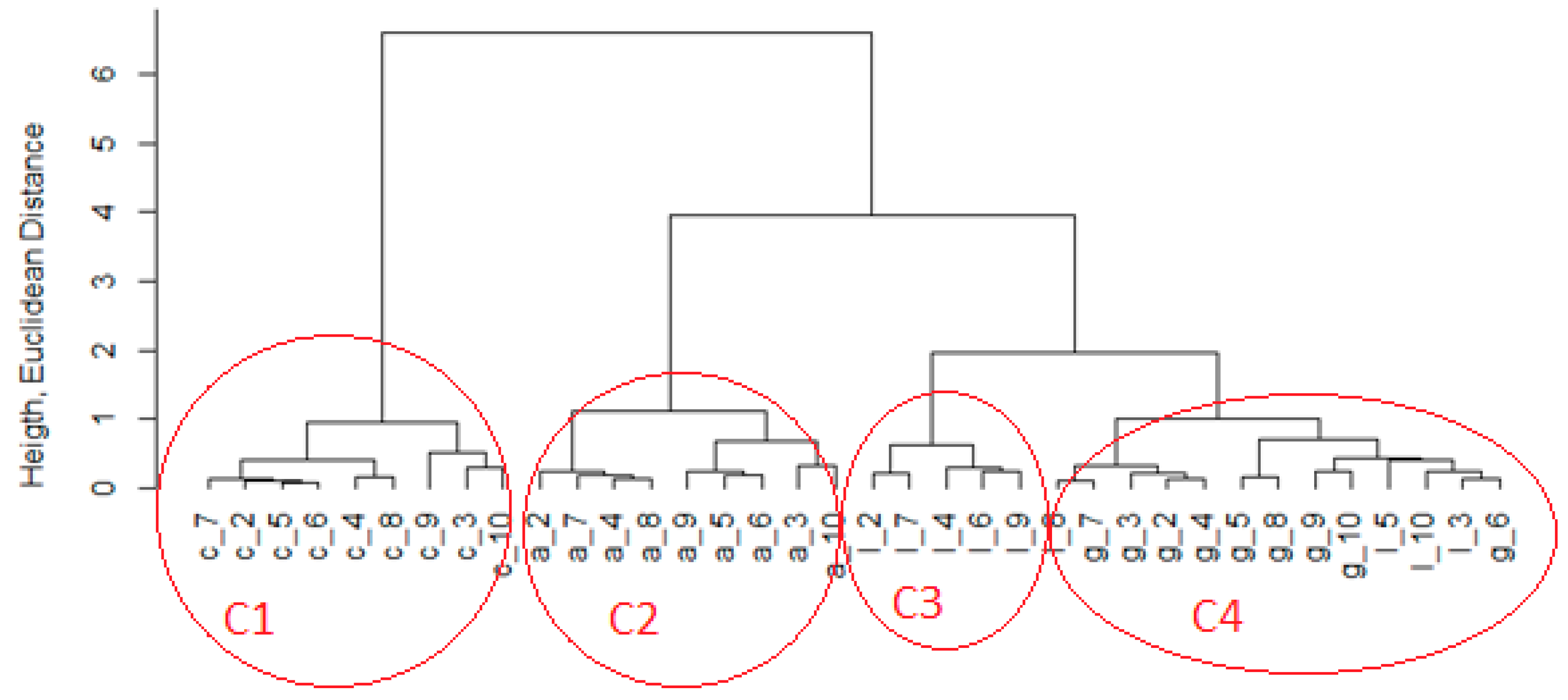
In the first step of the classification task, the Cluster dendrogram tool was used to determine the signal attributes for classification and determine the record length for calculating the attributes. The horizontal axis represents objects and clusters. The vertical axes on the dendrogram show the distance of the clusters, i.e., their dissimilarity. Each split of the two clusters is shown on the diagram by dividing the vertical line into two vertical lines. The position of the split, shown by a short line, indicates the distance (dissimilarity) between the two clusters.
From the original record, objects defined by a vector of vibration signal attributes were created for each type of material.
The goal was to find such attributes of the vibration signal and such length of the vibration signal for which there are as many objects of the same material as possible in each cluster, preferably all objects of the same material.
The One way ANOVA statistical test was used to search for suitable signal attributes for individual vibration signal parameters and lengths of vibration signal [
20]. The sorting factor was the material type. Assumptions for the use of ANOVA are: the population of residuals must be close to a normal distribution (the Shapiro-Wilk test was used to verify this condition [
21], (the population variances must be equal (i.e., homoscedastic), It was used Bartlett test of homoscedasticity [
22].
The TUKEY pairwise test is used for pair comparison of attributes between groups formed by individual materials. The decision criterion is the value of
p_
adj, which is compared with the level of significance, as well as the value of
p-value [
23].
In the second step of the classification task, the determination of the classification rule was left to the algorithm of the machine learning tool, the decision tree classifier [
24].
A decision tree for classification tasks works as follows: each internal node is labeled with an input feature. The leaves coming from the node marked by the input character are marked with each of the possible values of the destination character, or the leaf leads to a child decision node on the next input character. Each leaf of the tree is labeled with a class or a probability of distribution within the classes [
25]. At AdaBoost process, is the principle of boosting algorithms that we first build a model on the training data set and then build a second model to correct the errors present in the first model. This procedure continues until and unless the errors are minimized, and the data set is correctly predicted. Boosting algorithms work in a similar way, combining multiple models (weak learners) to produce a final output (strong learners) [
26].
The objects consisting of vectors and attributes of the vibration signal of the material were randomly divided into train set and test set in the ratio of 80 % and 20 % of the whole [
27]. The train set was used to create a classification rule using a decision tree classifier. In the test set, a classification rule was used and subsequently, the reliability of the classification was verified - using a classification table in which the numbers of correct/incorrectly classified objects are recorded.
According to the following equation (1), the reliability of the classification was calculated. The value is given in (%).
Reliability of classification = count of right classified objects/ count of objects.
(1)
3. Calculation
This section describes the procedure for solving both parts of the classification task. At each step, partial results are presented, and the next step is determined.
Step 1: Selection for signal attributes for classification and estimate record length to calculate attributes.
There were 16384 values for each type of rock.
To obtain information about the nature of the data, time series were created from the data from ranked values, and the following attributes were calculated for them (
Table 2):
where
j is the order of the start point time series sequence,
l is the length of the time series sequence, the number of points of the time series.
Fluctuation - fluctuation through zero, is the number, how many times the sign of the vibration signal changes in the time series.
Count_peaks_10 is count of number of that points of time series, which absolute value of vibration signal is higher than 10 mm.s-2
Count_peaks_15 is count of number of that points of time series, which absolute value of vibration signal is higher than 15 mm.s-2
Count_peaks_20 is count of number of that points of time series, which absolute value of vibration signal is higher than 20 mm.s-2
Variab is var of time series (mm.s-2)2
Skew is skewness of time series; it is a coefficient, so it has no units.
Kurt is kurtosis time series; it is a coefficient, so it has no units.
Step 2: Evaluate of attributes' suitability
This section describes how the attributes, and the length of the signal sequence were selected for the purposes of classification.
Sequences with a length of 500 values were created from the vibration signal recording for each rock. Thus, 32 objects from each rock were created.
Table 2 shows the attributes of the first 3 objects for each rock. The Start order value is the sequence number of the first point of the vibration signal of the rock for which the attributes of the object's vibration signal have been calculated. Each row of
Table 2 is a vector of object. The object label consists of the first letter of the material name and the object's serial number.
In
Table 2, for the first object from each rock, the attributes of the signal Fluctuation, and Count_peaks have higher values than for other objects of the same material. This fact results from the procedure for recording a vibration signal, immediately after starting drilling. The drilling tool has touched the surface and the initial vibrations that have been recorded have high indicator values and do not match the values of the indicators from the recording at the time when the drilling tool was already in a working position inside the material. Such objects cannot be included in the analysis. Objects for which the Start_order is larger than 500 will be included in the analysis. This corresponds to a rise time of 1/36th of a second.
For randomly selected 10 objects from each material and attribute vector (
Sum_of_abs, Sum_o, Fluctuation, Count peaks_10, Count peaks_15, Count peaks_20, Variab, Skew, Kurt), we created a dendrogram (
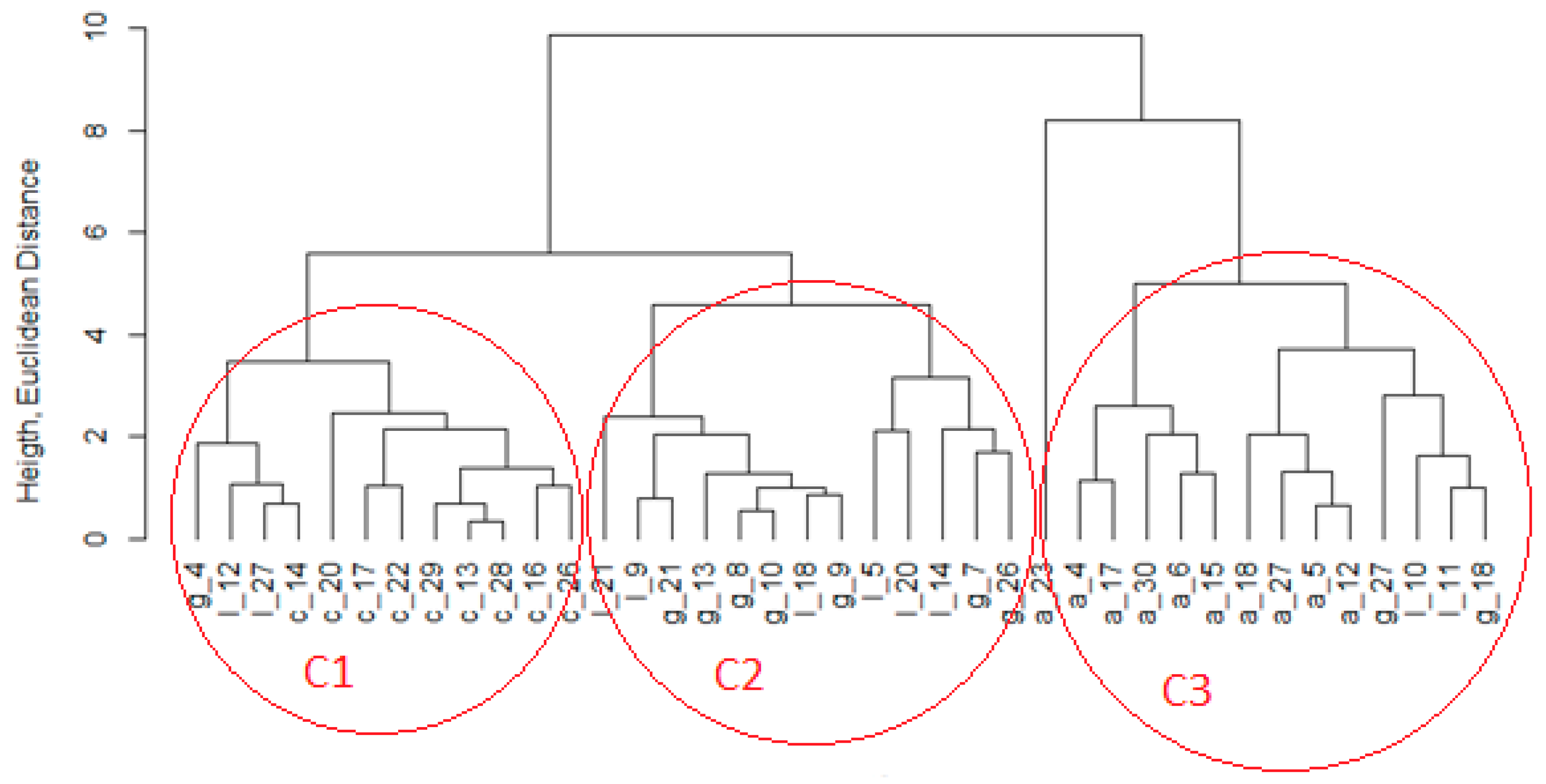
Figure 1) to verify that Euclid's distance from objects is less for objects of the same material than for objects of different materials from each other.
In the dendrogram (
Figure 1) we see that the classification into clusters is as follows:
Concrete objects - C are situated in one cluster of the second level C1; with them, there are two more objects of limestone - l and one object of granite - g. The first level cluster on the right C3 acts compactly, in which all andesite objects are located. However, there are also 2 objects limestone - l, and 2 objects granite - g. The cluster of the second level in the center of dendrogram C2 contains objects limestone - l, and granite - g.
The efficiency of sorting by dendrogram is 48 %. If we tried to classify arcs using such vibration signal attributes for sequences with a length of 500 values, 19 objects out of 40 would be correctly classified.
For the selected vibration signal attributes, using the ANOVA test (one-factor ANOVA, the factor is the type of material) and required related tests (Shapiro-Wilk test, Bartlett test), we verified which attributes are applicable to distinguish between rocks and which attributes, if they are part of objects, cause only noise and impair the possibility of distinguishing between materials (
Table 3).
To be suitable for distinguishing between materials, an attribute should have the following properties:
Rejected null hypothesis for ANOVA;
Conditions fulfilled distribution normality for residues - Shapiro-Wilk test;
Fulfilled conditions for homoscedasticity, the not rejected null hypothesis for Bartlett's test;
All TUKEY pairwise p_adj value less than 0.05.
Only Count Peaks_10 meets all the criteria (
Table 3).
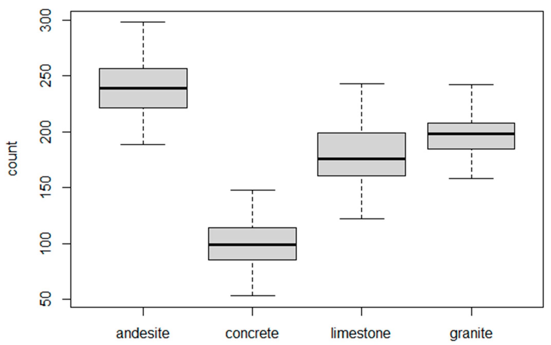
The box chart (
Figure 2) shows that the attribute values overlap for individual materials – material cannot be classified using this indicator alone.
The evaluation of findings: The vibration signal attributes used for the specified vibration signal length do not meet the purpose of classification. In addition to the differences in the values of the indicators for a vibration signal time series of 1500 values, there are also differences in the variability of some of the indicators. For this reason, we created new objects, this time from vibration signal attributes with a length of 1500 values. This corresponds to a recording length of 1/12th of a second.
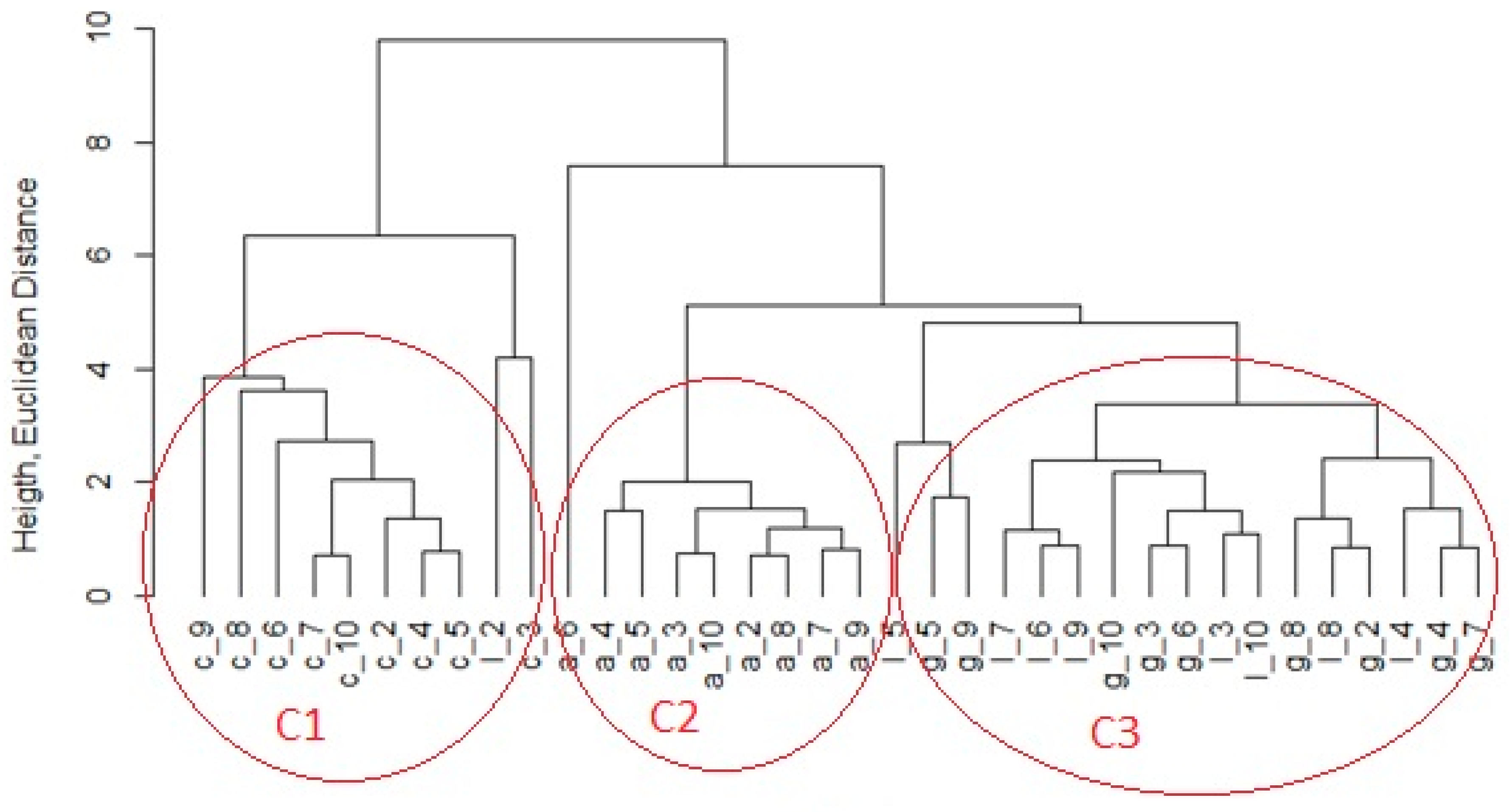
For the new sequence length of 1500 values, the classification into clusters has been improved, as can be seen in
Figure 3. We can conclude that the Euclidean distance between individual concrete objects - c, cluster C1 is smaller than between objects of concrete and other materials. The Euclidean distance between objects of granite - g and limestone -l is as small as between individual objects of limestone – l, and individual objects of granite – g (cluster C3).
To further improve, we decided to leave those attributes that are relevant to objects for sorting. The aim is to demonstrate their statistically significant influence on the classification of the object to the correct material and to exclude those attributes that cause noise when calculating Euclidean distance. For the selection of appropriate criteria, the same criteria were established for objects created from sequences of length 500 values.
The following
Table 4 presents calculated criteria values for objects created from sequences of 1500 values.
Where the criterion that the null hypothesis was not rejected for the ANOVA test was not met, the other criteria were not calculated.
Established criteria, they meet the indicators: Sum_of_abs, Count Peaks_10, Count Peaks_15, Variab. In addition to these, the Fluctuation attribute has been retained in the object vector.
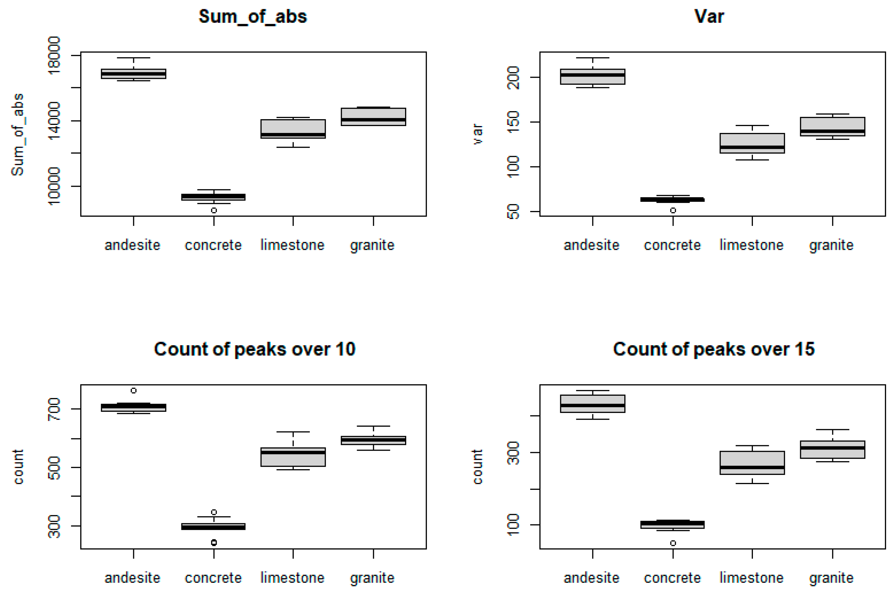
The following group of graphs (
Figure 4) displays a box plot for objects, sequences of 1500 values for each selected attribute.
It is clear from the graphs that distinguishing between concrete and andesite materials is easy. However, for the correct distinction between granite and limestone, this is insufficient. On the other hand, it is possible that using all the selected attributes, it will be possible to classify the objects of individual rocks correctly.
Cluster dendrogram (
Figure 5) is created from objects of individual materials, for 5 attributes. It has unambiguously Euclidean distances separated into clusters objects concrete - c in cluster C1, and andesite - a, and in cluster C2. The group of limestone objects - l is also classified into a single cluster, C3. The worst looks right cluster of the third level - C4, in which there are objects of granite - g, and objects of limestone - l.
Evaluation of findings: The vibration signal attributes used for a specified sequence length are not suitable for the purpose of classification.
The following procedure is chosen based on: Looking at the dendrogram (
Figure 5), and examining the classification of objects into clusters, it becomes clear that: Cluster C3 grouping limestone objects - l, contains at least one of three consecutive objects. That is, from objects l_2, l_3, l_4 contains objects l_2 and l_4; of objects l_3, l_4, l_5 contains object l_4; of objects l_4, l_5, l_6 contains l_4 and l_6; Objects l_5, l_6 l_7 contains objects l_6 and l_7, objects l_6, l_7, l_8 contains l_6 and l_7; of objects l_7, l_8, l_9 contains l_7 and l_9; Of the objects l_8, l_9, l_10 contains l_9
.
Based on this finding, we create each object of material from three consecutive sequences of vibration signal with a length of 1500 values as follows: For each attribute, the object's attribute value will be the minimum of these three values. The total length of the sequence required to create each object will be 4500 values, this is 1/4 second. The objects created in this way will be used to determine the classification algorithm.
Further calculations are not necessary, as it is clear from the foregoing consideration that all objects of the same material will be included in the same cluster.
4. Results and Discussion
The classification of each rock was carried out separately in such a way: each object of rock was assigned a class attribute. If the object was created from the vibration signal of the classified material, the class value was 1; if it was created from the vibrational of other materials, the value of the class attribute was 0.
For classification purposes, objects were created from the vibration signal of rock in such a way that 4 x 100 random Start order values from the interval of minimum 501 and maximum 11884 were generated by a generator of worthy numbers. Random orders were randomly assigned to rocks. 100 objects were created for each material, making a total of 400 objects.
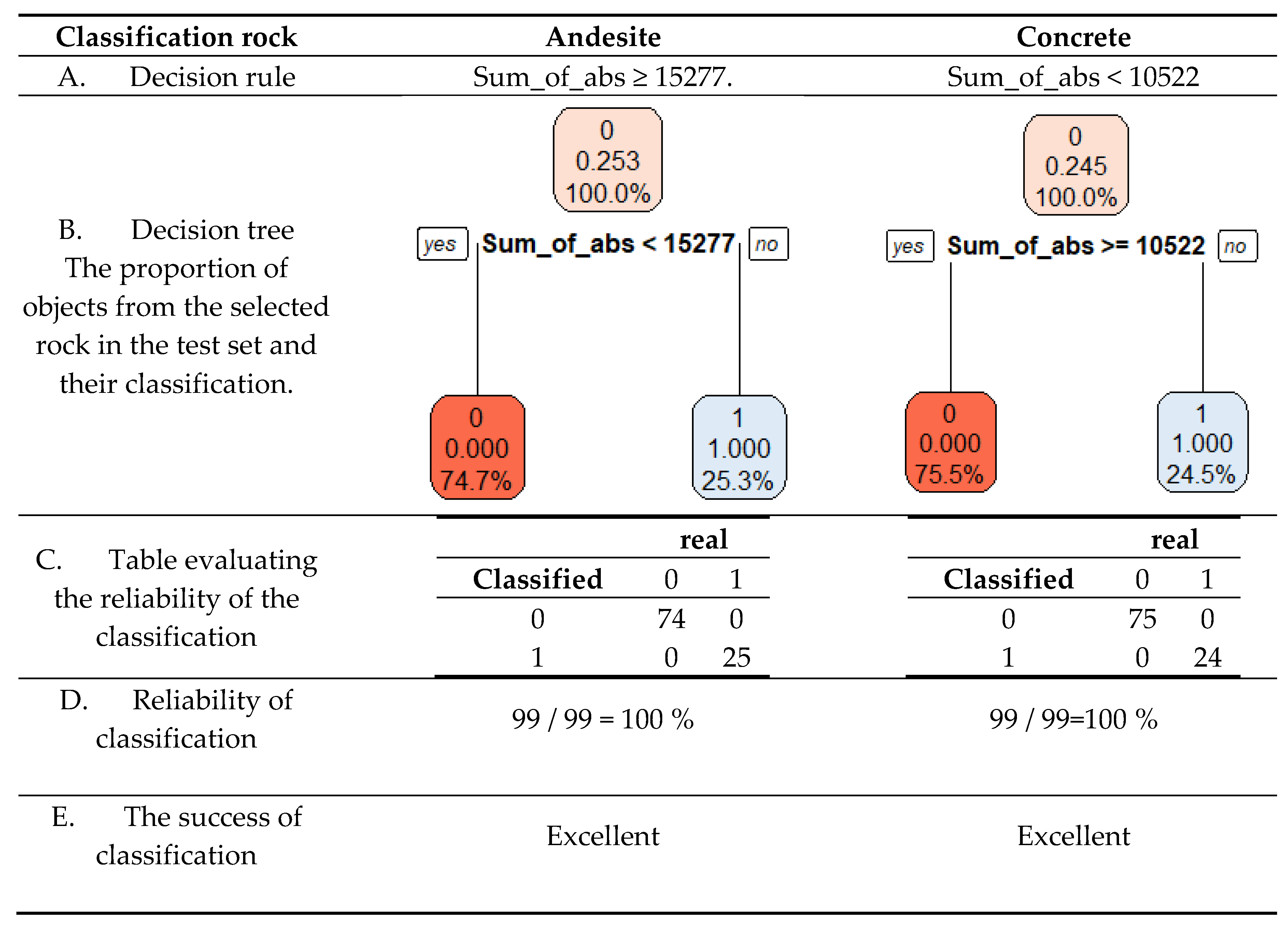
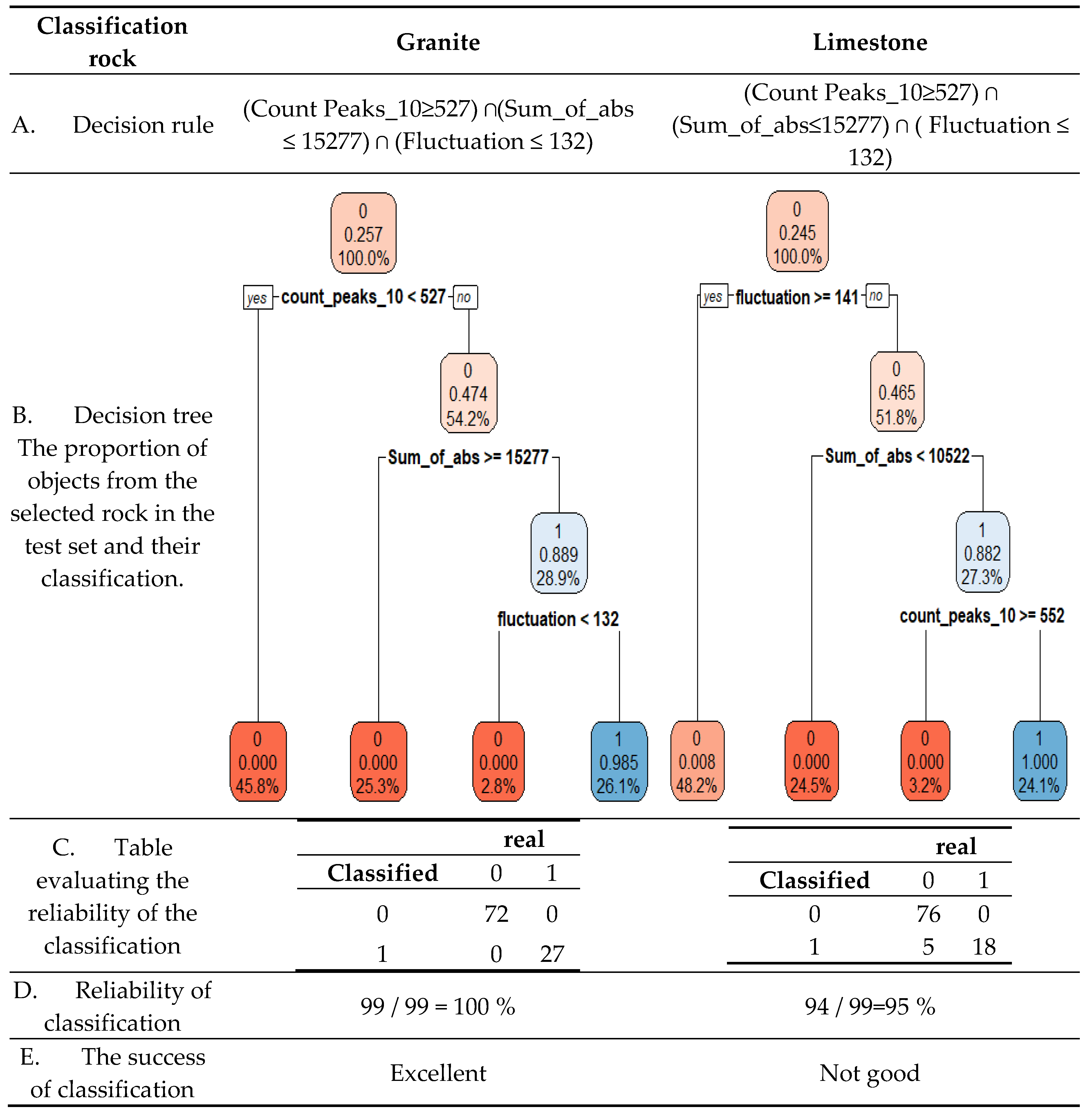
The classification was then implemented by a tool from the field of machine learning: a decision tree. In the next section, for each rock, we indicate (
Table 5,
Table 6):
- A.
Classification rule;
- B.
Decision tree for train set;
- C.
Table evaluating the reliability of the classification;
- D.
A percentual expression of the reliability of classification;
- E.
Verbal evaluation of the success of classification.
To improve the classification rule, we used the AdaBoost method, based on the modified rule, the number, and location of incorrectly classified objects changed, but the reliability increased by only 1%, to 96%. This can be seen in
Table 6.
For the classification to be excellent, we propose the following procedure: In the case of the classification of 4 types of rocks, for the correct classification of the rock limestone, it is to gradually exclude 3 materials using their sorting criterion, while the reliability of the classification should remain 100 %.
5. Conclusions
The publication presents the process of proposing a rock classification method using the vibration signal of the rotary drilling process. This research follows the efforts of the authors [
28] to classify the rock based on a vibration signal from 2014 - when a cumulative periodogram was used as a classification method.
As a result, the relevant vibration signal attributes and their cut-off values for classification rules were determined for classifications in four rocks.
The data were randomly divided into a train set and a test set, with 80% and 20% respectively. The classification rules were also created from train set data using the decision tree machine learning tool. For the design of a suitable classification method, were calculated several attributes of vibration signal and to determine useful attributes and proper signal length was used cluster dendrogram, ANOVA test, and boxplot. The reliability of the classification of four rocks, andesite, granite, limestone, and concrete via this method is 100%.
The vibration signal was obtained from the experimental process of rotary drilling.
The method of rock classification using a vibration signal in the process of rotary drilling is prospective, with the recording time required for the classification of the material in the length of 1/4 s. For the method to be generalized, additional extracts would need to be implemented for a higher number of materials and multiple drilling modes.
Methods for estimating the hardness of drilled rock based on analysis of vibration acoustic signal from rock drilling are known from the literature [
18].
In our case, materials with similar hardness were not confirmed to have similar vibration signal attributes for the uniform sequences used.
The vibration signal of different rocks under the same drilling mode is influenced by multiple material attributes. There is a relationship between the attributes of the vibration signal and the attributes of the rock, such as the granularity and mineralogical composition, density, hardness, and others.
Rapid classification of drilled material can be useful, especially in deep drilling processes for process.
Author Contributions
Conceptualization, B.S., and G.B.; methodology, B.S., and G.B.; software, B.S.; validation, P.F; formal analysis, G.B. and B.S.; investigation, B.S., G.B., P.F., R.F. and L.D.; resources, B.S., G.B. and P.F.; data curation B.S. and P.F; writing—original draft preparation, B.S., G.B. and R.F.; writing—review and editing, G.B. and B.S.; visualization, B.S. and G.B.. All authors have read and agreed to the published version of the manuscript.
Funding
This research was funded by Slovak Grant Agency for Science under grant VEGA 1/0264/21.
Data Availability Statement
The data presented in the experiments may be available from the first author upon request.
Acknowledgments
This work was supported by the Slovak Grant Agency for Science under grant VEGA 1/0264/21 Application of modern methods in the analysis and modeling of technological and other processes used in the acquisition and processing of earth resources in order to optimize them.
Conflicts of Interest
The authors declare no conflict of interest.
References
- Chlebová, Z. Simulation Analysis of Vibratory Device Controlled Vibration. Acta Mech. Slovaca 12, 323–334.
- Krepelka, F.; Chlebová, Z.; Ivaničová, L. Measurement, Analyzes and Evaluation of Stochastic Processes Operating in Rock Drilling. Acta Mech. Slovaca 20, 229–236.
- Leššo, I.; Flegner, P.; Špak, E. Research of the Possibility of Application of Vector Quantisation Method for Effective Process Control of Rocks Disintegration by Rotary Drilling. Metalurgija 49, 61–65.
- Cirimello, P.; Otegui, J.L.; Martinez Sanchez, J.; Carfi, G. Oil Well Drill Bit Failure during Pull out: Redesign to Reduce Its Consequences. Eng. Fail. Anal. 2018, 83, 75–87. [Google Scholar] [CrossRef]
- Klaic, M.; Murat, Z.; Staroveski, T.; Brezak, D. Tool Wear Monitoring in Rock Drilling Applications Using Vibration Signals. Wear 2018, 408–409, 222–227. [Google Scholar] [CrossRef]
- Krepelka, F.; Chlebová, Z. Frequency Analysis of the Device Acoustical Response by Rock Drilling in Connection with Drilling Process Optimization. Acta Mech. Slovaca 11, 111–120.
- Rostami, J.; Kahraman, S.; Naeimipour, A.; Collins, C. Rock Characterization While Drilling and Application of Roof Bolter Drilling Data for Evaluation of Ground Conditions. J. Rock Mech. Geotech. Eng. 2015, 7, 273–281. [Google Scholar] [CrossRef]
- Gradl, C.; Eustes, A.W.; Thonhauser, G. An Analysis of Noise Characteristics of Drill Bits. OnePetro. 21 September 2008. [Google Scholar]
- Khoshouei, M.; Bagherpour, R.; Jalalian, M.H. Rock Type Identification Using Analysis of the Acoustic Signal Frequency Contents Propagated While Drilling Operation. Geotech. Geol. Eng. 2022, 40, 1237–1250. [Google Scholar] [CrossRef]
- Miklúšová, V.; Ušalová, Ľ.; Ivaničová, L.; Krepelka, F. Acoustic Signal – New Feature in Monitoring of Rock Disintegration Process. Contrib. Geophys. Geod. 2006, 36, 125–133. [Google Scholar]
- Qin, M.; Wang, K.; Pan, K.; Sun, T.; Liu, Z. Analysis of Signal Characteristics from Rock Drilling Based on Vibration and Acoustic Sensor Approaches. Appl. Acoust. 2018, 140, 275–282. [Google Scholar] [CrossRef]
- Yan, R.; Gao, R.X. Hilbert–Huang Transform-Based Vibration Signal Analysis for Machine Health Monitoring. IEEE Trans. Instrum. Meas. 2006, 55, 2320–2329. [Google Scholar] [CrossRef]
- Yang, J.-H.; Yao, C.; Lu, W.; Jiang, Q.; Jiang, S.-H.; Zhou, C. Vibration Frequency Characteristics of Surrounding Rock of Deep Tunnel Induced by Borehole-Blasting. Yantu LixueRock Soil Mech. 2017, 38, 1195–1202. [Google Scholar] [CrossRef]
- Flegner, P.; Kačur, J.; Durdán, M.; Laciak, M. Evaluation of the Acceleration Vibration Signal for Aggregates of the Horizontal Drilling Stand. Appl. Sci. 2022, 12, 3984. [Google Scholar] [CrossRef]
- Waloski, R.; Korzeniowski, W.; Bołoz, Ł.; Rączka, W. Identification of Rock Mass Critical Discontinuities While Borehole Drilling. Energies 2021, 14, 2748. [Google Scholar] [CrossRef]
- Kumar, B.R.; Vardhan, H.; Govindaraj, M. Sound Level Produced during Rock Drilling Vis-à-Vis Rock Properties. Eng. Geol. 2011, 123, 333–337. [Google Scholar] [CrossRef]
- Jiang, R.; Dai, F.; Liu, Y.; Li, A. A Novel Method for Automatic Identification of Rock Fracture Signals in Microseismic Monitoring. Measurement 2021, 175, 109129. [Google Scholar] [CrossRef]
- Wang, H.; Lu, S.; Huang, M.; Zhao, X. Hardness Identification of Rock Based on Multi-Sensor Information Fusion during the Process of Roadway Tunnelling. Bull. Pol. Acad. Sci. Tech. Sci. 2020, 1301–1309. [Google Scholar]
- Types of Rocks | Kinds of Rocks | Famous Rocks | Compare Rocks. Available online: https://rocks.comparenature.com/rocks.comparenature.com/ (accessed on 20 June 2023).
- Fisher, R.A. The Design of Experiments; The design of experiments; Oliver & Boyd: Oxford, England, 1935; pp. xi, 251. [Google Scholar]
- Shapiro, S.S.; Wilk, M.B. An Analysis of Variance Test for Normality (Complete Samples).
- Bartlett, M.S. The Statistical Conception of Mental Factors. Br. J. Psychol. Gen. Sect. 1937, 28, 97–104. [Google Scholar] [CrossRef]
- Tukey, J.W. One Degree of Freedom for Non-Additivity. Biometrics 1949, 5, 232–242. [Google Scholar] [CrossRef]
- Therneau, T.; Atkinson, B.; Ripley, B. Rpart: Recursive Partitioning and Regression Trees Version 4.1.19 from CRAN. Available online: https://rdrr.io/cran/rpart/ (accessed on 21 June 2023).
- Milborrow, S. Rpart.Plot: Plot “rpart” Models: An Enhanced Version of “Plot.Rpart” 2022.
- Alfaro, E.; Gamez, M.; García, N. Adabag: An R Package for Classification with Boosting and Bagging. J. Stat. Softw. 2013, 54, 1–35. [Google Scholar] [CrossRef]
- Tuszynski, J. CaTools: Tools: Moving Window Statistics, GIF, Base64, ROC AUC, Etc 2021.
- Flegner, P.; Kačur, J.; Durdán, M.; Leššo, I.; Laciak, M. Measurement and Processing of Vibro-Acoustic Signal from the Process of Rock Disintegration by Rotary Drilling. Measurement 2014, 56, 178–193. [Google Scholar] [CrossRef]
|
Disclaimer/Publisher’s Note: The statements, opinions and data contained in all publications are solely those of the individual author(s) and contributor(s) and not of MDPI and/or the editor(s). MDPI and/or the editor(s) disclaim responsibility for any injury to people or property resulting from any ideas, methods, instructions or products referred to in the content. |
© 2023 by the authors. Licensee MDPI, Basel, Switzerland. This article is an open access article distributed under the terms and conditions of the Creative Commons Attribution (CC BY) license (http://creativecommons.org/licenses/by/4.0/).
