Preprint
Article

Predictive Modeling of Delay in an LTE Network by Optimizing the Number of Predictors Using Dimensionality Reduction Techniques

Altmetrics

Downloads

84

Views

21

Comments

0

A peer-reviewed article of this preprint also exists.

Submitted:

29 June 2023

Posted:

30 June 2023

You are already at the latest version

Alerts
Abstract
Delay in data transmission is one of key performance indicators (KPIs) of a network. The planning and project value of delay in network management is of crucial importance for the optimal allocation of network resources and their performance focuses. To create optimal solutions, predictive models, which are currently most often based on machine learning (ML), are used. This paper aims to investigate the training, testing and selection of the best predictive delay model for a VoIP service in an Long Term Evolution (LTE) network using three ML techniques - Neural Networks (NN), Support Vector Machines (SVM) and k-Nearest Neighbors (k-NN). The space of model input variables is optimized by dimensionality reduction techniques: RReliefF algorithm, Backward selection via the recursive feature elimination algorithm and the Pareto 80/20 rule. A three-segment road in the geo-space between the cities of Banja Luka (BL) and Doboj (Db) in the Republic of Srpska (RS), Bosnia and Herzegovina (BiH), covered by the cellular network (LTE) of the M:tel BL operator was chosen for the case study. The results show that, in all three optimization approaches, the k-NN model is selected as the best solution. For the RReliefF optimization algorithm, the best model has 6 inputs and minimum relative error (RE), RE=0.109; for the Backward selection via the recursive feature elimination algorithm, the best model has 4 inputs and RE=0.041; and for the Pareto 80/20 rule, the best model has 11 inputs and RE= 0.049. The comparative analysis of the results concludes that according to observed criteria for the selection of the final model, the best solution is an approach to optimizing the number of predictors based on the Backward selection via the recursive feature elimination algorithm.
Keywords: 
Subject: Engineering  -   Telecommunications

1. Introduction

Sustainable Quality of Service (QoS) for users is one of the main tasks of mobile operators. This orients them to provide comprehensive support for various applications and services with numerous QoS requirements in order to meet the expected levels of user Quality of Experience (QoE) [1,2]. The development of Long Term Evolution (LTE) technology, which today is based on IP network configuration [3], is an example of such an orientation. The target reason is optimal performance, i.e. low delay, high data transfer speed, as well as better optimization of packet transfer. In addition to the mentioned key features of LTE network technology, there is Radio Resource Management (RRM), which can raise network performance almost to the level of the Shannon limit [4]. An important operational technology of LTE is Packet scheduling for assigning to each User Equipment (UE) a part of network resources depending on QoS requirements, but also on the impact of delay, channel quality, number of active UEs, throughput, etc. During the congestion in the network, users’ QoS requirements increase, and today popular interactive real-time services, such as Voice over IP (VoIP), i.e. Voice over Long Term Evolution (VoLTE) and streaming, are the most sensitive and susceptible to degradation during that period. Key network performance indicators during congestion are end-to-end (E2E) delay and jitter, which represents variations in delay [5]. According to the standard 123 107 v12.0.0 (2014) of the European Telecommunications Standards Institute (ETSI) [6], the maximum tolerated delay for VoIP services is defined as 100 ms, and 300 ms for streaming services. End-to-end delay can be defined as the time required for a data packet to be transmitted through a network from a source node to a destination node, and in a VoIP network it consists of the sum of transmission delay, signal propagation delay and packet waiting delay.
Current research in various fields shows that predictive models, which predict events and situations from the present towards the future based on data from the past, have an enormously wide range of applications. Especially in telecommunications, predictive models are most often based on machine learning (ML) techniques. The actuality and application of predictive models using ML techniques are encouraged by a very rapid increase in the amount of multidimensional data - Big Data (BD) publicly available on the Internet. BD increases the complexity of the problem of finding the optimal way to the solution to functional tasks in the network domain. At the same time, the high dimensionality of data, i.e. a large number of variables often makes it difficult to create a model and jeopardizes the accuracy of prediction results. Among the discovered approaches to solutions for reducing the problem of complexity, as a key indicator of the state configuration in the situational dynamics of telecommunication traffic, data preprocessing by dimensionality reduction techniques is used. Data dimensionality reduction implies optimization of the space of input/independent variables and the number of predictors, but with the obligation to preserve relevance and other qualitative attributes of information [7]. Feature Selection is one of the most common and important dimensionality reduction techniques, and, in research papers, it is also known as variable selection, attribute selection or variable subset selection. In this paper, the research focus is on three dimensionality reduction approaches: RReliefF algorithm, Backward selection via the recursive feature elimination algorithm and the Pareto 80/20 rule, where the first two approaches belong to Feature selection techniques. The selection of input variables is a process that includes the detection of variables that have a significant impact on the prediction of output, and the removal of redundant variables. As the main benefits achieved by this technique, the following can be highlighted: increasing the speed of data mining algorithms, increasing the accuracy of prediction, reducing the complexity of the model [7,8].
Starting from the assumption that better planning and design of networks and allocation of network resources can be achieved in the future if the value of end-to-end delay is known, this paper examines the performance of three predictive delay models for a VoIP service in an LTE network based on Neural Networks techniques (NN), Support Vector Machines (SVM) and k-Nearest Neighbors (k-NN), whose input set of variables is optimized [9]. As a case study, the geographic area in the Republic of Srpska (RS), Bosnia and Herzegovina (BiH), in the vicinity of a three-segment road between the cities of Banja Luka (BL) and Doboj (Db), which is covered by the cellular network of the M:tel BL operator, is chosen. The main goal is to select an ML model with an optimal number of input variables, which provides the most accurate prediction results.
The most important aims and objectives of this research are the following:
  • Reducing the dimensionality of the space of model input variables by optimization with Feature Selection techniques (RReliefF and Backward selection via the recursive feature elimination algorithms) and the Pareto 80/20 rule;
  • Training and testing of ML models: NN, SVM and k-NN with the selection of the best delay prediction model in the LTE network using accuracy and complexity/interpretability criteria;
  • Presentation of the aforementioned approaches to optimizing the number of predictors for LTE KPI predictive modeling, which is, according to the authors' knowledge and according to the review of former research papers, a particularly innovative solution given in this paper;
  • Implementation of a unique methodology of indirect assessment and calculation of the value of the dependent variable based on the average number of active users in the network;
  • Creation of universally applicable predictive modeling of delays in the LTE network based on real research, and a data space connected to one of the most important roads in the geo-road network of RS, BiH, was chosen for the case study.
The paper is structurally divided into five sections. After the introductory part, Section 2 presents a review of relevant published research papers, and Section 3 contains the materials and methods used in the paper. The main research focus is on Section 4 where the results and discussion are provided, after which the conclusions are drawn in Section 6. The references used are listed in the last section of the paper, after the conclusion.

2. Review of Relevant Published Research

In the research [10], the authors created models for end-to-end delay prediction in Cellular Vehicle-to-Everything (C-V2X) communication using different ML techniques. Model training was performed on KPI-related variables, and data was collected from real LTE networks. In this paper, prediction is viewed as a delay classification problem depending on a given threshold. Similar research is conducted in [11] with a focus on delay prediction for V2X applications in Mobile Cloud/Edge Computing systems. The proposed prediction framework in this case consists of a component based on machine learning techniques and a statistical component. The paper [12] presents an algorithm for resource allocation prediction in LTE uplink (UL) connection for machine to machine (M2M) applications. Mathematical models for prediction probability, successful prediction probability, failed prediction probability, resource utilization/underutilization probability, and mean uplink delay model were developed. All these models are validated using a simulation model implemented on the OPNET platform. An original approach based on machine learning for delay prediction in 4G networks is presented in [13]. To create the model, the authors use real data from three different mobile networks. The paper [14] considers a case study related to the Industrial Internet of Things (IIoT) in which the potential of digitization of mines is investigated. For this purpose, a software tool for sending sensor data using the LTE network is presented, and predictive delay models are created in order to evaluate the network performance. Lai & Tang (2013), in their paper [15], develop a Packet Prediction Mechanism (PPM), based on mathematical models, for delay prediction when using real-time services. The main research focus is on a virtual queue concept, which has the function of predicting the behavior of incoming packets in the future based on the packets currently in the queue. Due to the increasing user demand for real-time services, the development of wireless access technologies that provide greater bandwidth is evident every day. Therefore, the same team of authors, in the published research paper [16], proposes and designs LTE scheduling mechanism and PPM. In doing so, the authors assume that the proposed PPM will increase capacity, reduce resource consumption and thereby increase network efficiency. Starting from the assumption that the monitoring and prediction of QoS indicators are the basic prerequisites for user satisfaction in the use of LTE network services, delay and average user throughput are considered as key indicators of network performance in the paper [17]. The authors have created models to estimate the values of these dependent variables as linear functions of total network traffic and average Channel Quality Indicator (CQI). In [18], the subject of research is the changes in Round-trip time (RTT) delay and the prediction of the increase in these values in mobile broadband networks. Four classification models based on machine learning were developed, using data from a large number of probes in the network, and the best classification performance was shown by the binary ensemble model.
The essential characteristics of the previously analyzed papers are shown in Table 1. For each paper marked with a reference number, the models and techniques used, the prediction problem being solved (regression/classification), the service/application being observed, and some of the dimensionality reduction methods and techniques if applied are given.
Compared to previously analyzed published research papers, the following five contributions stand out as the main improvements and novelties presented in this paper:
  • Network delay is investigated by observing a real geospatial and LTE network segment as very important factors affecting KPIs;
  • The number of predictors in LTE delay examination is optimized for the first time simultaneously using three approaches for predictive modeling of delays in the LTE network;
  • A complete set of 17 independent/input research variables is used and Dimensionality Reduction is explained in detail;
  • The original indirect method of assessment and calculation of the values of the dependent/output variable is applied;
  • The optimization of the set of input variables is modeled with Feature Selection techniques and the Pareto 80/20 rule, and the obtained results are compared according to the criteria of prediction accuracy and complexity/interpretability of the model.

3. Materials and Methods

The research process in this paper was completed through several successive steps:
  • Analysis of a real geospatial and network research segment in the case study;
  • Data collection and analysis of independent research variables;
  • Calculation of dependent variable values;
  • Structuring data into input/output vectors;
  • Optimization of a set of independent variables by Feature Selection techniques: RReliefF and Backward selection via the recursive feature elimination algorithms;
  • Optimization of a set of independent variables by the Pareto 80/20 rule;
  • Training and testing of predictive delay models over an optimized set of independent variables;
  • Comparative analysis of prediction results and selection of the final model.

3.1. Geospatial and network research segment – a case study

For the case study in this paper, a three-segment road connected by a geodesic line, in the geo-space of RS, BiH, between the cities of BL and Db, consisting of the following road segments, was chosen:
  • A segment of the Motorway 9th January (M9J), 72 km long, between the Jakupovci toll station, near the city of BL, and the Kladari toll station, near the town of Db;
  • A segment of the M16 Main Road, about 6 km long, on the route Jakupovci – entrance to the city of BL;
  • A segment of the M17 trunk road, about 10 km long, located between the Kladari toll station and the town of Db.
In the observed geo-space, the research focus is on the fourth generation (4G) telecommunications network based on LTE network technology, managed by the M:tel BL provider [1,2]. Figure 1 shows a part of the geographical map (Google Earth) of the RS and BiH with marked areas of road segments, where the area marked in blue is covered by LTE Carrier Aggregation (CA), and the area in green is covered by LTE Frequency Division Duplexing (FDD) technology.
LTE CA is one of the key technologies used to achieve very high data transfer speeds in 4G networks. The principle is based on combining more than one signal carrier (in the same or different bands), to increase the bandwidth and channel capacity. In the observed case study, out of the total geographical area, 14.75% is covered by LTE CA technology, and 85.25% by LTE FDD technology, which enables duplex communication between eNB and UE and is based on paired spectrums with sufficient spacing between frequency domains to enable simultaneous sending and receiving of data.

3.2. Analysis of independent research variables and data collection

In this research, the following 17 independent variables or predictors selected from the set of research data provided by the M:tel operator are observed: 1) Cell; 2) Downlink (DL) PRB Usage Rate; 3) Average CQI; 4) DL ReTrans Rate; 5) UL ReTrans Rate; 6) DL IBLER; 7) UL IBLER; 8) Cell Traffic Volume DL; 9) Cell Traffic Volume UL; 10) Cell Downlink Average Throughput; 11) Cell Uplink Average Throughput; 12) Average DL User Throughput; 13) Average UL User Throughput; 14) UL Average Interference; 15) DL.QPSK.TB.Retrans; 16) DL.16QAM.TB.Retrans; 17) DL.64QAM.TB.Retrans.
The M:tel BL mobile operator provided the collected data for research purposes based on the official Request, which specified the necessary variables related to KPIs, radio channel properties, utilization of physical resources, number of users, eNodeB parameters, cell parameters, network topology and signal parameters in the observed research geo-space [19]. From the obtained database, for the purposes of this research, the values of the variables for the period of data collection between January 1, 2021 and January 15, 2021 and with a one-hour sampling frequency were extracted. After filtering missing and unusual values, a final database was formed consisting of a total of 31143 measurements structured in an Excel file, for each of the observed independent variables.
1) Cell
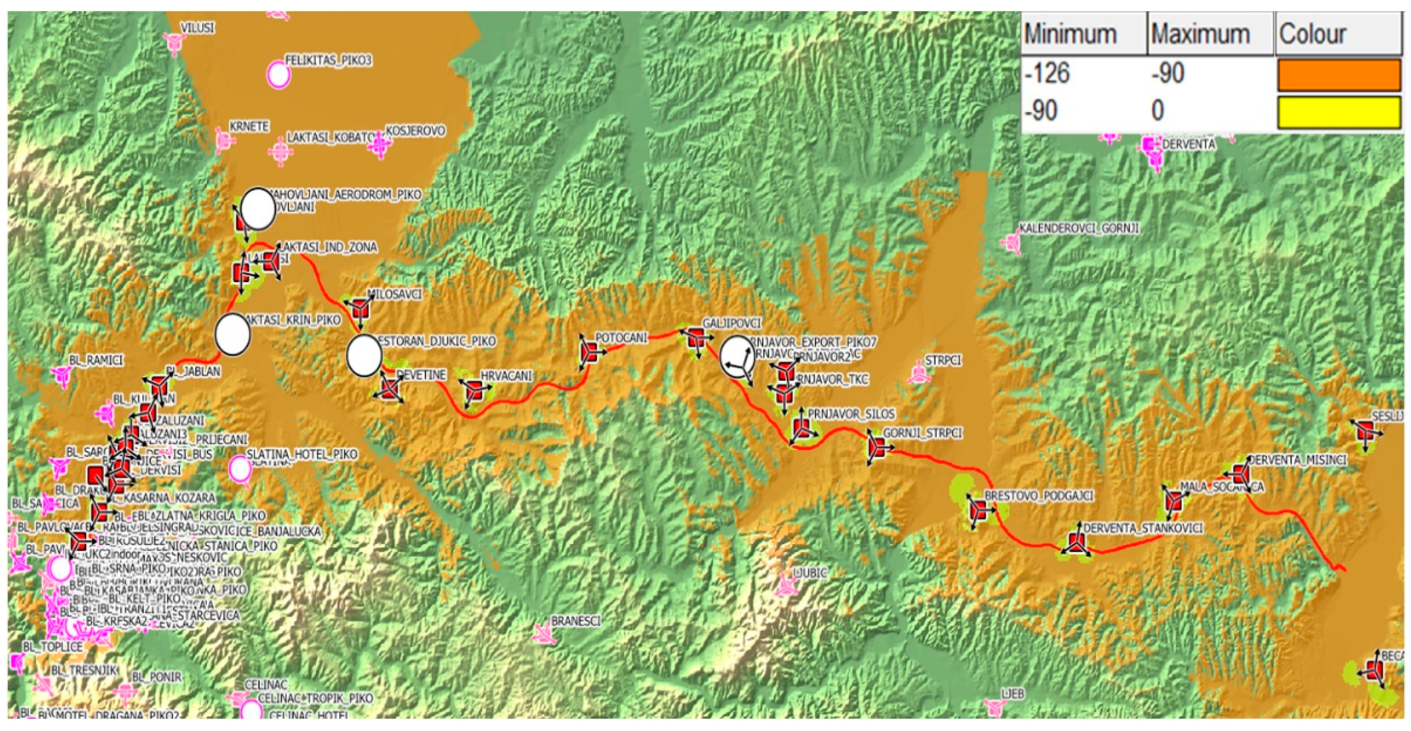
The access LTE network of the M:tel operator in the area of the observed three-segment road consists of a large number of eNodeBs that provide the connection of the UE with the rest of the 4G network. Their locations are represented by red squares in Figure 2. According to the number of mobile users, it is obvious that the highest density of eNodeB deployment is in the vicinity of BL city [19]. Also, in Figure 2, based on the colors, and according to the map legend, areas with different levels of signal attenuation can be identified, namely areas between -126 dB and -90 dB, and areas between -90 dB and 0 dB. Each of the eNodeBs covers one or more cells with a signal, and a total of 87 cells can be identified in the observed area.
2) DL PRB Usage Rate
In LTE networks, the smallest unit of radio resources that can be allocated to a user is a Physical Resource Block (PRB) consisting of 84 resource elements (7 symbols of 0.5 ms duration × 12 subs of 15 kHz each). When available but unused PRBs are not sufficient to serve all active users, it can cause the degradation of quality of service (QoS). DL PRB Usage Rate represents the ratio of the average number of used physical blocks in the Physical Downlink Shared Channel (PDSCH) and the total number of DL PRB available, multiplied by 100. PDSCH represents a DL physical shared channel whose priority function is the transmission of user data, but also the transmission of data essential for control, and DL system information [19].
3) Average CQI
The Channel Quality Indicator (CQI) can have a numerical value between 1 and 15, which the mobile device sends over the uplink connection to the eNodeB. Based on the received CQI value, the eNodeB selects the appropriate Modulation and Coding Scheme (MCS), thereby defining the data transmission rate in the communication channel. The Signal to Interference & Noise Ratio (SINR) and the characteristics of the mobile device determine the CQI value, such that the Block Error Rate (BLER) does not exceed 10%. This means that each CQI value is mapped to a specific MCS: Quadrature Phase Shift Keying (QPSK), Quadrature Amplitude Modulation (QAM, 16QAM, 64QAM). Each MCS corresponds to a specific Code Rate and number of bits per symbol [19,20].
4) DL ReTrans Rate & 5) UL ReTrans Rate
When the communication between the eNodeB and the user equipment is not established on the first or any subsequent attempt, data resending or retransmission is performed. Data is sent in packets, i.e. in a Transport Block (TB) within one Transmission Time Interval (TTI) with its duration of 1 ms. The DL/UL retransmission rate can be defined as the ratio of retransmitted packets (packets sent with retransmission) to all packets sent via the transport DL/UL SCH [19].
6) DL IBLER & 7) UL IBLER
Block Error Rate (BLER) is defined as the ratio between the total number of blocks transmitted in a message and the number of blocks in the same message received with an error. This ratio is a measure of the quality of a data transmission and is expressed as a percentage. On the receiving side of the telecommunications system, detection of such transmission errors is performed by the Cyclic Redundancy Check (CRC) technique. The Initial Block Error Rate (IBLER) is an indicator used to evaluate network performance and which shows the relationship between the number of blocks with initial transmission errors and the total number of initially transmitted TBs in the DL and UL direction [19].
8) Cell Traffic Volume DL & 9) Cell Traffic Volume UL
Cell Traffic Volume DL/UL represents the total aggregated DL/UL traffic in the cell in a period of one hour expressed in Gbit. In LTE networks, the total aggregated traffic represents the sum of traffic in 9 classes, which are identified by the QoS Class Identifier (QCI) [19]. The classes marked with QCI 1, QCI 2, QCI 3 and QCI 4 are characterized by a defined and guaranteed throughput of Guaranteed Bit Rate (GBR), and examples of services that belong to them are QCI 1 - Conversational Voice; QCI 2 – Conversational Video (Live Streaming); QCI 3 – Real Time Gaming; QCI 4 – Non-Conversational Video (Buffered Streaming). Non-GBR classes are marked with QCI 5, QCI 6, QCI 7, QCI 8, QCI 9 and imply a certain risk of packet loss, especially in conditions of network congestion. Examples of services belonging to them are QCI 5 – IMS Signalling; QCI 6 - Video (Buffered Streaming), TCP-based (www, e-mail, chat, ftp, p2p file sharing, progressive video, etc.); QCI 7 – Voice, Video (Live Streaming), Interactive Gaming; QCI 8 and QCI 9 - Video (Buffered Streaming), TCP-based (www, e-mail, chat, ftp, p2p file sharing, progressive video, etc.).
10) Cell Downlink Average Throughput & 11) Cell Uplink Average Throughput
One of the most important indicators of network performance is Throughput, which can be defined as the ratio of the amount of data transferred and the time for which the transfer is made. The variable Cell Downlink/Uplink Average Throughput represents the average value of this indicator for a period of one hour, at the level of one cell in the DL and UL direction. The average throughput value can be determined not only geographically (per spatial unit-cell), but also logically (per service) [19].
12) Average DL User Throughput & 13) Average UL User Throughput
The average value of Throughput at the user level in the LTE network, in the observed space in the DL and UL direction, is determined by the value of the Average DL/UL User Throughput variable. Also, this value is calculated for a period of one hour [19].
14) UL Average Interference
The total power of the noise floor and the interference of neighboring cells, received by each PRB, is measured during one TTI in the UL direction. The eNodeB divides the total power of the noise floor and the interference of neighboring cells by the number of PRBs, and the resulting value is used as the sampling result. At the end of the one-hour measurement period, the average of these sampling results expressed in dBm is used as the value of the UL Average Interference variable [21].
15) DL.QPSK.TB.Retrans, 16) DL.16QAM.TB.Retrans & 17) DL.64QAM.TB.Retrans
The variables DL.QPSK.TB.Retrans, DL.16QAM.TB.Retrans and DL.64QAM.TB.Retrans are related to the variable DL ReTrans Rate and refer to retransmission rates for certain modulation schemes. Their meaning is as follows:
  • 15) DL.QPSK.TB.Retrans - Number of retransmitted TBs in DL SCH at Quadrature Phase Shift Keying (QPSK) modulation;
  • 16) DL.16QAM.TB.Retrans - Number of retransmitted TBs in DL SCH at Quadrature Amplitude Modulation (QAM) with 16 carrier states (16QAM);
  • 17) DL.64QAM.TB.Retrans - Number of retransmitted TBs in DL SCH at QAM with 64 carrier states (64QAM).

3.3. Calculation of dependent variable values

End-to-end delay (DEtoE) consists of the sum of the delay at the Medium Access Control (MAC)/Radio Link Control (RLC) layer, which makes up the largest part of DEtoE, then of the delay due to signal propagation at the physical level and the transmission delay between the eNodeB and UE [22]. Therefore, the delay in this case implies "the time duration that starts when a flow is generated by a traffic source, transmitted through the communication system, until it reaches the application layer of the user's device - UE" [22].
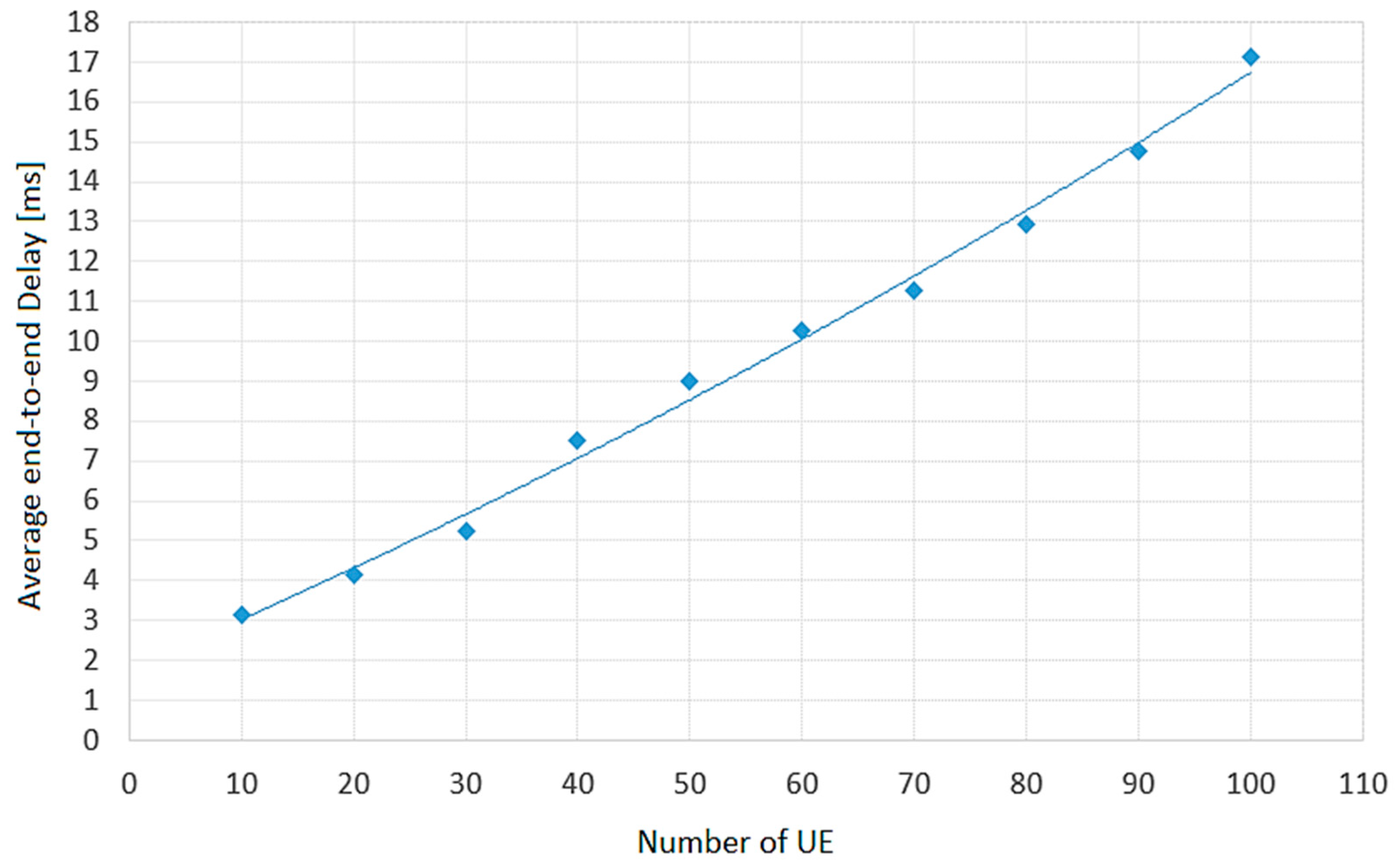
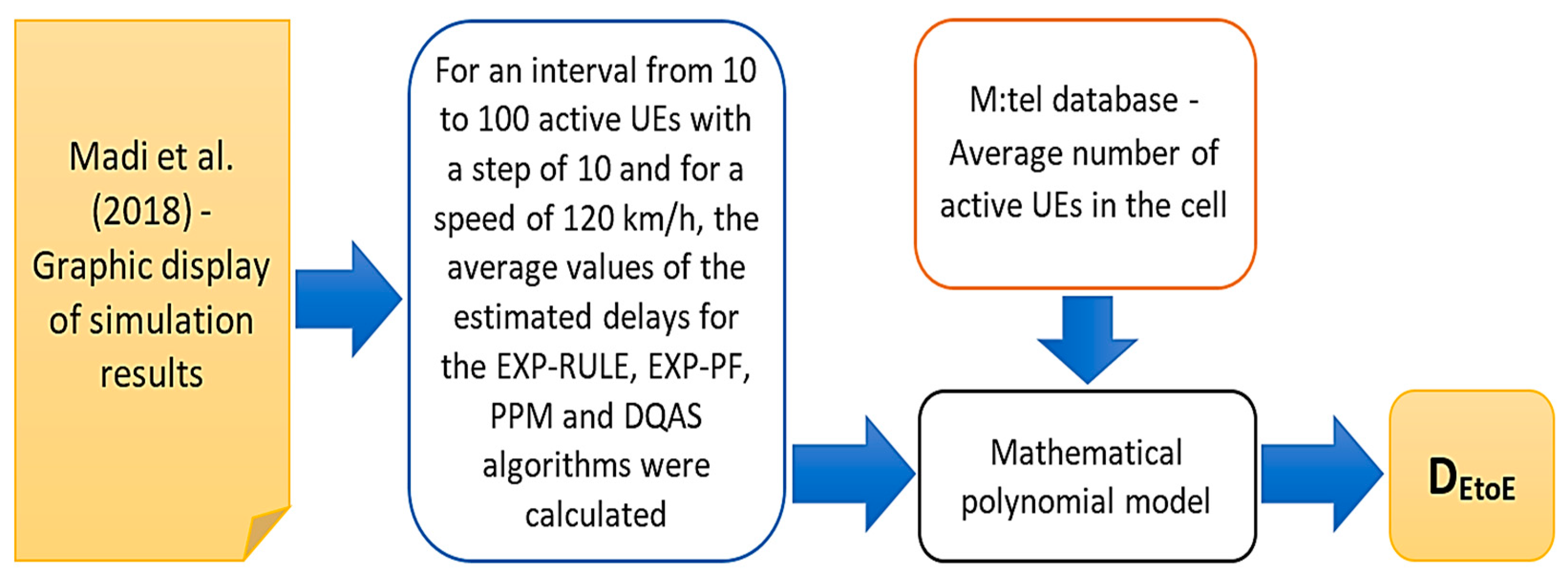
The values of the variable DEtoE were collected by estimation and calculation based on the results presented in the paper [22]. In this paper, Madi et al. (2018) used a simulation method to measure the end-to-end delay for VoIP traffic depending on the number of active UEs in the cell, at mobile user speeds of 3 km/h and 120 km/h for each of the four observed scheduling algorithms: Exponential Rule (EXP-RULE), Exponential-Proportional Fair (EXP-PF), PPM and Delay–based and QoS–Aware Scheduling (DQAS). Based on graphically presented simulation results in [22] (Fig. 7 Average DE2E on RT VoIP flows), for an interval from 10 to 100 active UEs in a cell with a step of 10 and for a speed of 120 km/h, average values of the estimated delays for the four observed scheduling algorithms are calculated in this paper. The values calculated in this way are shown by points in Figure 3, where the regression curve that best describes the functional dependence of the average delay on the number of UEs is given.
The curve shown in Figure 3 has a polynomial form of the second degree and can be represented by a quadratic equation as follows:
D e l a y = 0.0003 · U E 2 + 0.1197 · U E + 1.8071
As an indicator of the quality of this model, a very high coefficient of determination (R2), which is R2=0.9941, appears. Considering that the database obtained from the M:tel operator, among other things, provided the values of the average number of active UEs in the cells of the observed geographical area, the DEtoE values were obtained indirectly, by calculation based on the model given by Eq. (1), which is shown graphically in Figure 4.
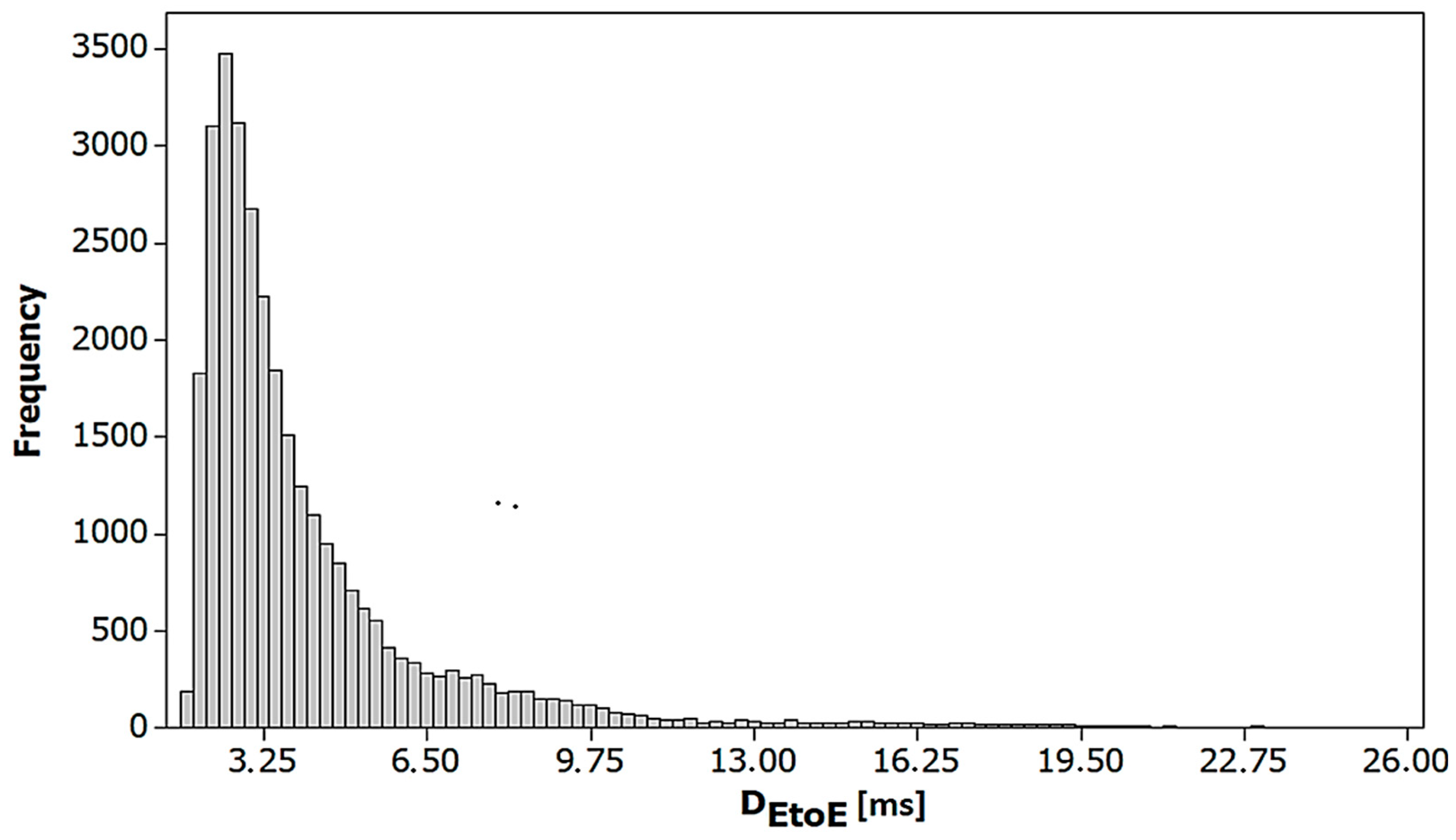
Descriptive statistics for the dependent variable are given in Table 2, and the histogram of the DEtoE variable is shown in Figure 5.
By a more detailed analysis of the histogram shown in Figure 5 (in Minitab software), it is concluded that DEtoE values in the range between 2.375 ms and 2.625 ms have the highest frequency of 3477 repetitions. The arithmetic mean of the delay values is 4.1503 ms, and of the median is 3.2516 ms.

3.4. Structuring data into input/output vectors

Considering that data processing in this research is performed by ML techniques, it is necessary to structure the values of independent variables and the values of the dependent variable into input/output vectors [9]. This kind of data structure enables the training of the ML model according to the supervised learning paradigm, where the independent variables have the role of inputs to the model, and the dependent variable has a function of an output from the model. One input-output vector, in this case, represents a one-dimensional array, where the first 17 numbers represent the values of the independent/input variable (input vector), and the last number refers to the value of the dependent/output variable DEtoE. In the IBM SPSS Statistics Data file, a total of 31143 input-output vectors are structured as described, and out of them, in this paper, 70% are used for training and 30% for model testing.

3.5. Optimization of a set of independent variables by Feature Selection techniques

A large number of inputs or predictors can make the ML model very complex, which complicates its interpretability, requires increased memory space in the system, and also increases the chances of overfitting to training data. However, the problem of poor accuracy of prediction and classification is often solved precisely by including additional parameters or variables, which means that achieving a compromise (optimum) between simplicity and accuracy is one of the most important goals when creating an ML model [23,24].
In many cases, more inputs to the model does not mean better model performance. Feature Selection represents one of the techniques for reducing the dimensionality of a data set (Dimensionality Reduction) by filtering certain predictors that are redundant or not relevant in the ML model. By excluding such independent variables, the prediction accuracy or classification performance of the model can be significantly improved [25]. For this purpose, three basic variants of the Feature Selection technique are available:
  • Filter technique - It is based on measuring the importance of variables based on features such as variance and relevance to the output variable. Predictors are selected according to the desired level of importance or relevance, after which an ML model is created using the selected set of inputs [26].
  • Wrapper technique – Model training is performed using a selected subset or the entire set of independent variables, and then individual predictors are added or removed based on a certain criterion that measures the change in model performance. Model training and testing are repeated until predefined stopping criteria are met [26].
  • Embedded technique – Assessing the importance of the predictor is in this case an integral part of a model training process.

3.5.1. RRelieff algorithm

The RRelieff algorithm belongs to the Filter technique for optimizing a set of variables. Relief (Kira and Rendell, 1992 [27,28]) and its extension ReliefF (Kononenko, 1994 [29]) are "context-aware" algorithms that assess the quality of model variables for solving classification problems where there is strong interdependence among predictors [30]. Unlike the previous two, the Regression ReliefF (RReliefF) algorithm is not limited to category dependent variables only. It is used for regression tasks in which it "penalizes" predictors that give different prediction values for adjacent observations with the same values of the dependent variable. In this case, the observation represents one row in the input data matrix, i.e. one input vector. On the other hand, this algorithm "rewards" predictors that give different prediction values for neighboring observations with different output values [31]. RReliefF uses intermediate weights to calculate the final predictor weight coefficients, and if the two nearest neighbors are taken into account, the following notation is used:
  • Wj is the weighting coefficient of the predictor Fj;
  • Wdy is the weighting coefficient for different values of the dependent variable y;
  • Wdj is the weighting coefficient for different predictor values Fj;
  • Wdydj is the weighting coefficient for different values of y and different values of the predictor Fj [31].
The weighting coefficients, Wdy, Wdj, Wdydj and Wj , are equal to zero at the beginning of the algorithm. The algorithm iteratively selects a random observation xr and a k-nearest observation for xr. For each nearest neighbor xq, intermediate weights are updated as follows [31]:
W d y i = W d y i 1 + Δ y ( x r , x q ) d r q
W d j i = W d j i 1 + Δ j ( x r , x q ) d r q
W d y d j i = W d y d j i 1 + Δ y ( x r , x q ) Δ j ( x r , x q ) d r q
In the mathematical expressions (2), (3) and (4), i and i-1 denote the ordinal numbers of a total of m specified iterations. The expression ∆y(xr, xq) represents the difference between the values of the dependent variable for observations xr and xq and can be calculated as follows [31]:
Δ y ( x r , x q ) = y r y q max ( y ) min ( y )
where yr and yq are the values of the dependent variable for observations xr and xq, respectively. The difference of the values of the predictor Fj for the observations xr and xq is defined by the expression ∆j(xr, xq) [31]. When xrj represents the value of the j-th predictor for the observation xr, and xqj is the value of the j-th predictor for the observation xq, then
Δ j ( x r , x q ) = x r j x q j max ( F j ) min ( F j )
After updating all intermediate weights, RreliefF calculates the weighting coefficients of the predictor Wj according to Eq. [31]:
W j = W d y d j W d y W d j W d y d j m W d y
In order to select the optimal set of predictors in the model, in addition to the values of weighting coefficients, it is necessary to define the Relevance Threshold (RT), as the limit of the significance of independent variables [32]. According to the criterion set in this way, all predictors with Wj≥RT participate in the creation of the model. Generally, that threshold has a value in the interval between 0 and 1, and more precisely, its value is calculated according to the following expression based on Chebyshev's inequality [32]:
0 < R T < 1 α t
where α is the probability of accepting an insignificant feature as significant (type I errors or first type error), and t is the number of training observations for updating Wj, out of a total of n observations. Within the stated limits, the selection of RT is arbitrary, where there is a probability that not all variables with Wj above the defined threshold will necessarily be significant because some unimportant variables are expected to have a positive weighting coefficient by chance [32].

3.5.2. Backward selection via the recursive feature elimination algorithm

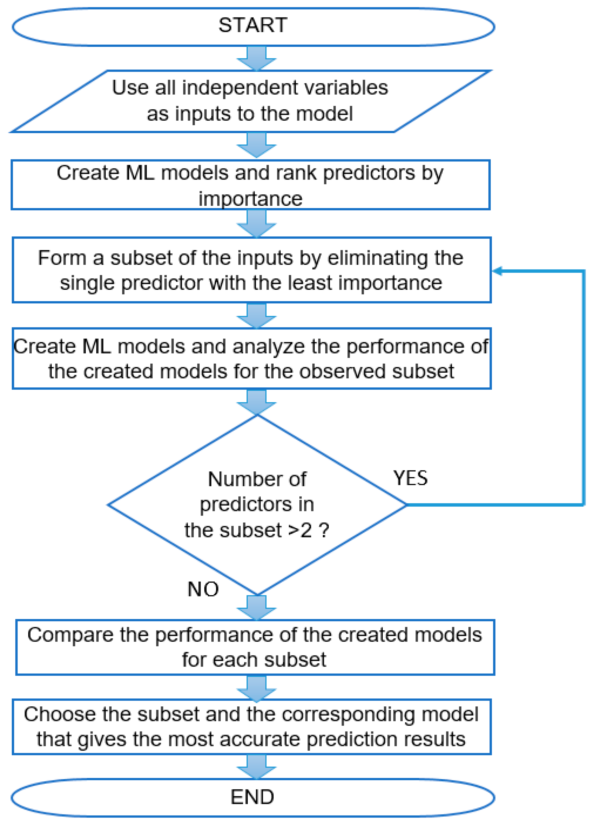
The application of the Wrapper technique for the selection of an optimal set of input variables in this research is based on the Backward selection via the recursive feature elimination algorithm, which was presented in [33]. In Figure 6, this algorithm is graphically represented by a flowchart. In the initial step, all 17 independent variables are used as inputs to the ML model, after which multiple predictive models are trained and tested. At the same time, it is necessary to determine the importance or influence of each predictor on the prediction results. In the next step, the input variable of least importance is eliminated, and the training and testing procedure is repeated over the subset obtained in this way, as well as the performance analysis of the solutions created. As long as the current subset of input variables consists of more than two inputs, it is necessary to eliminate individually each input variable with the next lowest importance from the ranked list, and so on. The elimination procedure is shown in a loop in Figure 6. When the input subset is reduced to two predictors, the performance of the created models is compared for each subset. Finally, for the optimal solution, the subset of inputs over which the most accurate predictive models were created is selected.
The performance of predictive models is measured with the Relative Error (RE) prediction criterion, for quality assessment and selection of the most accurate model. RE is calculated as the ratio of the sum of error squares of the dependent variable DEtoE and the sum of error squares of the null or intercept model:
R E = i = 1 n ( D E t o E i D P R E D i ) 2 i = 1 n ( D E t o E i D A V G i ) 2
where:
-
DEtoEi is a calculated end-to-end delay value for the i-th input/output vector,
-
DPREDi is a prediction value of DEtoEi, and
-
DAVGi is the arithmetic mean of the variable DEtoEi.

3.6. Optimization of a set of independent variables by the Pareto 80/20 rule

Another applied approach to optimization within the dimensionality reduction technique is the Pareto principle. Since optimality means the best combination of relevant factors, the Pareto principle is based on the strategic assumption that 80% of problems or effects in solutions come from 20% of causes. This is why it is often referred to as the "80/20 rule". The Pareto principle has proven its applicability in various fields, even though it has its roots in economics [34,35]. In this paper, on the basis of the created Pareto diagram, the optimal number of input variables is chosen so that their cumulative PI value is equal to or greater than 0.8 or 80%. For all alternative actions in predictive decision-making, available relevant information is used, and possible solutions for selecting one of the alternatives can be presented in matrix form. Machine learning is viewed as a multi-objective task. However, most often only one goal is observed - cost function optimization, or multiple objectives are aggregated into a scalar cost function. Using the Pareto principle to solve multi-objective tasks has proven to be one of the most effective approaches. In the Pareto-based approach to multi-objective optimization, the objective function is not a scalar value, but a vector. Therefore, several Pareto-optimal solutions are created instead of one, which can significantly improve the predictive performance of a model [36].

3.7. Creating predictive models using the ML method of automatic modeling

In the IBM SPSS Modeler software environment, optimized sets of predictors are brought to the input of the Auto Numeric node. Auto Numeric represents a method for automatic modeling where training and testing of multiple models is performed in just one step on the basis of different ML techniques: NN, classification and regression trees (C&R Tree), Chi Squared Automatic Interaction Detection (CHAID), linear regression, generalized linear regression, SVM [9]. As a result, the software analyzes the performance, ranks and offers the user the best solutions, and sorts the independent variables according to the importance of influence on the prediction results. Based on the aims and objectives of this research, three machine learning techniques are in focus: NN, k-NN and SVM [9,37].

3.8. Comparative analysis of prediction results and selection of the final model

The comparative analysis of the prediction results and the selection of the final model represents the last step in the research process. Based on the prediction performance expressed through the relative error criterion, one of the most accurate models is selected for each of the three observed approaches to optimizing the set of input variables. The main goal of this procedure is to test the statistical significance of the differences in prediction results for three ML models, i.e. for three approaches to predictor set optimization. Given that the same data set is used for testing in all three cases, the prediction results are compared using statistical methods, by the ANOVA test with Repeated Measures and the Friedman test.
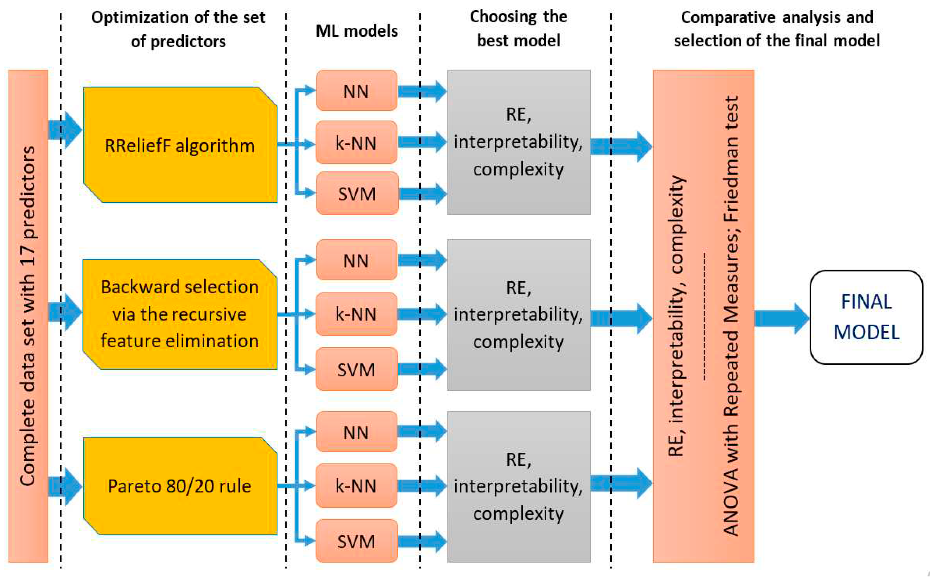
In addition to relative error, as one of the key indicators of prediction performance, special attention is paid to its complexity and interpretability when selecting an ML model [5]. Studies have shown that models with more complex ML algorithms are more difficult to interpret. The dimensionality of the space of input variables, and the complexity of the functions that the models need to learn, in addition to the algorithms, can affect the complexity of the model [5]. Figure 7 shows the methodological steps, from the optimization of the set of independent variables in each of the three investigated predictive models to the comparative analysis and selection of the final ML model.
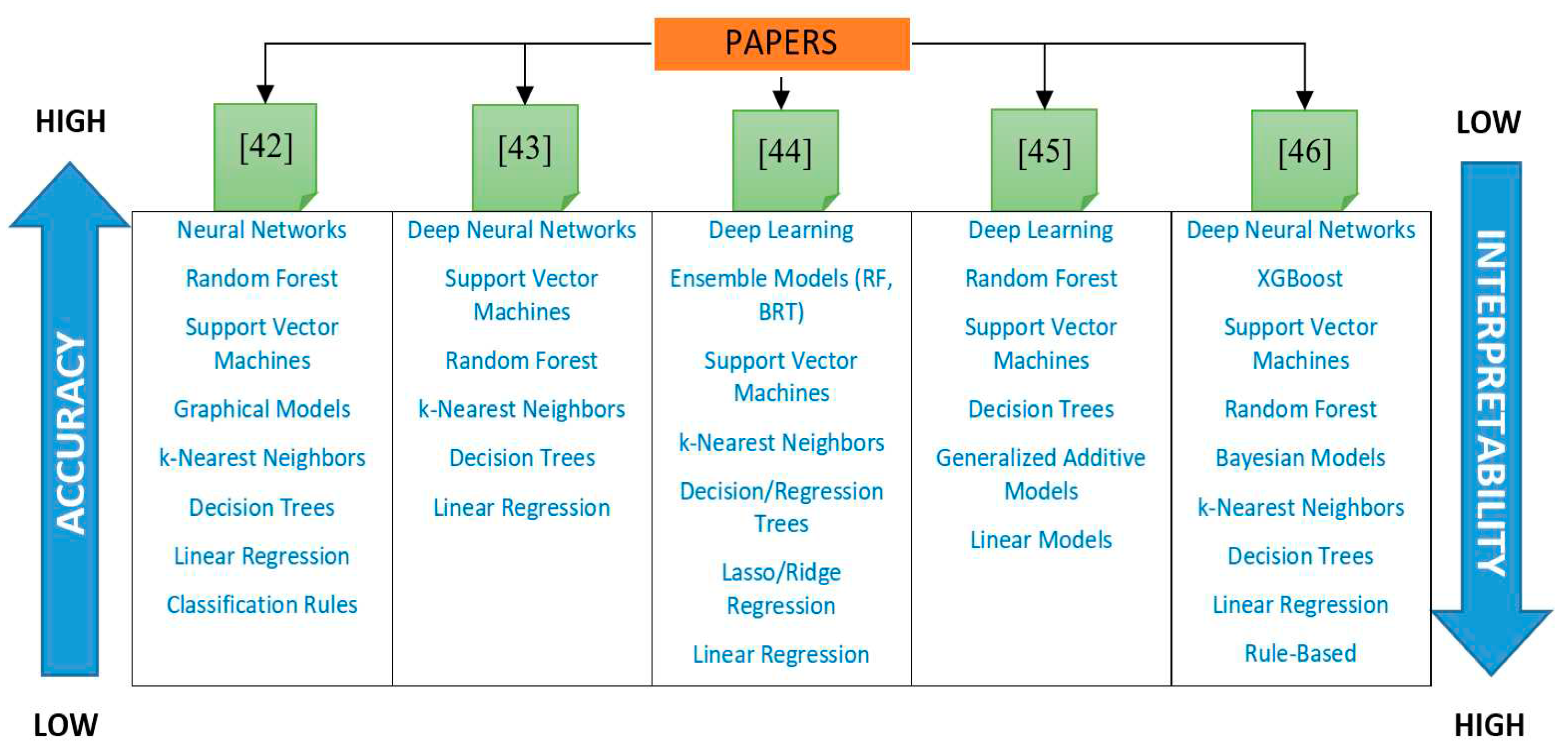
According to the results of numerous studies, priority is given to simpler, more interpretable solutions, although complex predictive models usually provide better performance [38,39,40]. In the paper [39], several definitions of the concept of interpretability are listed, among which the following stands out: "interpretability in ML is a degree to which a human can understand the cause of a decision from an ML model". For this reason, in recent years, a relatively new field, Interpretable Machine Learning (IML), has appeared. Within it, methods are investigated to transform ML models, the so-called black boxes, into white box models [5,39,41]. Figure 8 shows common models ranked according to accuracy and interpretability in relatively recent published research papers [42,43,44,45,46]. In the figure, the accuracy from the lowest to the highest value is given in a down-up orientation, while the interpretability with a growing trend is oriented in the Top-down direction.

4. Results and Discussion

4.1. Predictive ML models created over a set of predictors optimized by the RReliefF algorithm

The optimization results of the set of independent variables by the RReliefF algorithm for different values of k-Nearest Neighbors are shown in Table 3. For k=10, k=15 and k=20, the algorithm ranked the independent variables by weighting coefficients in the same tanking. The most influential predictor for all three cases is DL.16QAM.TB.Retrans, while Average_DL_User_Throughput is in last place with a negative weighting coefficient for each k.
According to expression (8), with the conventional value α=0.05 and the default value m=31143, the RT value is selected in the interval 0<RT<0.025. However, in practice, instead of a certain value of RT, and in accordance with the limitations, a few of the most important predictors that affect the prediction of the dependent variable are often chosen. Considering that, in the observed case, the number of variables with weighting coefficients greater than 0 is equal to 12, the first 6 ranked predictors, according to Table 3, are selected as the final number of inputs. The RT threshold value that can be set hypothetically, and which can correspond to this selection of the optimal set of variables is RT=0.0028.
Table 4 shows the ranked RE values and correlations for the three tested models that were created over the data set optimized by the RReliefF algorithm.
According to Table 4, the best predictive performance is shown by the model based on k-NN which has RE=0.109 and correlation coefficient equal to 0.944. That is why this model is selected as the best solution in the approach to predictor set optimization with the RReliefF algorithm. The SVM model has the highest relative error, which is RE=0.205, but also the lowest correlation value, which is equal to 0.893.

4.2. ML predictive models created over a set of predictors optimized by the Backward selection via the recursive feature elimination algorithm

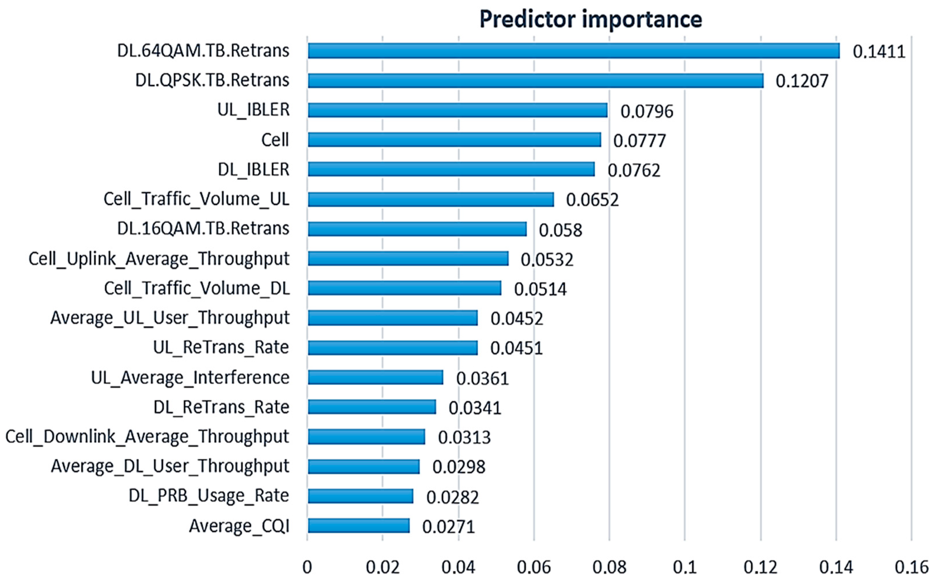
In accordance with the first step of the algorithm shown in Figure 6, all 17 independent variables are used as inputs to the ML models. Automatic training and testing of predictive models based on NN, SVM and k-NN techniques is performed using the Auto Numeric method in one pass through the modeling process. As one of the results of this step, Figure 9 shows the input variables ranked by PI value [47].
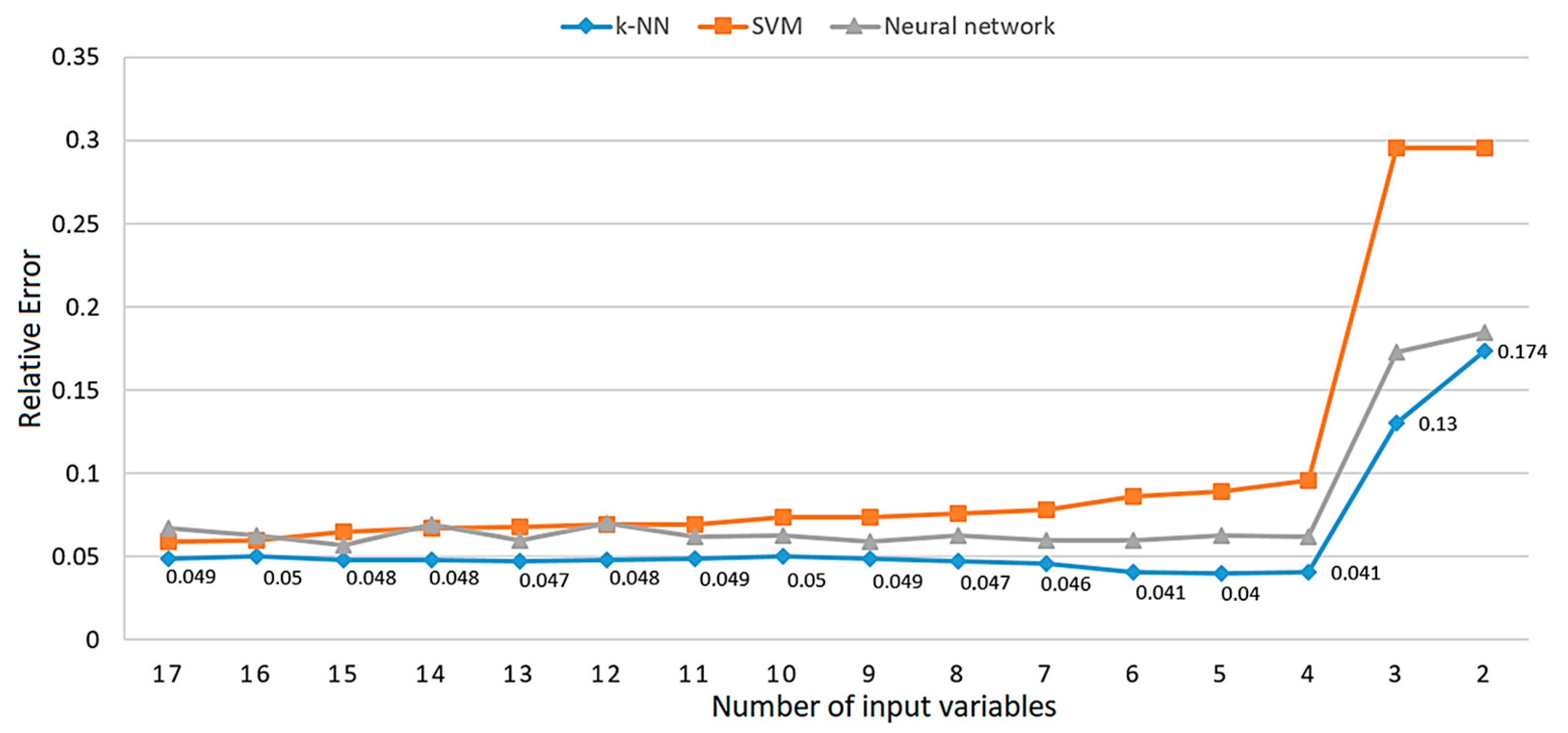
By multiple execution of the loop of the algorithm given in Figure 6, the RE values of the model testing are obtained, as shown in Figure 10. From the figure, it can be concluded that the best predictive performance is shown by the model based on k-NN, which has the smallest relative error (RE=0.04) for the five most influential input variables sorted according to Figure 10. Nevertheless, due to less complexity, the k-NN model with four inputs is selected as the best solution, and its relative error is slightly higher and amounts to RE=0.041. Also, it is evident that the prediction performance decreases drastically with a further reduction in the number of inputs to three and two variables.
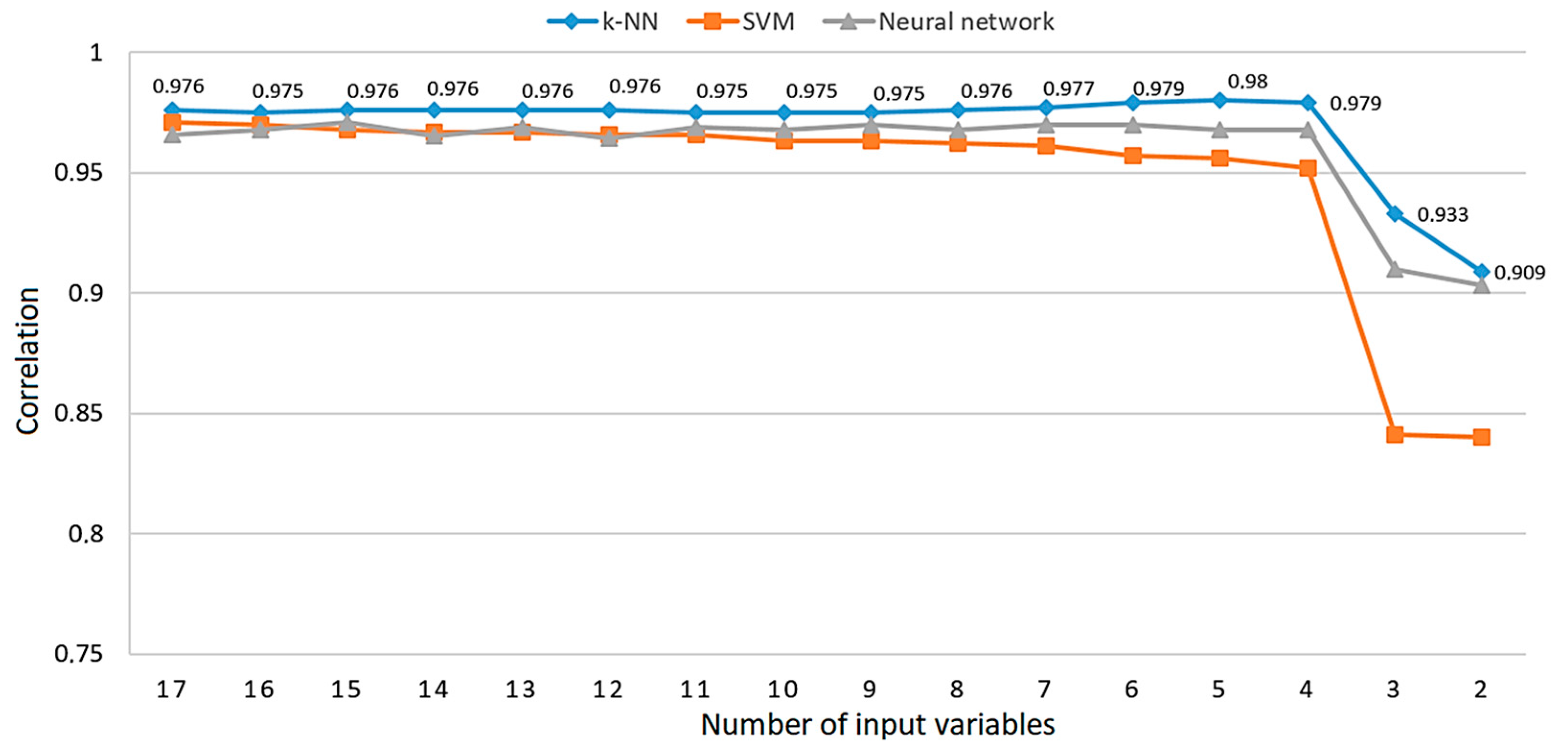
The performance of the tested predictive models, in addition to the relative error, can also be expressed by correlation, which is shown in Figure 11. It is concluded that the values of the Pearson correlation coefficients of the prediction results with the real data from the test set are "inverse" in relation to the RE values shown in Figure 10. Accordingly, the model with five inputs has the highest correlation coefficient (0.98), but due to the reasons mentioned above, the k-NN model with four inputs whose correlation coefficient is equal to 0.979 was selected as the best solution.

4.3. Predictive ML models created over a set of predictors optimized by the Pareto 80/20 rule

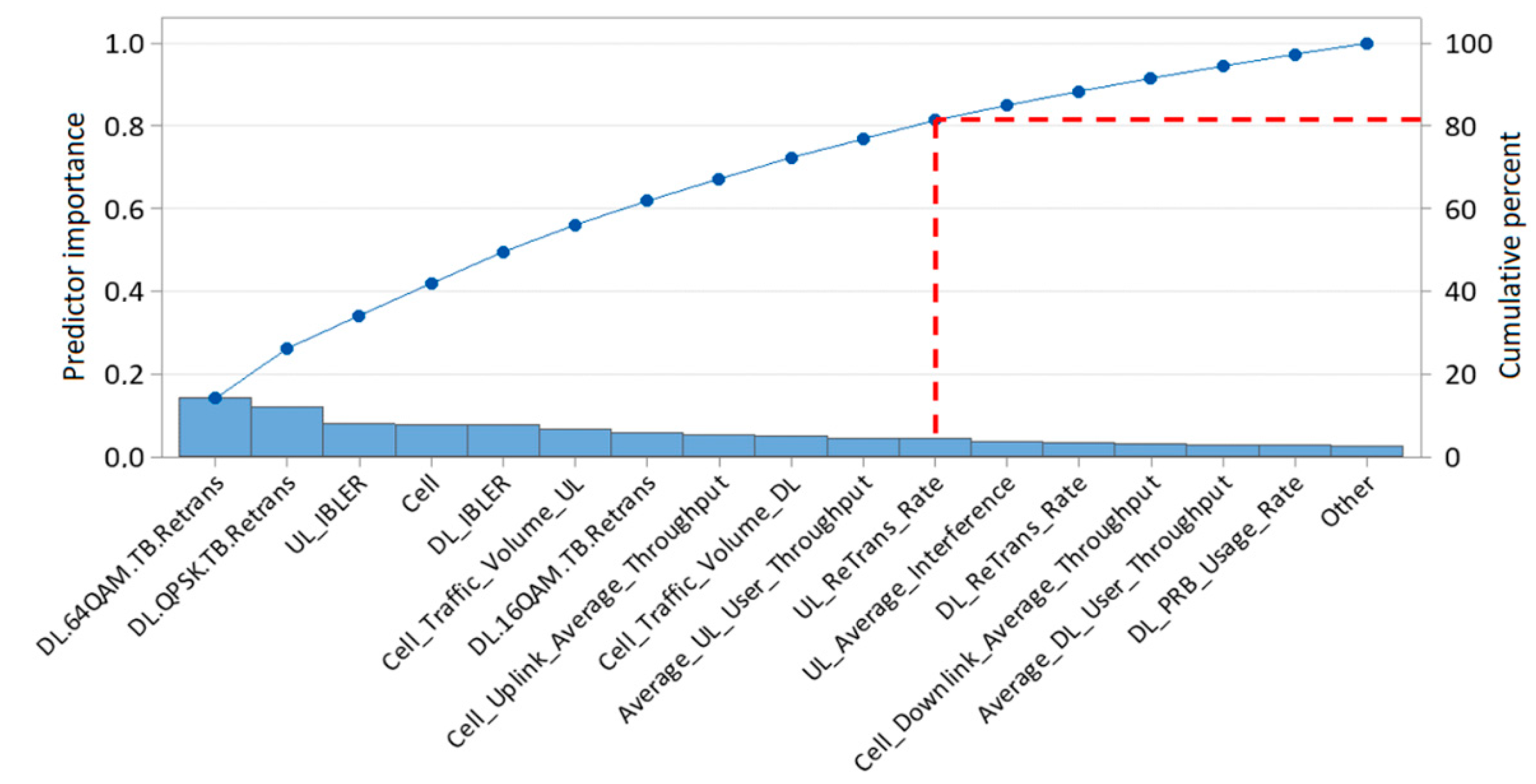
Figure 12 shows a Pareto diagram where the observed input variables are ordered according to the value of PI, from the highest to the lowest, by the ranking shown in Figure 9 [48]. The value of the cumulative curve for any input variable is equal to the sum of the PI values of individual predictors up to the observed variable, moving from the left to the right side of the diagram. According to the Pareto 80/20 rule, the goal is to find the first point on the curve with a cumulative value equal to or greater than 80%. This optimal point is marked in Figure 12, and the cumulative percentage in it is 81.34% for 11 input variables. According to the results shown in Figure 10, the k-NN model is selected as the best solution in this optimization approach, whose relative error at that point is RE=0.049, while the correlation is equal to 0.975 (Figure 11).

4.4. Comparative analysis of results using statistical methods and selection of the final model

Comparative analysis compares the delay prediction results of three ML models, each of which was selected as the best solution in one of the three observed approaches to optimizing the input set of variables. The main goal is to determine the statistical significance of the differences between the prediction results, which is the reason for testing the null hypothesis:
  • H0: µ1 = µ2 = µ3, where µ1, µ2 and µ3 are the arithmetic means of delay prediction values for k-NN models selected as the best solutions in the approach based on the RRelieff algorithm, Backward selection via the recursive feature elimination algorithm, and the Pareto 80/20 rule, respectively. In other words, this hypothesis represents the assumption that there are no significant statistical differences in the arithmetic means of the delay prediction results for the three observed models.
    In contrast, the alternative hypothesis can be stated as follows:
  • H1: There are significant statistical differences in the prediction results between at least two models, i.e. two optimization approaches.
The parametric statistical test that tests the null hypothesis is ANOVA with Repeated Measures [49]. However, it is first necessary to test one of the basic conditions for the application of this test, which is the normality of the distribution of the dependent variable in groups. The results of the Kolmogorov-Smirnov normality test for the observed models are given in Table 5.
The obtained significance value of the Sig. test for all three cases has the same value (Sig.=0.000). It means that the assumption about the normality of the distribution of the dependent variable in groups can be rejected. This conclusion can be confirmed graphically on the basis of the Q-Q plots shown in Figure 13. On the diagrams, it is obvious that there are significant deviations of the points from the line representing the normal distribution.
Given the non-fulfillment of the conditions from the aspect of normality of distribution, it is necessary to test the hypotheses with the Friedman test, which is a non-parametric alternative to ANOVA with Repeated Measures. Table 6 shows the results of the Friedman test performed in IBM SPSS Statistics [50]. In addition to the sample size (N), the test statistic (Chi-Square), degree of freedom (df) and significance level (Asymp. Sig.) are given in the table. Based on the value of Asymp. Sig., which is less than the α=0.05 level, it is concluded that there are statistically significant differences in the prediction results for the three models, i.e. for three approaches to optimizing the set of input variables.
The results given in Table 6 do not show the information for which pair of combined optimization techniques there is a significant statistical difference. The answer to this question is obtained with a Post Hoc statistical test. Table 7 shows the results of the Wilcoxon signed-rank post hoc test with the value of Z and Asymp. Sig. for each of the three combinations of approaches.
In order to interpret the results obtained, it is necessary to calculate the adjusted Bonferroni level of significance as the ratio of level α=0.05 and the number of pairs being compared, which as a result provides a value of 0.017. Given that Asymp. Sig.<0.017 applies to all combinations, it is concluded that there are statistically significant differences among the delay prediction results for all three pairs of approaches to optimizing the input set of variables.

5. Conclusions

For a long period of time, not only the amount of data, called BD, but also the number of users of network services and the range of user requests for higher QoS has been increasing drastically. Telecommunications operators face increasingly complex technical and technological problems in a domain of network traffic management, adequate planning and modern design of all dimensions of the quality of network resources, their allocation and performance - KPI, which is especially important for services such as VoIP and traffic streaming. Predictive modeling of required solutions currently is most often based on the techniques of the ML method. Numerous studies of different approaches to certain solutions for indicated problems are analyzed in this paper and presented in Section 2. Using the above and other experiences and theoretical findings of more comprehensive studies, the paper presents original approaches to predictive modeling of end-end delay of data packets through a real 4G LTE network in geo-space covered by the M:tel BL mobile operator with a focus on the area of a three-segment road in the road network of RS, BiH. In the LTE architecture, a total of 87 cells are located in the observed area, which provide users with a continuous and permanent network connection.
The paper has realized the aims and objectives of the research, from reducing the dimensionality of the space of input variables in the optimization model with Feature Selection techniques (RReliefF and Backward selection via the recursive feature elimination algorithms) and the Pareto 80/20 rule, through training and testing of ML models with NN, SVM and k-NN techniques with the selection of the best delay prediction model in the LTE network according to criteria of accuracy and complexity/interpretability to the implementation of a unique methodology of indirect assessment and calculation of dependent variable values based on the average number of active users in the network. At the same time, a universally applicable predictive model of delay in the LTE network, based on research in the real space of Big Data (BD) with input-output vectors, was created. The presented approaches to the optimization of the number of predictors by end-end delay modeling ML techniques in LTE networks by reducing the dimensions of BD and connecting independent variables in pairs with the calculation of KPI with the methodology of presenting and interpreting textual, algorithmic, graphic, photo-documentation, mathematical and computer-generated solutions, is in the opinion of the team of authors, a particularly important innovative contribution to the research of telecommunications traffic given in this paper. An optimal explanatory strategy was also used in creating a system of clarification of the presented methodology and results referring to similarities in the structure of what is being investigated in this paper with already known facts that, among other things, were published in cited papers and other authors' solutions. Also, familiar systems of relations that are used as models which can be useful to understand the new experience in the systematic scientific research of telecommunications traffic are taken into account, and the similarities created in analogies and hypotheses have led to the proven quality of the results presented.
The research results show that in all three approaches to the optimization of the input set of variables, the k-NN model is selected as the best solution. For the RReliefF optimization algorithm, the best model has 6 inputs and RE=0.109; for Backward selection via the recursive feature elimination algorithm, the best model has 4 inputs and RE=0.041; and for the Pareto 80/20 rule, the best model has 11 inputs and RE= 0.049. The comparative analysis of the results concludes that according to both observed criteria for the selection of the final model, the best solution is an approach to optimizing the number of predictors based on the Backward selection via the recursive feature elimination algorithm. In other words, the k-NN model created within this approach has the lowest RE value and the lowest number of input variables of all tested.

Author Contributions

Conceptualization, M.K.B., M.S. and M.V.; methodology, M.K.B. and M.S.; software, M.S. and M.V.; validation, M.K.B., D.N. and A.S.; formal analysis, M.K.B., D.N., M.S. and A.S.; investigation, M.K.B., M.S. and M.V.; resources, M.K.B., M.S., A.S., D.D. and G.P.; data curation, M.K.B., M.S., M.V. and D.D.; writing—original draft preparation, M.K.B. and M.S.; writing—review and editing, M.K.B., M.S. and M.V.; visualization, M.K.B., M.S., D.D. and G.P.; supervision, M.K.B. and M.S.; project administration, D.D, D.N., G.P. and M.V.; funding acquisition, D.D., G.P., A.S., D.N. and M.V. All authors have read and agreed to the published version of the manuscript.

Funding

This research received no external funding.

Institutional Review Board Statement

Not applicable.

Informed Consent Statement

Not applicable.

Data Availability Statement

The dataset is available upon request.

Acknowledgments

The authors gratefully acknowledge the mobile operator M:tel Banja Luka for their support by providing research data.

Conflicts of Interest

The authors declare no conflict of interest.

References

  1. Banjanin, M.K.; Maričić, G.; Stojčić, M. Multifactor Influences on the Quality of Experience Service Users of Telecommunication Providers in the Republic of Srpska, Bosnia and Herzegovina. International Journal for Quality Research 2022, 17, 369–386. [Google Scholar] [CrossRef]
  2. Banjanin, M.K.; Stojčić, M.; Danilović, D.; Ćurguz, Z.; Vasiljević, M.; Puzić, G. Classification and Prediction of Sustainable Quality of Experience of Telecommunication Service Users Using Machine Learning Models. Sustainability 2022, 14, 17053. [Google Scholar] [CrossRef]
  3. Mesbahi, N.; Dahmouni, H. Delay and jitter analysis in LTE networks. In Proceedings of the 2016 International Conference on Wireless Networks and Mobile Communications (WINCOM), Fez, Morocco, 26-29 October 2016; IEEE; pp. 122–126. [Google Scholar] [CrossRef]
  4. Yaqoob, J.I.A.Y.; Pang, W.L.; Wong, S.K.; Chan, K.Y. Enhanced exponential rule scheduling algorithm for real-time traffic in LTE network. International Journal of Electrical and Computer Engineering (IJECE) 2020, 10, 1993–2002. [Google Scholar] [CrossRef]
  5. Stojčić, M.; Banjanin, M.K.; Vasiljević, M.; Stjepanović, A.; Ćurguz, Z. PCA modeling of extraction and selection of variables influencing LTE network delay in urban mobility conditions. Paper presented at International Conference on Advances in Traffic and Communication Technologies ATCT 2023, Sarajevo, Bosnia and Herzegovina., 11-12 May 2023. [Google Scholar]
  6. ETSI TS 123 107 v12.0.0; Digital cellular telecommunications system (Phase 2+); Universal Mobile Telecommunications System (UMTS); LTE.; Quality of Service (QoS) concept and architecture. European Telecommunications Standards Institute: Sophia Antipolis Cedex, France, 2014. Available online: https://www.etsi.org/deliver/etsi_ts/123100_123199/123107/12.00.00_60/ts_123107v120000p.pdf (accessed on 26 June 2023).
  7. Kumar, V.; Minz, S. Feature selection: A literature review. SmartCR 2014, 4, 211–229. [Google Scholar] [CrossRef]
  8. Cai, J.; Luo, J.; Wang, S.; Yang, S. Feature selection in machine learning: A new perspective. Neurocomputing 2018, 300, 70–79. [Google Scholar] [CrossRef]
  9. Đukić, A.; Bjelošević, R.; Stojčić, M.; Banjanin, M.K. Network Model of Multiagent Communication of Traffic Inspection for Supervision and Control of Passenger Transportation in Road and City Traffic. In Proceedings of the Croatian Society for Information, Communication and Electronic Technology – MIPRO 2023 46th (Hybrid) Convention, Opatija, Croatia, 22-26 May 2023; pp. 1352–1357. [Google Scholar]
  10. Torres-Figueroa, L.; Schepker, H.F.; Jiru, J. QoS evaluation and prediction for C-V2X communication in commercially-deployed LTE and mobile edge networks. In Proceedings of the 2020 IEEE 91st Vehicular Technology Conference (VTC2020-Spring), Antwerp, Belgium, 25-28 May 2020; IEEE; pp. 1–7. [Google Scholar] [CrossRef]
  11. Zhang, W.; Feng, M.; Krunz, M.; Volos, H. Latency prediction for delay-sensitive v2x applications in mobile cloud/edge computing systems. In Proceedings of the GLOBECOM 2020-2020 IEEE Global Communications Conference, Taipei, Taiwan, 7-11 December 2020; IEEE; pp. 1–6. [Google Scholar] [CrossRef]
  12. Brown, J.; Khan, J.Y. A predictive resource allocation algorithm in the LTE uplink for event based M2M applications. IEEE Transactions on Mobile Computing 2015, 14, 2433–2446. [Google Scholar] [CrossRef]
  13. Khatouni, A.S.; Soro, F.; Giordano, D. A machine learning application for latency prediction in operational 4g networks. In In Proceedings of the 2019 IFIP/IEEE Symposium on Integrated Network and Service Management (IM), Arlington, VA, USA, 8-12 April 2019; IEEE; pp. 71–74. [Google Scholar]
  14. Zhohov, R.; Minovski, D.; Johansson, P.; Andersson, K. Real-time performance evaluation of LTE for IIoT. In Proceedings of the 2018 IEEE 43rd Conference on Local Computer Networks (LCN), Chicago, IL, USA, 1-4 October 2018; IEEE; pp. 623–631. [Google Scholar] [CrossRef]
  15. Lai, W.K.; Tang, C.L. QoS-aware downlink packet scheduling for LTE networks. Computer Networks 2013, 57, 1689–1698. [Google Scholar] [CrossRef]
  16. Lai, W.K.; Hsu, C.W.; Kuo, T.H.; Lin, M.T. A LTE downlink scheduling mechanism with the prediction of packet delay. In Proceedings of the 2015 Seventh International Conference on Ubiquitous and Future Networks, Sapporo, Japan, 7-10 July 2015; IEEE; pp. 257–262. [Google Scholar] [CrossRef]
  17. Nasri, M.; Hamdi, M. LTE QoS parameters prediction using multivariate linear regression algorithm. In Proceedings of the 2019 22nd conference on innovation in clouds, internet and networks and workshops (ICIN), Paris, France, 19-21 February 2019; IEEE; pp. 145–150. [Google Scholar] [CrossRef]
  18. Ahmed, A.H.; Hicks, S.; Riegler, M.A.; Elmokashfi, A. Predicting High Delays in Mobile Broadband Networks. IEEE Access 2021, 9, 168999–169013. [Google Scholar] [CrossRef]
  19. Banjanin, M.K.; Stojčić, M.; Drajić, D.; Ćurguz, Z.; Milanović, Z.; Stjepanović, A. Adaptive Modeling of Prediction of Telecommunications Network Throughput Performances in the Domain of Motorway Coverage. Applied Sciences 2021, 11, 3559. [Google Scholar] [CrossRef]
  20. Loshakov, V.A.; Al-Janabi, H.D.; Al-Zayadi, H.K. Adaptive control signal parameters in LTE technology with MIMO. Telecommunications Problems 2012, 2, 78–90, UDC 621.396. http://openarchive.nure.ua/handle/document/430.
  21. Ren, J.; Zhang, X.; Xin, Y. Using Deep Convolutional Neural Network to Recognize LTE Uplink Interference. In Proceedings of the 2019 IEEE Wireless Communications and Networking Conference (WCNC), Marrakesh, Morocco, 15-18 April 2019; IEEE; pp. 1–6. [Google Scholar] [CrossRef]
  22. Madi, N.K.; Hanapi, Z.M.; Othman, M.; Subramaniam, S.K. Delay-based and QoS-aware packet scheduling for RT and NRT multimedia services in LTE downlink systems. EURASIP Journal on Wireless Communications and Networking 2018, 180, 1–21. [Google Scholar] [CrossRef]
  23. Kuhn, M.; Johnson, K. Feature Engineering and Selection: A Practical Approach for Predictive Models, 1st ed.; Chapman and Hall/CRC: Boca Raton, Florida, 2019; ISBN 978-1-13-807922-9. [Google Scholar]
  24. Li, J.; Cheng, K.; Wang, S.; Morstatter, F.; Trevino, R.P.; Tang, J.; Liu, H. Feature selection: A data perspective. ACM computing surveys (CSUR) 2017, 50, 1–45. [Google Scholar] [CrossRef]
  25. Wah, Y.B.; Ibrahim, N.; Hamid, H.A.; Abdul-Rahman, S.; Fong, S. Feature Selection Methods: Case of Filter and Wrapper Approaches for Maximising Classification Accuracy. Pertanika Journal of Science & Technology 2018, 26, 329–340. [Google Scholar]
  26. MathWorks. Introduction to Feature Selection. Available online: https://www.mathworks.com/help/stats/feature-selection.html (accessed on 27 March 2023).
  27. Kira, K.; Rendell, L.A. A practical approach to feature selection. In Proceedings of the Machine learning proceedings, Aberdeen, Scotland, 1-3 July 1992; pp. 249–256. [Google Scholar] [CrossRef]
  28. Kira, K.; Rendell, L.A. The feature selection problem: Traditional methods and a new algorithm. In Proceedings of the tenth national conference on Artificial intelligence - AAAI ’92, San Jose, California, 12-16 July 1992; pp. 129–134. [Google Scholar]
  29. Kononenko, I. Estimating Attributes: Analysis and extensions of RELIEF. In Machine Learning: ECML-94; Bergadano, F., De Raedt, L., Eds.; Springer: Berlin/Heidelberg, Germany, 1994; Volume 784. [Google Scholar] [CrossRef]
  30. Robnik-Šikonja, M.; Kononenko, I. An adaptation of Relief for attribute estimation in regression. In Proceedings of the Machine learning: Proceedings of the fourteenth international conference (ICML’97), Nashville, Tennessee, USA, 8-12 July 1997; pp. 296–304.
  31. MathWorks. Relief. Available online: https://www.mathworks.com/help/stats/relieff.html (accessed on 24 April 2023).
  32. Urbanowicz, R.J.; Meeker, M.; La Cava, W.; Olson, R.S.; Moore, J.H. Relief-based feature selection: Introduction and review. Journal of biomedical informatics 2018, 85, 189–203. [Google Scholar] [CrossRef] [PubMed]
  33. Guyon, I.; Weston, J.; Barnhill, S.; Vapnik, V. Gene selection for cancer classification using support vector machines. Machine learning 2002, 46, 389–422. [Google Scholar] [CrossRef]
  34. Okorie, O.; Salonitis, K.; Charnley, F.; Turner, C. A systems dynamics enabled real-time efficiency for fuel cell data-driven remanufacturing. Journal of Manufacturing and Materials Processing 2018, 2, 77. [Google Scholar] [CrossRef]
  35. Hugh, J. Engineering Design, Planning, and Management, 2nd ed.; Academic Press: Cambridge, Massachusetts, United States, 2021; ISBN 978-0-12-821055-0. [Google Scholar]
  36. Jin, Y.; Sendhoff, B. Pareto-based multiobjective machine learning: An overview and case studies. IEEE Transactions on Systems, Man, and Cybernetics, Part C (Applications and Reviews) 2008, 38, 397–415. [Google Scholar] [CrossRef]
  37. Lee, S.H.; Mazumder, J.; Park, J.; Kim, S. Ranked feature-based laser material processing monitoring and defect diagnosis using k-NN and SVM. Journal of Manufacturing Processes 2020, 55, 307–316. [Google Scholar] [CrossRef]
  38. Ahmad, M.A.; Eckert, C.; Teredesai, A. Interpretable machine learning in healthcare. In Proceedings of the 2018 ACM international conference on bioinformatics, computational biology, and health informatics, Washington DC, USA, 29 August-1 September 2018; pp. 559–560. [Google Scholar]
  39. Abdullah, T.A.; Zahid, M.S.M.; Ali, W. A review of interpretable ML in healthcare: Taxonomy, applications, challenges, and future directions. Symmetry 2021, 13, 2439. [Google Scholar] [CrossRef]
  40. Dherin, B.; Munn, M.; Rosca, M.; Barrett, D. Why neural networks find simple solutions: The many regularizers of geometric complexity. In Proceedings of the Thirty-sixth Conference on Neural Information Processing Systems-NeurIPS, New Orleans Convention Center, USA, 28 November–9 December 2022; Volume 35, pp. 2333–2349. [Google Scholar]
  41. Stiglic, G.; Kocbek, P.; Fijacko, N.; Zitnik, M.; Verbert, K.; Cilar, L. Interpretability of machine learning-based prediction models in healthcare. Wiley Interdisciplinary Reviews: Data Mining and Knowledge Discovery 2020, 10, e1379. [Google Scholar] [CrossRef]
  42. Morocho-Cayamcela, M.E.; Lee, H.; Lim, W. Machine learning for 5G/B5G mobile and wireless communications: Potential, limitations, and future directions. IEEE access 2019, 7, 137184–137206. [Google Scholar] [CrossRef]
  43. Yang, Y.J.; Bang, C.S. Application of artificial intelligence in gastroenterology. World journal of gastroenterology 2019, 25, 1666. [Google Scholar] [CrossRef] [PubMed]
  44. Pichler, M.; Hartig, F. Machine learning and deep learning—A review for ecologists. Methods in Ecology and Evolution 2023, 14, 994–1016. [Google Scholar] [CrossRef]
  45. Guo, M.; Zhang, Q.; Liao, X.; Chen, Y. An interpretable machine learning framework for modelling human decision behavior. arXiv preprint 2019, arXiv:1906.01233. [Google Scholar]
  46. Nesvijevskaia, A.; Ouillade, S.; Guilmin, P.; Zucker, J.D. The accuracy versus interpretability trade-off in fraud detection model. Data & Policy 2021, 3, e12. [Google Scholar] [CrossRef]
  47. Chowdhury, M.Z.I.; Turin, T.C. Variable selection strategies and its importance in clinical prediction modelling. Family medicine and community health 2020, 8, e000262. [Google Scholar] [CrossRef]
  48. Wang, J.; Jiang, C.; Zhang, H.; Ren, Y.; Chen, K.C.; Hanzo, L. Thirty years of machine learning: The road to Pareto-optimal wireless networks. IEEE Communications Surveys & Tutorials 2020, 22, 1472–1514. [Google Scholar] [CrossRef]
  49. Yu, Z.; Guindani, M.; Grieco, S.F.; Chen, L.; Holmes, T.C.; Xu, X. Beyond t test and ANOVA: Applications of mixed-effects models for more rigorous statistical analysis in neuroscience research. Neuron 2022, 110, 21–35. [Google Scholar] [CrossRef]
  50. Balali, A.; Valipour, A. Identification and selection of building façade's smart materials according to sustainable development goals. Sustainable Materials and Technologies 2020, 26, e00213. [Google Scholar] [CrossRef]
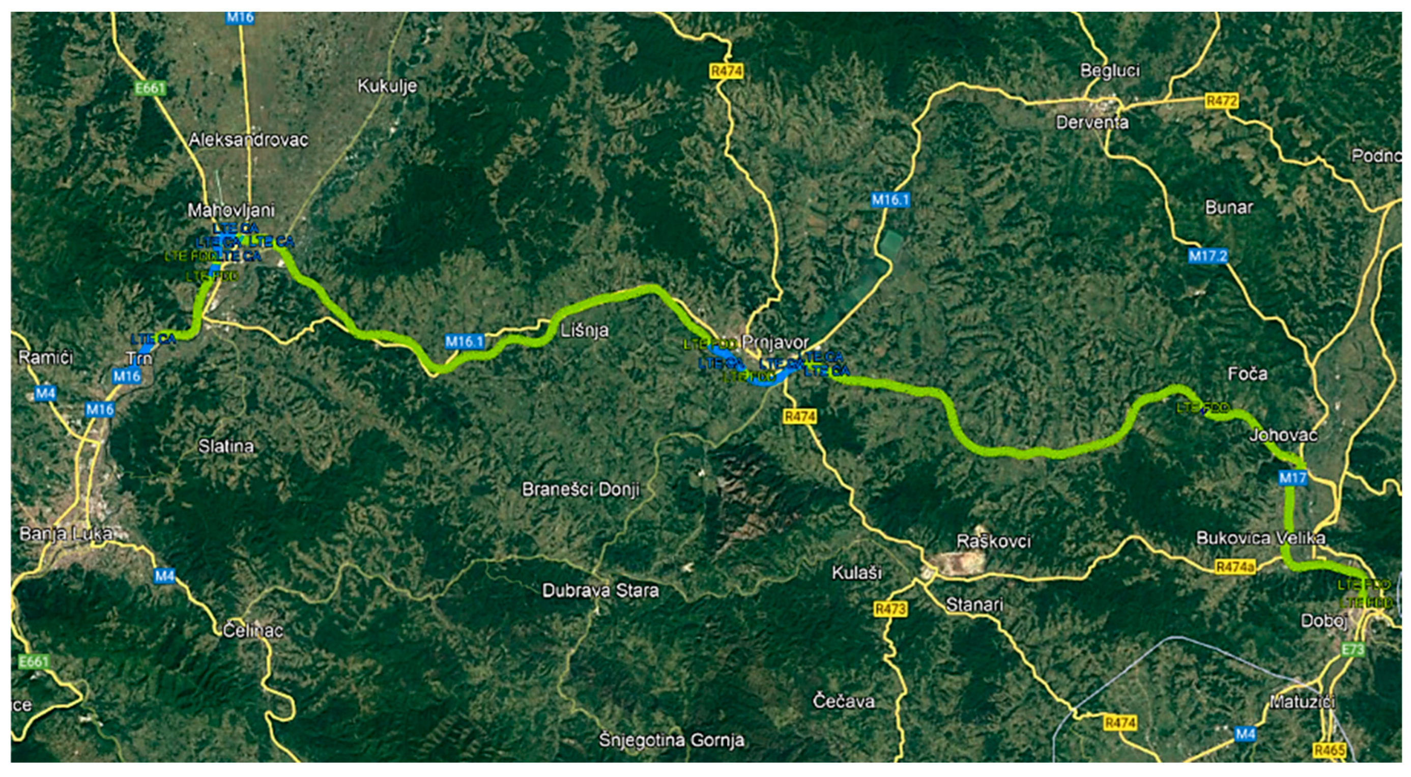
Figure 1. Geographical area of research.
Preprints 78089 g001
Figure 2. Layout of eNodeB locations with marked signal propagation in the research area.
Preprints 78089 g002
Figure 3. Average values of end-to-end delay of VoIP services calculated for EXP-RULE, EXP-PF, PPM and DQAS scheduling algorithms and for mobile user movement speed of 120 km/h.
Preprints 78089 g003
Figure 4. Method of calculating the values of the dependent variable DEtoE.
Preprints 78089 g004
Figure 5. Histogram of the dependent variable DEtoE.
Preprints 78089 g005
Figure 6. Backward selection via the recursive feature elimination algorithm to optimize the number of predictors.
Preprints 78089 g006
Figure 7. Steps of the methodological procedure from the optimization of the set of predictors to the selection of the final model
Preprints 78089 g007
Figure 8. ML models ranked by accuracy and interpretability in various published research papers.
Preprints 78089 g008
Figure 9. Independent variables ranked by PI.
Preprints 78089 g009
Figure 10. Relative error of ML models testing.
Preprints 78089 g010
Figure 11. Correlation of ML models prediction results with data test set.
Preprints 78089 g011
Figure 12. Pareto diagram for predictor set optimization.
Preprints 78089 g012
Figure 13. Normality tests of delay prediction results: a) RReliefF algorithm; b) Backward selection via the recursive feature elimination algorithm; c) Pareto 80/20 rule.
Preprints 78089 g013
Table 1. Overview of important criteria in relevant published research papers
Ref. No. Models and techniques Regression/
Classification
Service/
Application
Dimensionality reduction methods and techniques
[10] NN, Recurrent Neural Network (RNN) with Long Short-Term Memory (LSTM) neurons, Random Forest (RF),
SVM
Classification C-V2X Maximum Dependency (MD) algorithm
[11] LSTM;
k-medoids classification,
Epanechnikov Kerne,
Moving average functions
Regression and
Classification
Delay-sensitive V2X
Applications in Mobile Cloud/Edge Computing Systems
-
[12] Mathematical models Regression M2M uplink communication -
[13] Logistic Regression (LR), SVM, Decision Tree (DT) Classification Operational 4G Networks Services Random Forest
[14] Artificial Neural Networks, Decision Tree, Ensemble modeling: Bagging technique with a Decision Tree Regression IIoT Lag features, Window features
[15] Mathematical models, PPM, virtual queues Regression Real time services -
[16] Mathematical models, PPM, virtual queues Regression Real time services -
[17] Multivariate linear regression technique Regression LTE services -
[18] Logistic regression, Random forest, Light gradient-boosting machine (LightGBM), Ensemble Classification 4G and 5G services -
Table 2. Descriptive statistics for the dependent variable DEtoE
Mean StDev Var Min Median Max Skewness Kurtosis
4.1503 2.6520 7.0329 1.8081 3.2516 25.8282 2.81 10.17
Table 3. Optimization results of the set of independent variables by the RReliefF algorithm
Rank Independent variable or Predictor Predictor weighting coefficients for individual values of k
k=10 k=15 k=20
1 DL.16QAM.TB.Retrans 0.0061 0.0065 0.007
2 DL.QPSK.TB.Retrans 0.006 0.0064 0.0067
3 Cell_Traffic_Volume_UL 0.0041 0.0044 0.0045
4 DL_PRB_Usage_Rate 0.0037 0.004 0.0043
5 Cell_Traffic_Volume_DL 0.0033 0.0035 0.0038
6 UL_Average_Interference 0.0028 0.0031 0.0033
7 DL.64QAM.TB.Retrans 0.0027 0.0028 0.0029
8 Cell 0.0024 0.0025 0.0027
9 UL_IBLER 0.001 0.001 0.0012
10 UL_ReTrans_Rate 0.0009 0.001 0.0011
11 Cell_Uplink_Average_Throughput 0.0006 0.0006 0.0007
12 Average_UL_User_Throughput 0.0001 0.0001 0.0001
13 Average_CQI -0.0008 -0.0008 -0.0009
14 DL_ReTrans_Rate -0.0013 -0.0013 -0.0014
15 DL_IBLER -0.0015 -0.0016 -0.0017
16 Cell_Downlink_Average_Throughput -0.0019 -0.002 -0.0021
17 Average_DL_User_Throughput -0.0027 -0.0029 -0.003
Table 4. Results of testing the models created over the data set optimized by the RReliefF algorithm.
Model RE Correlation
1. k-NN 0.109 0.944
2. NN 0.159 0.917
3. SVM 0.205 0.893
Table 5. Tests of Normality with summarized optimization and prediction results.
An approach to optimization of a set of input variables ML model selected Number of inputs RE Kolmogorov-Smirnov
Statistic df Sig.
RReliefF algorithm k-NN 6 0.109 0.188 31143 0.000
Backward selection via the recursive feature elimination algorithm k-NN 4 0.041 0.191 31143 0.000
Pareto 80/20 rule k-NN 11 0.049 0.189 31143 0.000
Table 6. Results of the Friedman test.
N 31143
Chi-Square 268.019
df 2
Asymp. Sig. 0.000
Table 7. Wilcoxon signed-rank post hoc test results.
Pairs for comparison
RReliefF - Pareto 80/20 rule Backward selection via the recursive feature elimination - RReliefF Backward selection via the recursive feature elimination - Pareto 80/20 rule
Z -3.077 -7.848 -18.727
Asymp. Sig. (2-tailed) 0.002 0.000 0.000
Disclaimer/Publisher’s Note: The statements, opinions and data contained in all publications are solely those of the individual author(s) and contributor(s) and not of MDPI and/or the editor(s). MDPI and/or the editor(s) disclaim responsibility for any injury to people or property resulting from any ideas, methods, instructions or products referred to in the content.
Copyright: This open access article is published under a Creative Commons CC BY 4.0 license, which permit the free download, distribution, and reuse, provided that the author and preprint are cited in any reuse.
Prerpints.org logo

Preprints.org is a free preprint server supported by MDPI in Basel, Switzerland.

Subscribe

© 2024 MDPI (Basel, Switzerland) unless otherwise stated