
Submitted:
28 June 2023
Posted:
30 June 2023
Read the latest preprint version here
Abstract
Accurate measurement of solid precipitation (S) has a critical importance for proper understanding of the Earth’s hydrological cycle, validation of emerging technologies and weather prediction models, and developing parameterizations of severe weather elements such as visibility (Vis). However, measuring S is still a challenging problem mainly because of wind effects. The wind effects are normally mitigated by using a Double-Fence Automated Reference (DFAR) system to reduce the wind speed (Ug). To contribute towards addressing some of these issues we have analyzed data sets collected at a site located in Southern Ontario, Canada using several instruments. The instruments include two Geonor gauges, one placed inside a DFAR (SDFAR) and the other inside a double Alter shield (DASG), a Pluvio2 gauge inside a single Alter shield (SASP), a HotPlate, a PARSIVEL2 Disdrometer that measures S and fall velocity (V), and a FD12P senor that measures S and type and Vis. The results show that for the Ug observed in this study (Ug < 6 ms-1), both DASG and SASP have similar collection efficiency (CE) of near 70%. The transfer functions (TF) for DASG and SASP as a function of Ug and also Ug, and V have been derived. The TF for the DASG that includes both Ug and V showed better agreement with observation than just Ug alone. The S measured using all the other instruments were correlated well with SDFAR, but the PARSIVEL2 and FD12P overestimated and underestimated the snow amount respectively as compared the SDFAR. However, the HotPlate captured similar amount of S as the SDFAR. According to this study, the SDFAR showed good correlation with Vis.
Keywords:
solid precipitation and type measurements
; solid precipitation catch efficiency
; snow gauges
; non-traditional solid precipitation censors
; visibility in snow
; aviation
1. Introduction
Accurate measurement of solid precipitation (S) is critical for understanding of the hydrological cycle and validation of numerical weather prediction (NWP) models, particularly for severe weather forecasting and nowcasting applications that are relevant for aviation and ground transportation. Reduction of visibility due to snow is one of the major causes of aviation related delays (Ballesteros and Hitchens, 2018) and ground transportation accidents (Das et al. 2018; Eisenberg and Warner, 2005). In fact, solid precipitation intensity is estimated based on visibility, particularly for aviation application (Rasmussen et al., 1999; Boudala and Isaac, 2009). Many of the current NWP models parameterize visibility in terms of S (Rasmussen et al., 1999, Boudala and Isaac, 2009; Gultepe et al., 2010). These parameterizations were mainly developed based on low resolution (e.g., hourly, daily) manually determined S or non-standard snow gauge data. Developing a better parametrization is challenging due to the difficulty associated with characterization of scattering properties of snow particles (Rasmussen et al. 1999, Boudala and Isaac, 2009, Falconi et al., 2018).
One of the ways to mitigate the effects of wind speed that normally diminishes the catch efficiency of many traditional snow gauges use a standard wind shied referred to as Double Fence Intercomparison Reference (DFIR) as recommended by the World Meteorological Organization (WMO) (Goodison et al, 1998) (see Figure 1). Using this as a reference, correction or adjustment factors normally referred to as transfer functions of various precipitation gauges without or with shields (single or double Alter) can be developed. Previously these transfer functions were derived based on coarse time resolution data (e.g. daily accumulated precipitation data) (Goodison et al, 1998; Goodison and Yang, 1995). Currently there are a number of studies of solid precipitation catch efficiency of automated Geonor or Pluvio2 gauge with a single Alter shield configuration set to collect data at high temporal resolution (e.g., Kochendorfer et al., 2017; 2022 Smith and Yang, 2010). These studies are also mainly related to the effects of wind speed normally captured using some type of adjustment or transfer functions as summarized in recent papers (e.g., Kochendorfer et al. 2022, Zhang et al., 2022; Pierre et al., 2019). There are, however, relatively limited studies of catch efficiency of the automated Geonor with double Alter shield configuration (e.g., Rasmussen et al, 2012). Furthermore, although Some studies also include the effect of temperature (Kochendorfer et al., 2017; Køltzow et al., 2021), the catch efficiency or transfer functions that explicitly consider other parameters such as fall velocity are also limited in literature, particularly based on in-situ measurements (Colli et al., 2020, Leroux et al., 2021, Hoover et al., 2021).
In this paper, high-resolution solid precipitation data collected using an automated Geonor gauge placed inside an orthogonal double fence normally referred to as Double Fence Automated Reference (DFAR ) is used to develop and test new transfer functions for Geonor gauge with a double Alter shield and OTT Pluvio2 gauge with a single Alter shield. The transfer functions are developed based on both wind speed and fall velocity and wind speed alone. A number of non-traditional precipitation sensors were also evaluated using the DFAR data. By taking advantage of the DFAR solid precipitation intensity data, new visibility parameterizations are also developed and compared against the one found in literature. The paper is organized as follows: The material and methods are discussed in Section 2, the results are presented in Section 3 and the conclusions are given in Section 4.
2. Materials and Methods
2.1. The Geonor T-200B3 and OTT Pluvio2 Gauge Data Analysis
The Plivio2 and Geonor gauge data used in this study is mainly based on data collected during 2012-2013 period at the Centre for Atmospheric Research Experiment (CARE) site located at the Southern Ontario, Canada as part of the Solid Precipitation Intercomparison Experiment (SPICE) project (Nitu et al., 2018). The solid precipitation rate or accumulation being discussed in this paper is defined as liquid water equivalent (LWE) (Boudala et al., 2017; Rasmussen et al., 2012). The Geonor T-200B3 precipitation gauge used in this study is described in many publications including (Nitu et al., 2012; Smith et al., 2020; Leroux et al., 2021; Kochendorfer et al., 2017, Rasmussen et al., 2012). The instrument employs three transducers/wires combinations for precipitation accumulation measurements. The transducers cause the wires to vibrate and their vibrational frequency measurements are used to determine the depth through a frequency-dependent quadratic equation and this is converted to liquid equivalent solid precipitation. The Geonor gauge with a single Alter shield was installed at 3 m height inside an orthogonal double fence, the DFAR as shown in Figure 1 to minimize the effect of wind. The raw data contains precipitation accumulation corresponding to each wire calculated at 6 seconds time intervals. At such a high temporal resolution, the Geonor raw data can be quite noisy even with reduced wind effects, particularly under clear and light precipitation conditions, and hence requires careful assessment of each data set. For this study we have selected 23 mostly snow days based on measurements of present weather sensors. The algorithm used for data analysis is described in Boudala et al., (2016). The first step is removing any suspicious artifacts in the data using some reasonable thresholds. After removing the artifact, the data is de-noised using coefficients of Gaussian low-pass filter and Matlab zero-phase forward and reverse digital filtering method. The digitally filtered data is assessed for possible false precipitation events using the FD12P probe and if found they are removed from the data. The average of the three wires was used unless one of the wires is deviated from the mean by twice the minimum standard deviation of one of the wires (see Boudala et al., 2016). For precipitation type, wind speed and temperature studies, 10 min averaged data was used and for the catch efficiency study, 30 min averaged data was used and the precipitation data less than 0.2 mmh-1 have been ignored.
The physical description and operating principles of the OTT Pluvio2 200 gauge used in this study is also described in SPICE reports (Nitu et al., 2012 ; Nitu et al., 2018). The gauge has a sampling area of 200 cm2 and collection capacity of 1500 mm. The operating principle is based on collecting the precipitation particle in bucket and weighing the content using a high-precision stainless steel load cell. The load cell is hermetically sealed in order to be protected from unwanted environmental effects. The sampling resolution was 6 seconds similar to the Geonor data. The accumulated total non-real time liquid equivalent solid precipitation was used and processed the same as the Geonor data described earlier. The functional form of the collection efficiency (CE) Geonor or Pluvio2 gauges general follow Boudala et al., (2017) in a form
or
where is the wind speed at the gauge height level given in ms-1, and is the measured fall velocity is also in ms-1, and a, b, c, and d are some constants determined using regression model based a Matlab code. These results will be presented in Section 3.
2.2. Precipitation Intensity, Type, and Fall Velocity
Precipitation intensity and type were also measured using the Vaisala FD12P present weather sensor and he OTT PARSIVEL2 Disdrometer. The precipitation intensity and fall velocity are also measured using the Yankees HotPlate sensor, and the PARSIVEL2 respectively. These specialized instruments were deployed by the High Impact Weather Research (HIWR) group of the Environment and Climate Change Canada. The detailed descriptions of the FD12P are given in Haavasoja et al., 1994 and Boudala and Isaac (2009) and the PARSIVEL Disdrometer probe is originally developed by Lofflermang and Joss, (2000) and also described in a number of papers in literature (e.g. Battaglia et al., 2010; Bouadala et al.,2014 and references there in). The Yankees HotPlate is described in Boudala et al, (2014) as well as in Rasmussen et al., (2011). In this paper only brief descriptions of the instruments will be presented in Appendix A.
3. Results
3.1. Precipitation Type, Temperature and Wind Speed Distributions.
Figure 2 shows the distributions of most probable precipitation type within 10 min interval based on the FD12P probe (Figure 2a), 10 min averaged temperature (Figure 2b) and wind speed (Figure 2c), and maximum wind within 10 min time interval of 1 min averaged data (Figure 2d). Based on these results the dominant precipitation type in this dataset is snow followed by snow grains and ice crystals. There have been a few rain and drizzle events, but no mixed phase conditions were observed although the probe reported a few unknown precipitation types. The dominance of solid phase precipitation type is consistent with the distribution of temperature (Figure 2b) that shows mainly cold temperature conditions (-20 oC < T < 0 oC). It should be noted here that in these temperature range it is possible to have mixed phase supercooled icing condition, but for these studies all solid precipitation case datasets were chosen. The 10 min averaged wind speed measured using the Vaisala NWS425 ultrasonic wind sensor reached 8 ms-1, but majority of wind speed ranged between 2 and 4 ms-1 (Figure 2c), and the maximum wind events that exceeded 8 ms-1 occurred at relatively lower frequency (Figure 2d). Nonetheless, as will be discussed later these wind speeds are still quite significant for degrading the collection efficiency of the Geonor gauge, but no significant blowing snow conditions are expected. Since the precipitation is measured at 6s time intervals, the wind gust at such a high temporal resolution (not discussed here) could be quite significantly higher than the 1 min averaged wind speed (Figure 2d) that can be potentially enhance the wind effect.
Figure 3 shows the distribution of 10 min averaged fall velocity () of different kind of solid precipitation types based on the PARSIVEL measurements (Figure 3a–c) including some drizzle events (Figure 3d). The dominant fall speeds of solid phase precipitation particles range 1- 2 ms-1 and for the drizzle drops, the fall speeds were larger ranging between 3 and 4 ms-1. Particle fall velocity increase with increasing snow density and size (Mitchell, 1996), and studies show that snow catch efficiency improves with increasing fall velocity (e.g., Leroux et al., 2021; Thériault et al., 2015, Colli et al, 2020). Note also that there are some overlaps of fall velocity between solid and drizzle particles. This is most likely related to size, particle habit and snow density variations as mentioned earlier that normally complicates the fall velocity and size relationships. In this study the 30 min-averaged fall velocity will be used for characterization of catch velocity of a Geonor gauge and this will be discussed in Section 3.2.
3.2. Solid Precipitation and Collection Efficiency of Geonor Gauge with a Double Alter Shield as a Function of Wind Speed and Fall Velocity.
Figure 4 shows collection efficiency of the Geonor gauge with a double Alter shield segregated based on fall velocity values and two fitted curves as a function of alone based on this study (-) and Rasmussen et al., (2012) () (see Table 1) (Figure 4a) and the associated comparisons against observation (Figure 4b,c). Based on these results, there is some evidence that particles having relatively higher fall velocities are captured better, particularly at higher wind speeds (Figure 4a) confirming the theoretical modeling studies (Thériault et al., 2012; Thériault et al., 2015) as well as measurement. The comparisons of the two curves agree reasonably well with observation with correlation coefficient (R = 0.8), but the one based on Rasmussen et al., (2012) slightly underestimated the efficiency with Root Mean Square Error (RMSE) value of 0.09 as compared to 0.074 (Figure 4b), particularly at lower wind speeds (Figure 4a,c). A transfer function that includes both and is also derived using a multiple linear regression model based on built in Matlab code and given in Table 1 and the comparison of this function against observation is shown in Figure 4d. Based on results showed in Figure 4d, the addition of fall velocity slightly improves both the correlation coefficient and RMSE values as compared to those use wind speed alone (Figure 4b,c). As indicted in Figure 4b–d, it is evident that all the transfer functions systematically underestimate CE between 0.8 and 0.9, which would be under calm conditions (1< < 2 ms-1) (Figure 4a), this is particularly more evident in the Rass12 transfer function that tends to underestimate CE at wind speeds ( < 3 ms-1 ). These could be associated with many factors including uncertainty in the functional form of the transfer function under relatively calm conditions when the effect of wind is relatively low and other factors such as temperature and particle type can play some roles, but not properly captured in the transfer function.
Figure 5 shows the collection efficiency of none tradition optical probes the HotPlate (Figure 5a), Vaisala FD12P (Figure 5b), and PARIVEL2 (Figure 5c). As indicated in the figure, there is no well defined wind speed dependent of the collection efficiency of HotPlate or FD12P, particularly the FD12P as would be expected (Figure 5a,b). However, for HotPlate there is a tendency of decreasing collection efficiency with wind speed for wind speeds ( < 3 ms-1), but for higher wind speeds no significant wind speed dependence (Figure 5a), thus in this study no additional wind peed correction was applied as has been for example in Rasmussen et al., (2011). In case of the PARSIVEL, the collection efficiency decreases with wind speeds ( < 3 ms-1), but increases with wind speed for wind speeds ( > 3 ms-1), and generally, the PARSIVEL Disdrometer overestimates the solid precipitation rate (Figure 5c) similar to studies reported earlier (Boudala et al., 2014). These discrepancies could be also related to uncertainty related to derivation of precipitation intensity implemented in the internal algorithm used in the probe. As discussed in Boudala et al, (2014), the use of different snow density – size relationships result in different solid precipitation intensities. In this study, no modifications or assumptions were made for calculating the solid precipitation intensity.
Figure 6 show scattered plots and the best fit lines of the solid precipitation rates measured using the PARSIVEL2 (Figure 6a), HotPlate (Figure 6b), and FD12P (Figure 6c) against the . All the intensities measured by all the instruments correlated quite well with correlation coefficients (R ) better than 0.9, but the PARSIVEL probe overestimates S from both light to high S as compared to the (Figure 6a). The HotPlate, however, overestimates light S (S < 0.5 mmh-1), but underestimates S for S > 0.5 mmh-1 (Figure 6b). In contrary the FD12P mainly underestimates S for all solid precipitation range.
Figure 7 shows the accumulation (Figure 7a) and intensity of S (Figure 7b) based on all instruments and those adjusted (adj) based on unadjusted DAS Geonor (DAS), adjusted with a and represented by and respectively. The PARSIVEL2 overestimates the accumulation relative to the by close to 28%. On the other hand the accumulation based on the HotPlate is relatively quite close to the . The FD12P performed as well as the unadjusted DAS, but unadjusted DAS underestimates the snow accumulation as compared to the by close to 32% which is similar to the estimated errors reported in the users manual.
3.3. Solid Precipitation and Collection Efficiency of Pluvio2 Gauge with a Single Alter Shield
In order to compare collection efficiency of Pluvio2 with a single Alter shield reported in Boudala et al., (2017) and Kochendorfer et al., (2017), similar data analysis to Geonor gauge was performed and the results are given in Figure 8. The collection efficiency calculated here is relative to and single Alter shield Pluvio2 gauge (SAS). According to Kochendorfer et al., (2017), measured using Geonor and Pluvio2 were identical and hence the uncertainty associated with using the as a reference is expected to be negligible. The collection efficiency of SAS Pluvio2 gauge derived based on data at Cold Lake Alberta (Boudala et al., 2017) () is identical to CE of SAS Pluvio2 (Figure 7a ) and both are shown in Table 2. For comparison, the CE reported in Kochendorfer et al., (2017) () is also shown. The functional form of this CE is different as compared to the one derived in this study and as a result there are some differences particularly at higher wind speed ( > 3 ms-1 and <2 ms-1), but as will be discussed later both transfer functions gave very similar accumulation. The transfer function based on this study, B2017 and K2017 are given in Figure 8b,c,d respectively. The correlation coefficients are similar (0.84-0.86), B2017 and the one derived in this study is slightly higher. The RMSE values are also similar (0.13-0.14), but K2017 clearly shows overestimation of CE (for CE <0.6) and underestimation of CE (for CE>0.9).
Figure 9 Shows the accumulation based on , SAS Pluvio2 without correction, and adjusted based on this study (, and . As mentioned earlier all the collection efficiencies gave similar accumulations, although K2017 gave slightly lower accumulation and including slight overestimation of B2017, the new CE based on this study gave a better result. However, the unadjusted SAS Pluvio2 underestimated the S as compared to the by about 31% based on this study.
3.3. Visibility and Solid Precipitation Intensity
As discussed earlier accurate determination of solid precipitation has very important implications for nowcasting and forecasting visibility (Vis) in snow, particularly for aviation where the visibility information is also used for aircraft ground operation. Although there is a weak temperature dependent, it is mainly the visibility data that is being used to estimate solid precipitation intensity by assuming the existence of strong correlation between Vis and . Thus, testing the validity of this assumption using the DFAR data has critical importance, particularly for aviation. Some applications of the Vis relationship in aviation, for example, include during daytime and temperatures (T < -1 oC ) conditions (that is consistent with visibility data used in this paper), the thresholds adapted by Transport Canada (TC) based on visibility are: Very light (Vis > 3.219 km), light (1.408 km <Vis < 3.219 km), moderate (0.604 km < Vis < 1.408 km) and heavy (Vis ≤ 0.604 km) (TC, 2020-2021). This information is used as a guideline for estimating aircraft holdover time and de-icing operation (TC, 2020-2021). In the guidance table, the visibility data is also segregated according to daytime and nighttime conditions (TC, 202-2021), and this issue is discussed extensively in the previous studies (Boudala et al.,2012; Boudala et al., 2022, Rasmussen et al, 1999). According to Boudala et al., (2012), the nighttime visibility () can be related to daytime visibility () as
where is given in km. Most automated present weather sensors including the FD12P used in this study are not equipped to distinguish between and as a result, they report visibility only relative to , but can be adjusted for nighttime condition using Equation (3).
There are no universally accepted thresholds for LWE solid precipitation intensity for application in aviation. In this paper we will use as a reference the LWE snow intensity thresholds as very light (0.3 < S <0.4 ), light (0.4 < S <1 ), moderate (1 < S <2.5 ), and heavy (S ≥ 2.5 ) adapted by Society of Automotive Engineers (SAE) to select de-icing fluids (Leroux, 2022). Rasmussen et al., (1999), also recommended similar thresholds.
Figure 10 shows 10 min averaged visibility measured using the FD12P plotted against the 10 min averaged . According to this result, there is a tight correlation between the observed visibility and ( (Figure 10a), showing better agreement as compared to the previous studies that used non-standard or manually determined solid precipitation data (Boudala and Isaac, 2009; Rasmussen et al., 1999; Gultepe et al., 2010). A number of visibility parameterizations are also shown (see Table 3) as well as the visibility thresholds for solid precipitation intensity (very light (VLT), light (LT), moderate (MOD) and heavy (HEAV) based on the TC intensity thresholds as depicted in the figure. The best fit (Figure 10b), (Figure 10c), and based on Boudala and Isaac, (2009) () (Figure 10d) are also compared against observation (). As indicated in Figure 10a, many of the visibility parameterizations show some discrepancies at lower visibilities (Vis < 1 km), the lower bound is based on G10 and the upper bound is based on M66. On the other hand B09 agreed well with the current parameterization (best fit) also given Figure 10b (Vis(S)). The correlation coefficient, Mean Absolute Error (MAE), Mean Difference (MD) (mean(obs-estimate), and Standard Deviation of the Difference (STDD) values calculated for Vis < 10 km and Vis < 5 km (Instrument Flight Rule (IFR) condition) for Vis(S) and Vis(S,T) are also given (Figure 10b,c). Based on these calculations both Vis(S) and Vis(S,T) have similar MAE and MD close to 1 km and -0.2 km respectively indicting both regression models overestimate the visibility on average by about 0.2 km. The calculated STDD value for Vis(S) was slightly higher than the one calculated for Vis(S,T), 1.7 km and 1.3km respectively. For IFR conditions, the Vis(s) gives slightly better results as compared to the Vis(S,T) (Figure 10b,c). Based on visual inspection, the Vis(S,T) agrees with observation at lower visibility values better than Vis(S). The BI09-Vis(S,T) (Figure 10d) that includes temperature does not make a significant difference and generally has very similar MAE and R values of 1 km and 0.8 respectively. However when they are compared under IFR condition, BI09-Vis(S,T) has slightly higher MAE (Figure 10d).
The estimated S in based on Vis(S) and Vis(S,T) using the visibility thresholds adapted by the TC mentioned earlier are (0.2 < S, 0.2 < S < 1, 1 < S < 4.6, S > 4.6) and ( S <0.3, 0.3 < S < 1, 1 < S < 3.4 and S > 3.4) respectively corresponding to VLT, LT, MOD, and HEAV intensity conditions. Both regression models gave similar results except at lower visibility where the temperature dependent version gave slightly lower intensity value. These are within the ballpark of the SAE S intensity thresholds considering the uncertainties associated with the parameterizations, particularly the one based on the Vis(S,T) except that the upper bound is overestimated by a factor of 1.36 as compared 1.84 for Vis (S). Based on physical seasoning, Rasmussen et al., (1999) showed that under some conditions solid precipitation rate and visibility are poorly correlated, thus further studies using good quality high resolution solid precipitation data similar to the one used in this study ,can give better insights to reconfirm the results found in this study.
4. Conclusions
The main objectives of this study are: (a) Obtain accurate measurement of solid precipitation (S) using currently available standard measurement method, (b) using this data evaluate the commonly used traditional snow gauges and non-traditional optical instruments, and develop transfer functions when possible, (c) evaluate the relationships found in literature. In order to achieve these, we have analyzed data sets collected during 2012-2013 period at the Centre for Atmospheric Research Experiment (CARE) site located at the Southern Ontario, Canada. The solid precipitation data were collected using two Geonor gauges one placed inside a Double Fence Automated Reference (DFAR) system () and the other inside a double Alter shield. The solid precipitation is also measured using the Pluvio2 gage with a single Alter shield configuration and HotPlate, precipitation intensity and type are also measured using the OTT PARSIVEL2 Disdrometer, Yankees HotPlate, Vaisala FD12P, and the visibility is measured using the FD12P probe. The summaries of the findings are given below.
For the wind speeds observed in this study (< 6 ms-1 ) both the Geonor with double Alter shield and Pluvio 2 with a single Alter shield have similar catch efficiency (CE) close to 70%, it should be noted here that different results maybe found for higher wind speeds. Although the functional form of the transfer function adapted in this work is different from those reported in literature, the adjusted snow accumulation using both type of functions showed similar results. The transfer function that includes fall velocity appears to agree better than the one that use wind speed alone, but no good temperature dependent was found in this study. The calculations of the CE of the solid precipitation of the non-traditional probes the FD12P, HotPlate, and PARSIVEL2 showed that the FD12P is independent of wind speed, but for the HotPlate the efficiency is decreasing and no systematic wind dependent for < 3 ms-1 and > 3 ms-1 respectively. The PARSIVEL2, however, showed some decreasing and increasing trends for wind speed (< 3 ms-1) and >3 ms-1 respectively. Generally, the solid precipitation rate measurements were correlated well with the, but the FD12P and PARSIVEL2 underestimated and overestimated the solid precipitation by 32% and 28% respectively. However, the HotPlate collected snow very close to the and in this sense the HotPlate performed better than the other non-traditional optical probes.
Based on this study, a tight correlation (, was found between the observed visibility () and and hence this has important implication for aviation application. Using the observation data and, a new Vis-S relationship was derived and the result agreed reasonably with the one given in Boudala and Isaac, (2009). The addition of temperature in visibility parameterization made no significant improvement, but the liquid water equivalent solid precipitation intensity thresholds calculated based on this equation agrees better with the one adapted by Society of Automotive Engineers.
Author Contributions
Project administration, funding acquisition, conceptualization, methodology, validation, formal analysis, data curation, writing—original draft preparation, F.S.B.; writing—review and editing, R.M.R. and J.A.M. All authors have read and agreed to the published version of the manuscript.
Funding
N/A.
Data Availability Statement
The data can be requested from the lead author.
Acknowledgments
To be filled later.
Conflicts of Interest
The authors declare that there are no conflicts of interest.
Appendix A
- A.1 The descrption of the Vaisala FD12P presnt weather senor
The Vaisala FD12P present weather sensor is an optical probe that measures precipitation intensity, precipitation type and visibility. Its operating principle is based on forward scattering of laser light at wavelength of λ= 0.875 µm at scattering angle of 33o and also equipped with a Rain Detector (DRD12) that measures the precipitation mass. Vaisala uses a proprietary software to estimate visibility based on the observed forward scattered intensity by assuming 5% visual threshold (Boudala et al., 2012). Based on the users manual https://www.manualslib.com/manual/538824/Vaisala-Fd12p.html, the visibility is also calibrated using the Vaisala Transmissometer (Vaisala MTRAS) which operates at visible light λ= 0.550 µm. The optical precipitation intensity is estimated based on change in forward scattered light intensity and some precipitation information is also obtained from the DRD12 data. By using the fact that the optical scattering measurement is proportional to volume of falling particles and the DRD12 data is proportional to mas, ratio of the DRD12 to optical scattering data with additional temperature measurements provides the precipitation type information. The visibility is measured in range 10m -50km and the accuracy of the visibility measurements within 10 m - 10 km is estimated to be ±10%, and the precipitation intensity is measured in range 0-999 mmh-1 with estimated sensitivity of 0.05 mmh-1 or less within 10 min. The accuracy of the precipitation measurements (range 0.5-20 mmh-1) is estimated to be ±30%.
- A.2 The descrption of the OTT PARSIVEL2 Disdrometer
The PARSIVEL Disdrometer measures fall velocity and size distribution of falling precipitation particles. Some descriptions of the probe can be found in the user’s manual following this link https://www.fondriest.com/pdf/ott_parsivel2_manual.pdf. The instrument is equipped with two sensor heads, a transmitter and a receiver housed inside splash protection units. The transmitter produces 30 mm wide and 180 mm long strip of light at λ= 0.650 µm and the intensity of this light is measured by the horizontally aligned receiver. As a given precipitation particle passes through the light beam, the intensity of the light is diminished and this is related to the particle size. The velocity of the particle is estimated using the time it takes the particle completely exit the strip of light which has about 1 mm thickness. The precipitation intensity is calculated based on velocity and size distributions, and sampling area of the probe (Boudala et al., 2014; Lofflermang and Joss, 2000). The precipitation type is identified based velocity and size measurements. In this study no modification was applied to solid precipitation rate.
- A.3 The descrption of the HotPalte instrument
The HotPlate instrument is interesting in sense that the precipitation intensity can be calculated directly using the first principle of heat transfer (Boudala et al., 2014; Rasmussen et al., 2011). This is achieved by using two identical circular aluminum plates are vertically stacked together exposing the area of upper plate to falling particle while the lower plate is facing downward is sheltered from falling particles. The dimeter of these plates are 13 cm and there are smaller concentric circle within inside the bigger circle to help prevent falling particles from sliding off of the upper plate. Both plates are heated to the same temperature of about 75oC, but the plates are insulated so that no heat transfer between them. In the absence of precipitation, both plates cool due to forced convection and hence the difference is expected to be near zero. Under precipitation, the difference in cooling rate between the two plates can be related to precipitation rate. As discussed in Boudala et al. (2014), the major problems associated with the HotPlate instrument are the effect of wind and false precipitation because of imbalance in forced convection of the two plates under clear conditions. The detailed description of the heat transfer equations and associated correction factors are given in Boudala et al., (2014). All the optically based instruments and the HotPlate have been set to collect data at 1 min temporal resolution.
References
- Ballesteros, J. A. A. ; Hitchens, N. M., 2018. Meteorological Factors Affecting Airport Operations during the Winter Season in the Midwest. Weather, Climate, and Society, 10, 307-322.
- Boudala et al. Improved Algorithms for Radar Remote Sensing of Solid precipitation Rate Using Dual Polarization C Band Radar. The 17th International Conference on Clouds and Precipitation, ICCP- 2016, Manchester, UK.
- Boudala, F. S., ; G. A. Isaac, 2009. Parameterization of visibility in snow :Application in numerical weather prediction models, J. Geophys. Res., 114, D19202. [CrossRef]
- Boudala, F.S.;Wu, D.; Isaac,G.A.; Gultepe, I. Seasonal and Microphysical Characteristics of Fog at a Northern Airport in Alberta,Canada. Remote Sens. 2022, 14, 4865. [CrossRef]
- Boudala, F.S.; Isaac, G.A.; Crawford, R.; Reid, J. Parameterization of runway visual range as a function of visibility: Application in innumerical weather prediction models. J. Atmos. Ocean. Technol. 2012, 29, 177–191.
- Brandes, E. A; K. Ikeda; G. Zhang; M. Schonhuber; R. M. Rasmussen, 2007. A statistical and physical description of hydrometeor distributions in Colorado snowstorms using avideo disdrometer. J. Appl. Meteor. Climatol., 46, 634–650. [CrossRef]
- Bisyarin, V. P.; I. P. Bisyarina; V. K. Rubash, ; A. K. Sokolov,1971. Attenuation of 10.6 and 0.63 mm laser radiation in atmospheric precipitation. Radio Eng. Electron. Phys., 16, 1594–159.
- Stagnaro; Luca G. Lanza; R. Rasmussen; J. M. Thériault, 2020. Adjustments for Wind-Induced Undercatch in Solid precipitation Measurements Based on Precipitation Intensity. JournaL of Hydrometeorology, 21, 1039-1050.
- Das, S.; Brimley K. B. ; Lindheimer E.T; Zupancich, M. 2018. Association of reduced visibility with crash outcomes. IATSS research, 42 (3), 143-151.
- Eisenberg, D. ; Warner E. K., 2005. Effects of Solid precipitations on Motor Vehicle Collisions, Injuries, and Fatalities. Am J Public Health. 2005 January; 95(1): 120–124. [CrossRef]
- Fujiyoshi, Y.; Wakahamam, G.; Endoh, T.; Irikawa, S.; Konishi, H., ; Takeuchi, M. 1983. Simultaneous observation of solid precipitation intensity and visibility in winter at Saporro. Low Temperature Science, 42A, 147–156.
- Falconi, M. T.; A. von Lerber; D. Ori; F. S. Marzano,; D. Moisseev, 2018. Solid precipitation retrieval at X, Ka and W bands: Consistency of backscattering and microphysical properties using BAECC ground-based measurements. Atmos. Meas. Tech., 11, 3059–3079. [CrossRef]
- Goodison B.E.; P.Y.T. Louie; D. Yang, 1998. WMO solid precipitation measurement intercomparison, World Meteorological Organization, Instruments and Observing Methods, Report No. 67, WMO/TD - No. 872, 88 pp.
- Haavasoja, T.; J. LO¨ Nnqvist,P. Nylander 1994. ‘‘Present Weather and Fog Detection for Highways’’, Seventh Road Conference, Seefeld 21–22.3, 1994.
- Hoover, J.; M. E. Earle; P. I. Joe, and P. E. Sullivan. 2021. Unshielded precipitation gauge collection efficiency with wind speed and hydrometeor fall velocity. Hydrol. Earth Syst. Sci., 25, 5473–5491, 2021. [CrossRef]
- Køltzow, M.; B. Casati; and T. Haiden; T. Valkonen,2021. Verification of Solid Precipitation Forecasts from Numerical Weather Prediction Models in Norway. Weather and Forecasting, 35, 2279-2292.
- Kochendorfer, J,; M. Earle; R. Rasmussen; C. Smith; D. Yang; S. Morin; E. Mekis; S. Buisan; Y-A Roulet; S. Landolt; M. Wolff; J. Hoover; J. M. Thériault; G. Lee; B. Baker; R. Nitu; L. Lanza; M. Colli; T. Meyers, 2022. How well are we measuring snow post-SPICE. American Meteorological Society, 370-378. [CrossRef]
- Kochendorfer, J.; Nitu, R.; Wolff, M.; Mekis, E.; Rasmussen, R.; Baker, B.; Earle, M. E.; Reverdin, A.; Wong, K.; Smith, C. D., Yang, D.; Roulet, Y.-A.; Meyers, T.; Buisan, S.; Isaksen, K.; Brækkan, R.; Landolt, S; Jachcik, A., 2018. Testing and development of transfer functions for weighing precipitation gauges in WMO-SPICE, Hydrol. Earth Syst. Sci., 22, 1437–1452, 2018. [CrossRef]
- Kochendorfer, J.; Nitu, R.; Wolffm, M.; Mekis, E.; Rasmussen, R.; Baker, B.; Earle, M. E.; Reverdin, A.; Wong, K.; Smith, C. ; Yang, D.; Roulet, Y.-A.; Buisán, S.; Laine, T.; Lee, G.; Aceituno, J. L. C.; Alastrué, J.; Isaksen, K.; Meyers, T.; Brækkan, R.; Landolt, S.; Jachcik, A.,; Poikonen, A., 2017. Analysis of single- Alter-shielded and unshielded measurements of mixed and solid precipitation from WMO-SPICE. Hydrol. Earth Syst. Sci., 21, 3525–3542. [CrossRef]
- Loffler-Mang, M.; J. Joss (2000). An optical Disdrometer for measuring size and velocity of hydrometeors. J. Atmos. Oceanic Technol., 17, 130–139.
- Leroux, N. R.; J. M. Thériault,; R. Rasmussen, 2021. Improvement of snow gauge collection efficiency through a knowledge of solid precipitation fall speed. J. Hydrometeor., 22, 997– 1006. [CrossRef]
- Leroux, 2022. Guide to aircraft deicing, file:///C:/Users/faisalb/Downloads/Guide%20to%20Aircraft%20Ground%20Deicing%20-%20Issue%2016%20(May%202022)-4.pdf.
- Mellor, M., 1966. Light scattering and particle aggregation in snow-storms. Journal of Glaciology, 6(44), 237–248. https://doi.org/10.3189/S0022143000019250. [CrossRef]
- Muench, H. S. ; Brown, H. A. 1977. Measurement of visibility and radar reflectivity during snowstorms in the AFGL Mesonet, project 8628, Met Div., Air Force Geophys. Lab., Hanscom AFB, Mass., AGFL-TR-770148.
- Mitchell, D. L., 1996: Use of mass- and area-dimensional power laws for determining precipitation particle terminal velocities. J. Atmos. Sci., 53, 1710–1723. 1996.
- Nitu, R.: Proposed configuration of intercomparison sites and of the field references, Second session of the international organization committee for the WMO solid precipitation intercomparison experiment, World Meteorological Organization, Boulder, CO, 2012. .
- Nitu, R.; Roulet Y.-A.; Wolff; M.; Earle; M.; Reverdin, A.; Smith, C.; Kochendorfer, J.; Morin, S; Rasmussen, R.; Wong, K.,; Alastrué, J.; Arnold, L.; Baker, B.; Buisán, S.,; Collado, J. L.; Colli, M.; Collins, B.; Gaydos, A.; Hannula, H.-R.,; Hoover, J., Joe,P.,; Kontu, A.; Laine, T.; Lanza, L.; Lanzinger, E.; Lee, G. W.; Lejeune, Y; Leppänen, L.; Mekis, E.; Panel, J.-M.; Poikonen, A.; Ryu, S.; Sabatini, F.; Theriault, J.,; Yang, D.; Genthon, C; van den Heuvel, F.; Hirasawa, N.; Konishi, H; Nishimura, K., ; Senese, A.: WMO Solid Precipitation Intercomparison Experiment (SPICE) (2012–2015), Instruments and Observing Methods Report No. 131, World Meteorological Organization, Geneva, 2018.
- O’Brien, H. W. 1970. Visibility and light attenuation in falling snow. Journal of Applied Meteorology, 9(4), 671–683. [CrossRef]
- Pierre, A.; S. Jutras; J. Kochendorfer; C. Smith; V. Fortin,; F. Anctil, 2019. Evaluation of catch efficiency transfer functions for unshielded and single-Alter-shielded solid precipitation measurements. J. Atmos. Ocean. Technol. [CrossRef]
- Rasmussen, R. M.; J. Hallett; R. Purcell,; S. D. Landolt; J. Cole, 2011. The hotplate precipitation gauge. J. Atmos. Oceanic Technol., 28, 148–164.
- Rasmussen, R. M, ; Coauthors, 2012. How well are we measuring snow: The NOAA/FAA/NCAR winter precipitation test bed. Bull. Amer. Meteor. Soc., 93, 811–829.
- Rasmussen, R. M., J. Vivekanandan, J. Cole, B. Myers, and C. Masters, 1999. The estimation of solid precipitation rate using visibility. J. Applied. Meteor., 38, 1542-1563.
- Szyrmer, W.; I. Zawadzki, 2010. Snow studies. Part II: Average relationship between mass of snowflakes and their terminal fall velocity. J. Atmos. Sci., 67, 3319–3335. [CrossRef]
- Smith, C.D. ; D. Yang, 2010. An assessment of the Geonor T-200B used with a large octagonal double fence wind shield as an automated reference for the gauge measurement of solid precipitation. 90th AMS Annual Meeting/15th SMOI, Atlanta.
- Stallabrass, J. R. 1985. Measurements of the concentration of falling snow. Tech. Memo. 140, Snow Property Measurements Workshop, Lake Louise, AB, Canada, National Research Council Canada.
- Transport Canada (TC), 2020-2021. Transport Canada Holdover Time (HOT) Guidelines Winter 2020-2021. https://tc.canada.ca/en/aviation/general-operating-flight-rules/holdover-time-hot-guidelines-icing-anti-icing-aircraft.
- Thériault, J. M.; R. Rasmussen; E. Petro ; M. Colli,; L. Lanza, 2015. Impact of wind direction, wind speed and particle characteristics on the collection efficiency of the Double Fence Intercomparison, J. Appl. Met. and Clim., 54, 1918 – 1930.
- Thériault, J. M.; R. Rasmussen; K. Ikeda ; S. Landolt, 2012. Dependence of snow gauge collection efficiency on snowflake characteristics. J. Appl. Meteor. Climatol., 51, 745–762. [CrossRef]
- Warner, C. ; Gunn, K. L. S. 1969. Measurement of solid precipitation by optical attenuation. J. Applied Meteorol., 8 (1), 110–121. [CrossRef]
- Yang, D.; J.R. Metcalfe; B.E. Goodison, ; E. Mekis, 1993. “True solid precipitation”: An evaluation of the Double Fence Intercomparison Reference gauge, Proc. 50th Eastern Snow Conference/61st Western Snow Conference, Quebec City, 105-111.
Figure 1.
The configuration of the DFAR (a), a single Alter shielded Geonor inside an orthogonal shield (b) and double Alter shielded Geonor (c).
Figure 1.
The configuration of the DFAR (a), a single Alter shielded Geonor inside an orthogonal shield (b) and double Alter shielded Geonor (c).
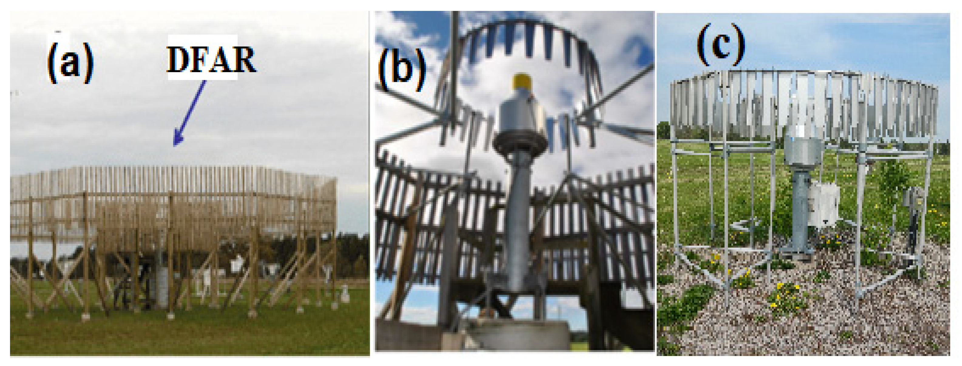
Figure 2.
Precipitation type represented by symbols (C = clear, snow, S = snow, SP = snow pellets , IP = ice pellets, snow grain = SG, IC= ice crystal, R=rain , L = Drizzle, P= unknown, M = mixed phase, ZL = freezing drizzle, and ZR= freezing rain, (a), temperature (b), and 10 min averaged wind speed ( and 1 min averaged maximum wind measured at 3 m height.
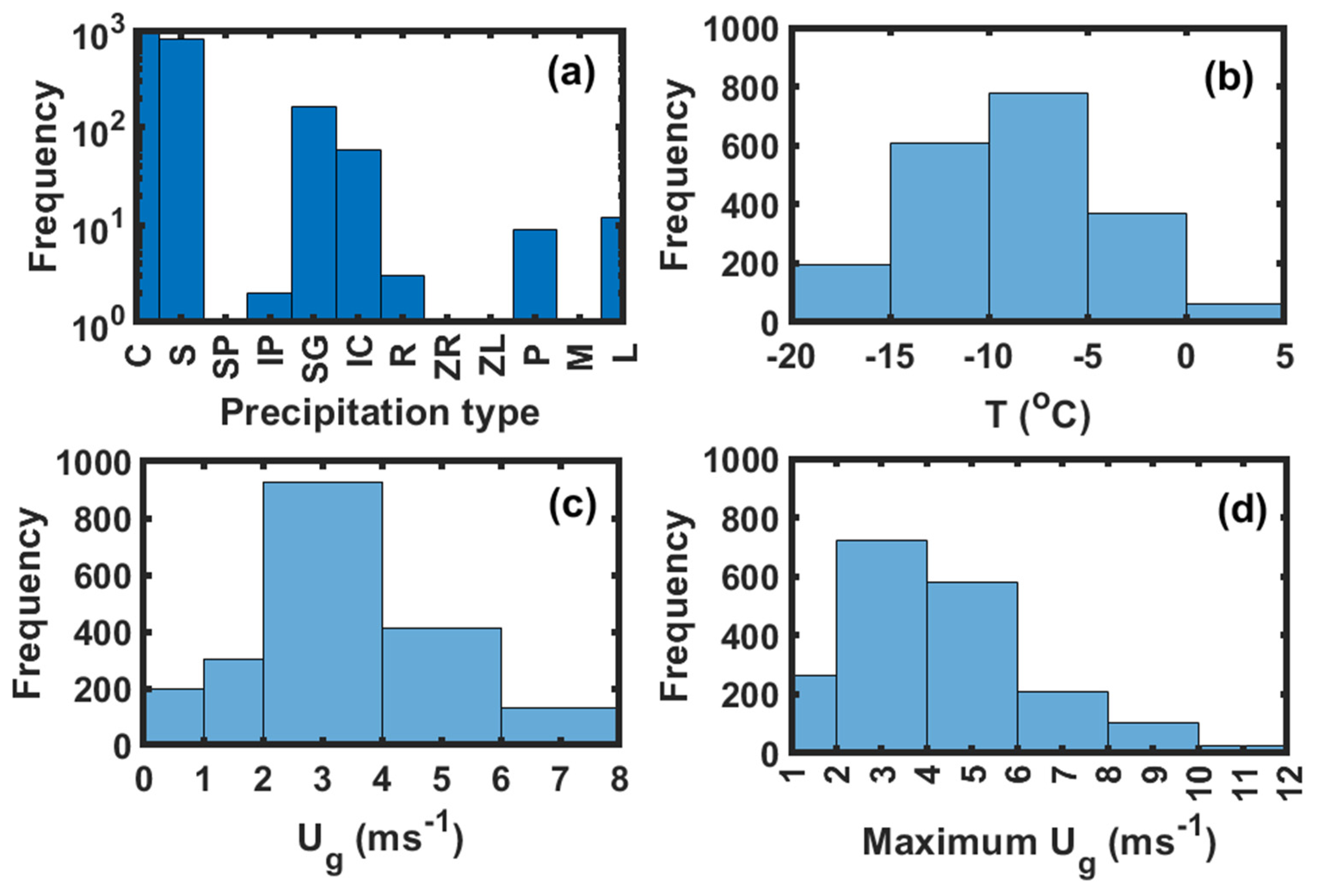
Figure 3.
The frequency distribution of fall velocity () of snow (a), snow grain (b), ice crystals (c) and drizzle (d) based on the PARSIVEL2 data.
Figure 3.
The frequency distribution of fall velocity () of snow (a), snow grain (b), ice crystals (c) and drizzle (d) based on the PARSIVEL2 data.
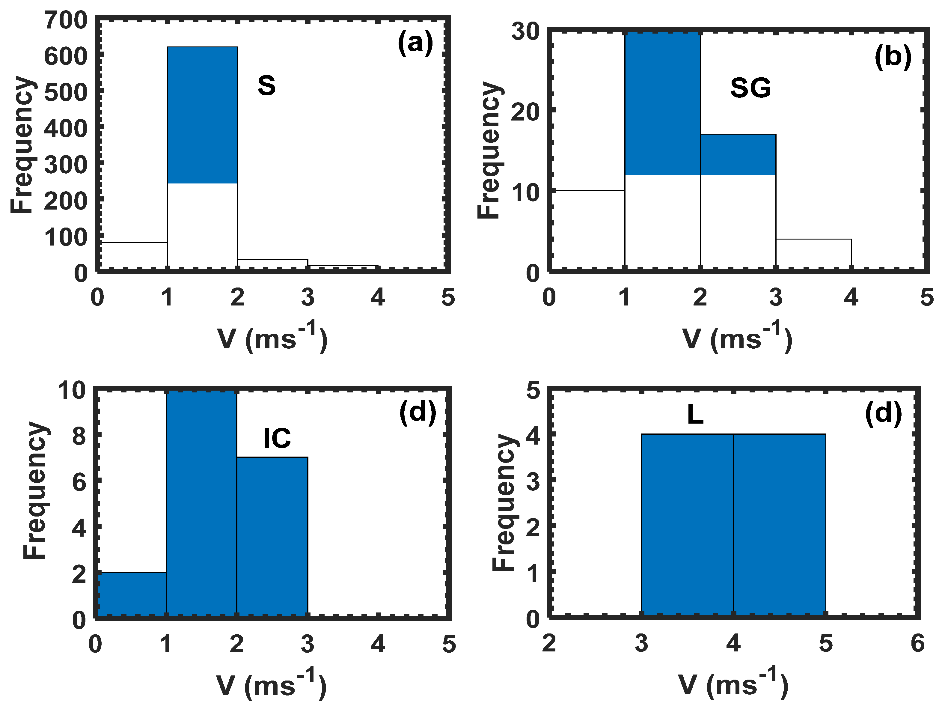
Figure 4.
Collection efficiency (CE) of Geonor with double Alter shield as a function of gauge height wind speed () and fall velocity (V) (a), comparisons of the parameterization of CE as a function of (b), Rasmussen et al., 2012 (Rass12) and as a function of and (d) against observation.
Figure 4.
Collection efficiency (CE) of Geonor with double Alter shield as a function of gauge height wind speed () and fall velocity (V) (a), comparisons of the parameterization of CE as a function of (b), Rasmussen et al., 2012 (Rass12) and as a function of and (d) against observation.
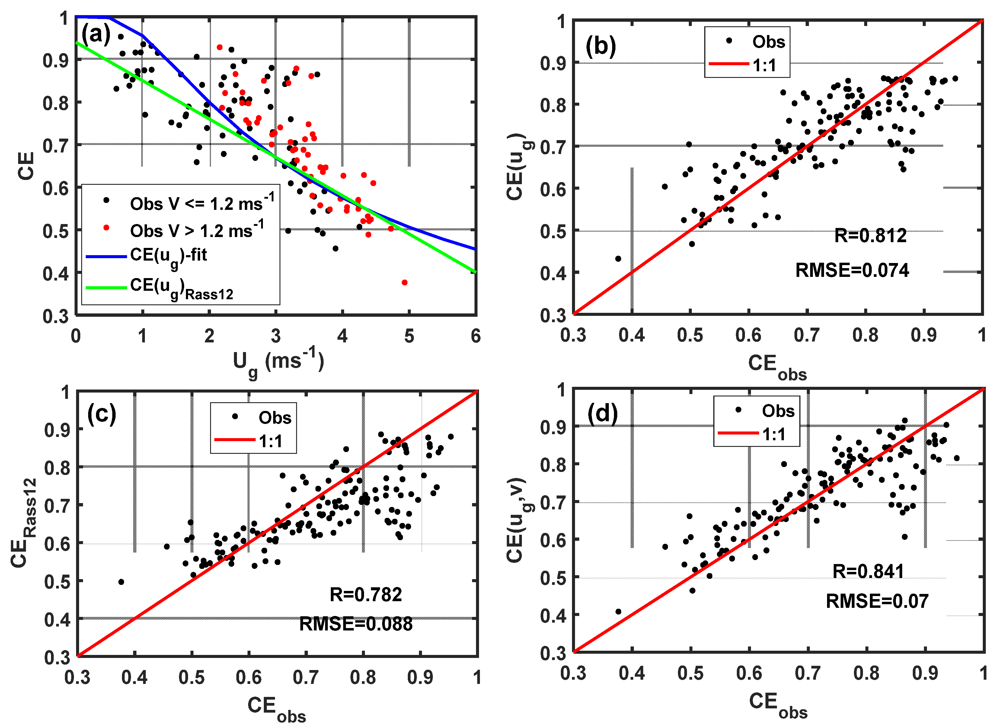
Figure 5.
Collection efficiency of HotPlate (a), FD12P (b), and PARSIVEL2 (c) as a function of wind speed () measured at gauge height level (c).
Figure 5.
Collection efficiency of HotPlate (a), FD12P (b), and PARSIVEL2 (c) as a function of wind speed () measured at gauge height level (c).
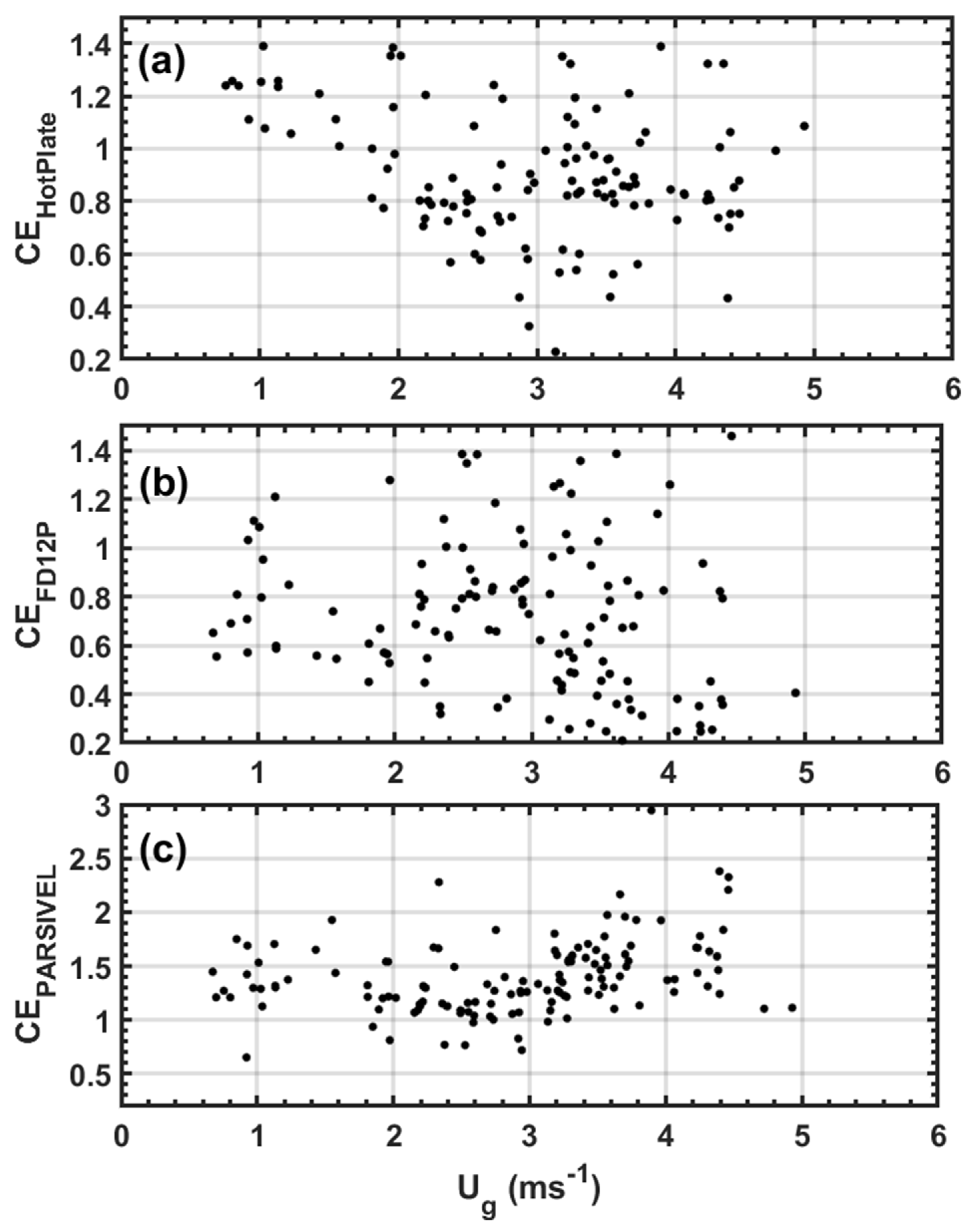
Figure 6.
Comparisons of the solid precipitation and PARSIVEL2 (a), HotPlate (b), and FD12P (c).
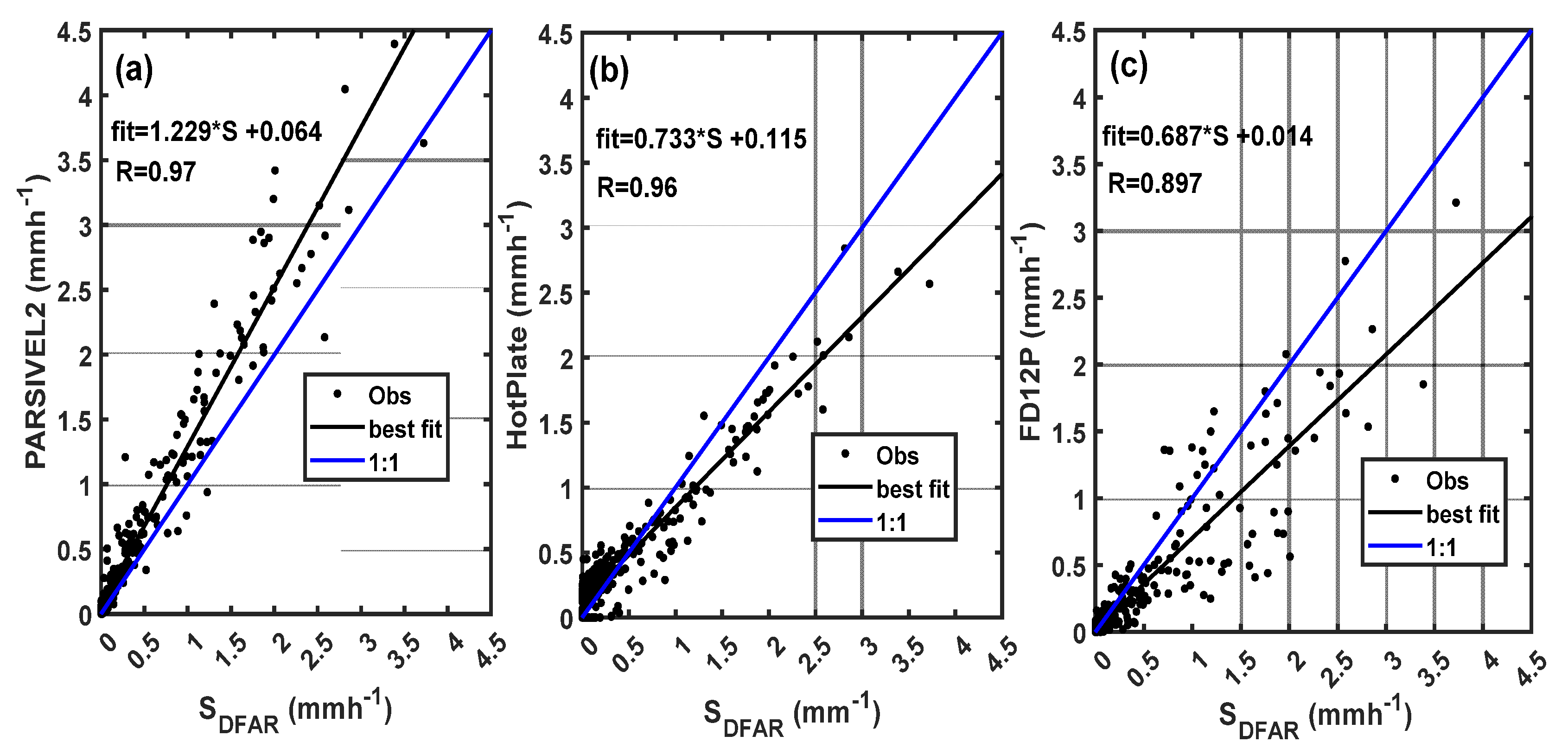
Figure 7.
Comparisons of snow accumulation of SDFAR, and several instruments given in Figure 6, unadjusted (), adjusted (adj) based on the transfer functions in Table 1 (), (), and ) (a) and the associated solid precipitation intensities (b).
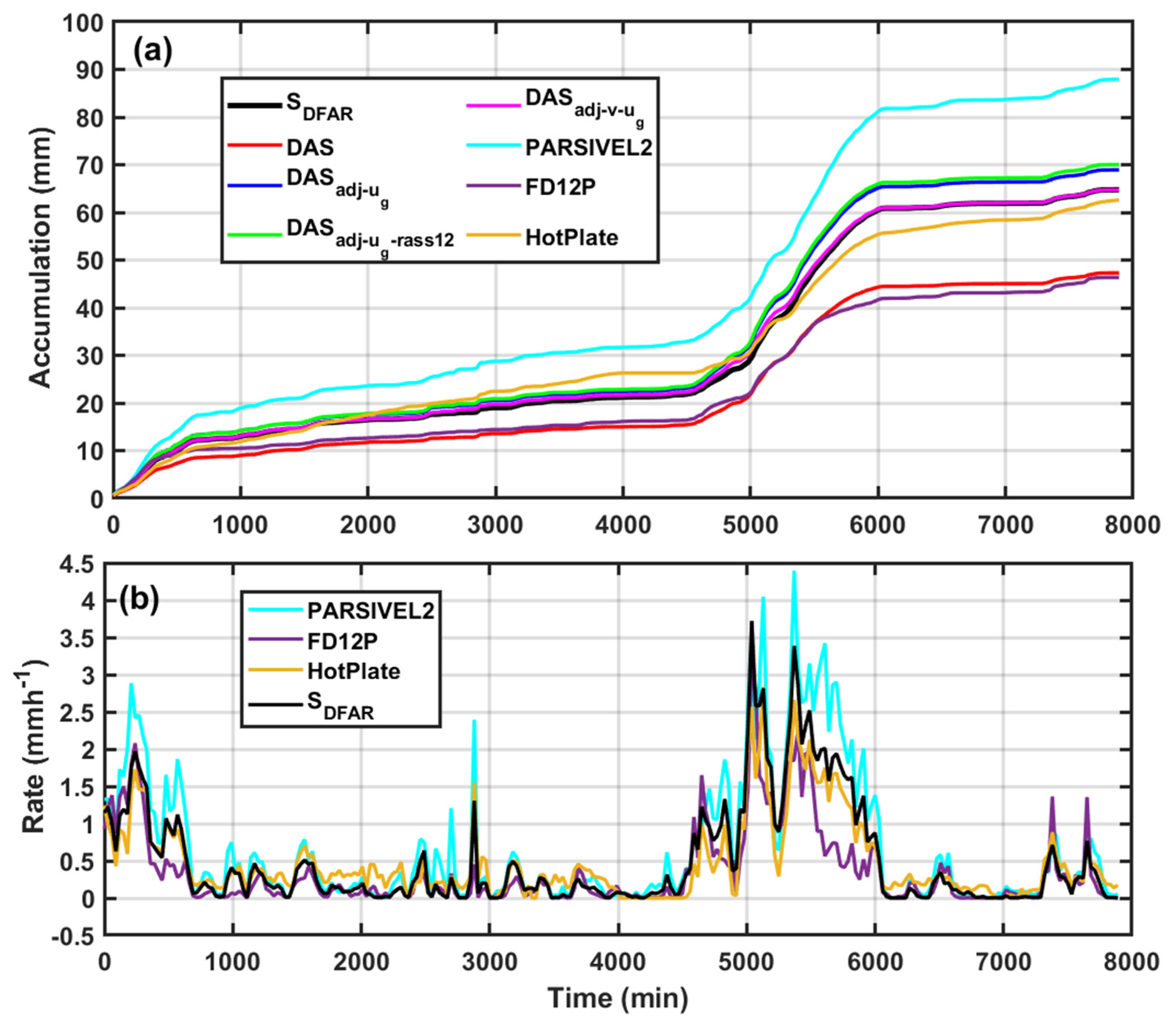
Figure 8.
Collection efficiency of Pluvio2 with a single Alter shield ( ) (a), the observed ( compared to (b), , (Boudala et al., 2017) (c) and (Kochendorfer et al., 2017) (d).
Figure 8.
Collection efficiency of Pluvio2 with a single Alter shield ( ) (a), the observed ( compared to (b), , (Boudala et al., 2017) (c) and (Kochendorfer et al., 2017) (d).
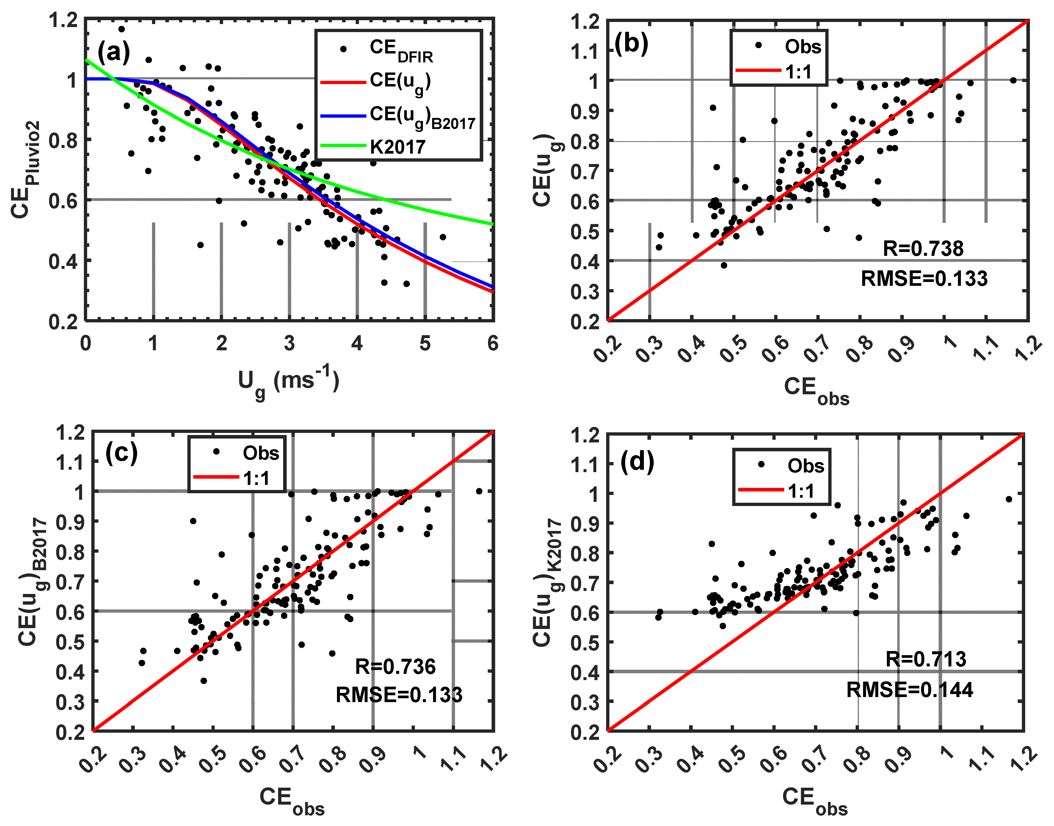
Figure 9.
Accumulation of S based on the , adjusted (adj) with (), (), and (.
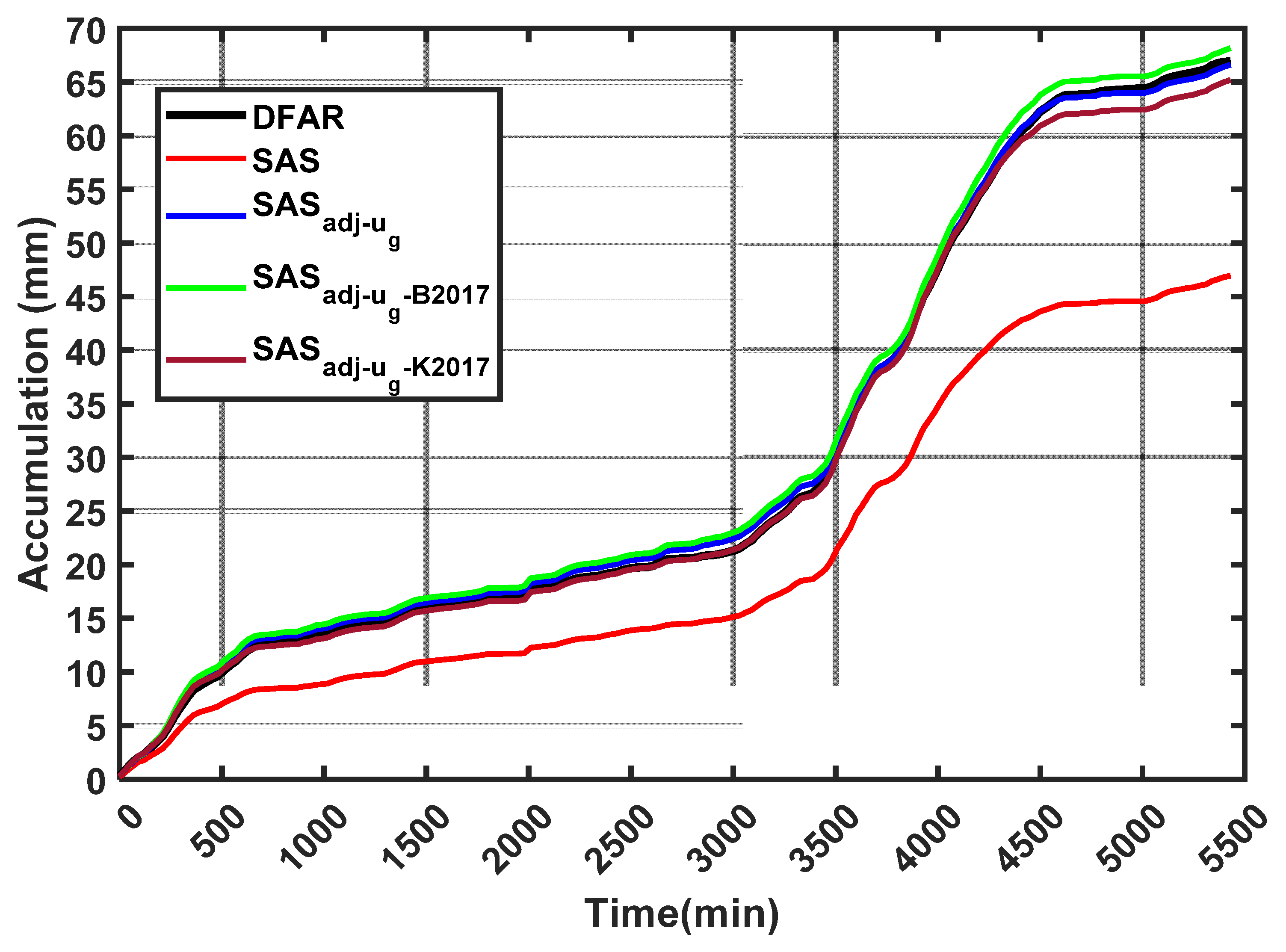
Figure 10.
Comparisons of visibility measured using the FD12P () and a number of parameterizations in Table 2 of (a), the best fit lines (b) and (c), and based on Boudala and Isaac, (2009) (d). Water equivalent solid precipitation intensity thresholds very light (VLT), light (LT), moderate (MOD), and heavy (HEAV) based on visibility adapted by Transport Canada are shown including the calculated Mean Absolute Error (MAE), Mean Difference (MD), and Standard Deviation of the Difference (STDD).
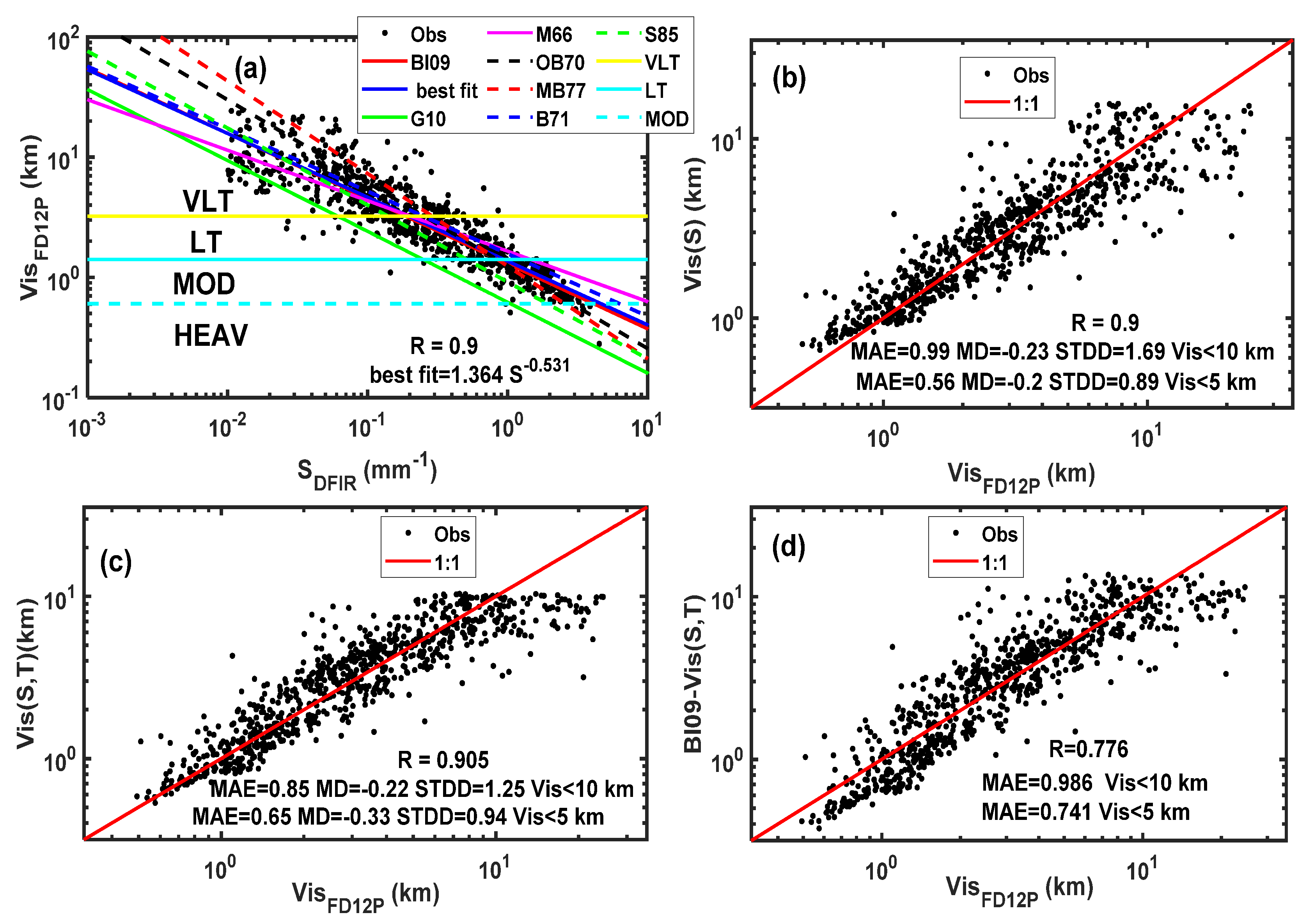

Table 1.
Transfer functions for collection efficiency (of) double Alter Geonor gauge.
| Sources | Catch efficiency parameterization | RMSE |
| In this work-Geonor double Alter shield | 0.074 | |
| In this work | 0.07 | |
| Rasmussen et al., 2012 | 0.09 |
Table 2.
Transfer functions for collection efficiency (CE) for single Alter shield Pluvio2.
| Sources | Catch efficiency parameterization | RMSE |
| In this work | 0.13 | |
| Boudala et al., (2017) | 0.13 | |
| Kochendorfer et al., (2017) | 0.14 |
Table 3.
Visibility parameterizations based on solid precipitation.
| The source | The parameterizations |
| This work -Vis(S) | ) |
| Boudala and Isaac, 2009 (BI09(S)) | |
| This work -Vis(S,T) | |
| Boudala and Isaac, 2009 (BI09(S,T) | |
| Mellor (1966) (M66) | |
| Warner and Gunn (1969) | |
| O’Brien (1970) (OB70) | |
| Gultepe et al. (2010) (G10) | |
| Stallabrass (1985) (S85) | |
| Fujiyoshi et al. (1983) | |
| Bisyarin et al. (1971) (B71) | |
| Muench and Brown (1977) (MB77) |
Disclaimer/Publisher’s Note: The statements, opinions and data contained in all publications are solely those of the individual author(s) and contributor(s) and not of MDPI and/or the editor(s). MDPI and/or the editor(s) disclaim responsibility for any injury to people or property resulting from any ideas, methods, instructions or products referred to in the content. |
© 2023 by the authors. Licensee MDPI, Basel, Switzerland. This article is an open access article distributed under the terms and conditions of the Creative Commons Attribution (CC BY) license (http://creativecommons.org/licenses/by/4.0/).
Copyright: This open access article is published under a Creative Commons CC BY 4.0 license, which permit the free download, distribution, and reuse, provided that the author and preprint are cited in any reuse.


