1. Introduction
Power distribution has become more efficient and reliable with the advent of smart grid. Although the distribution and supply services have been unbundled in recent years at most restructured electricity markets in smart grid systems. Having unbundled, load balancing, load forecasting and demand response management using smart meters continue to pose significant challenges to industry and research. Since the rate of power or electricity supply to customers has become competitive that needs to be tailored to the customer’s behavior based on accurate information from electricity suppliers. To do so, a deep knowledge of the customers’ behavior is required for the electricity provider not only for ensuring the uninterrupted quality of electricity but also for customer satisfaction. Again, for the sake of tariff planning, the customers’ contributions to the entire daily load pattern are gaining increased attention. Yet identifying and classifying customers effectively is very challenging. This paper elicits a general schema for analyzing electrical load supposedly used to produce effective results [
1].
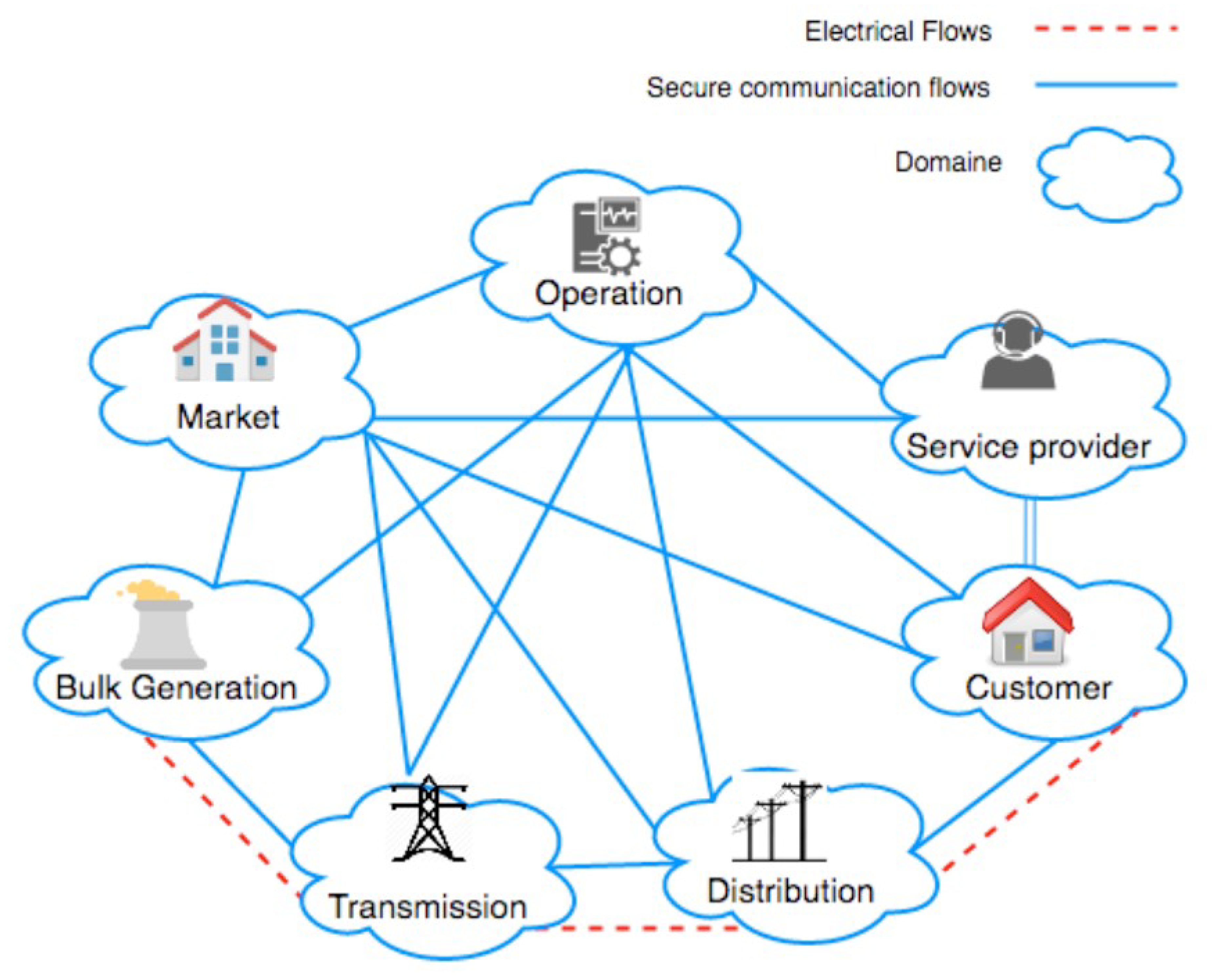
The basic model of a smart grid system is depicted in
Figure 1, the interconnection of dependent domains used for power generation, transmission, distribution, market, operation, and customers as well [
2].
The relevant consumption pattern for categorizing customers is likely to establish a suitable customer decision model on the basis of load pattern behavior.
An efficient clustering technique has been proposed in this study that employs the raw meter data collected daily from smart meter with an aim to load profiling, using clustering as well as the K-means algorithm. In doing so, the machine learning algorithm is used to time series data generated from the smart meter. This data source provides utilities with information that can be used to develop customized electricity load profiles (PCs) as well as to aid in areas such as improved load forecasting; Demand Side Management (DSM) strategies, Time of Use (ToU) tariff design and electricity settlement. Knowing the form of the power consumption might be helpful for deciding how to manage local energy generation and consumption for planning and operating energy systems. There is growing concerned about the type of electricity utilized as a result of the accessibility of cutting-edge load control technology and the expanding variety of flexible demand management options that provide incentives and rewards to the participating customers. Conceptually, electricity customers could be categorized based on their consumption. However, the following challenges are associated with the analysis of load profiling:
Vague interpretation: The load patterns of customers who engage in the same activity or who use the same commercial code may differ significantly.
Efficiency: Therefore, utilizing classification based on the type of activity and commercial codes to represent the precise characteristics of power demand is ineffective.
Macro categorization: The ability to differentiate between a small number of macro categories (such as residential, commercial, industrial, or other niche categories like electric lighting and traction) is restricted.
This paper focuses on the characteristics and habits of consumers and cites pertinent works in its discussion of these topics. The topic of evaluating the efficacy of clustering algorithms for classifying load patterns was then discussed in detail. The contracted power, supply voltage level, annual active and reactive energy (maximum, minimum, average value, and standard deviation), utilization level (defined as the energy consumption to rated power ratio), and power factor are a few examples of these external features. The usage of macro-categories, when applied to all electrical users, minimizes the number of load patterns that must be handled concurrently by the categorization methods inside each macro-category, leading to more cost-effective computation procedures.
The analysis involves two-fold steps as follows:
The categorization process’ main step is to group load patterns using the appropriate clustering approaches. Each clustering technique can be executed by configuring the necessary parameters. In certain clustering techniques, the results depend on the initialization of the centroid.
Based on the clustering techniques load distribution among varied customers will be narrowed down to a number of specific customers. Five categories of electric consumers are the targeted class from the sample dataset that will be followed by the relevant machine learning technique either supervised or unsupervised.
2. Related Works
A sheer number of authors have already examined the load profile of providing services beyond billing using fine-grained data on electricity consumption. A lot of research has been done on non-intrusive load monitoring (NILM), which tries to figure out how much energy each appliance in a home uses. This NILM method uses measurements of power use taken at high frequencies, usually between 1 Hz and multiple times per second, and does not require the installation of extra sensors [
1,
4]. In order to deliver unique services, such as feedback to encourage more energy-efficient behavior among users, it is necessary to have the ability able to assign each appliance its true proportion of electricity consumption [
2]. The accuracy of NILM techniques suffers in real-time contexts due to the lack of high-frequency measurements and the need for time- and data-intensive training operations [
5]. In contrast to NILM methods, our focus is not on calculating the consumption of specific appliances but rather on identifying broad categories of end users. Also, we don’t need data sampled very frequently, as we may make do with data taken once an hour or even less frequently. Electricity consumption data was normally recorded at 15-, 30-, or 60-minute intervals, although a number of related methods relied on this data. Such data have even been used by a number of authors to examine how consumption patterns have changed over time [
2,
6,
7]. Again in [
8] Geoffrey et al. proposed a predictive model comparing the analysis of energy consumption among regression, decision tree, and neural networks. These frameworks aim to forecast future electricity consumption on the customer side and, by connecting these patterns across time, to support supply management on the electrical provider side [
9]. According to [
10], where 471 consumers were tracked down and inspected by the power company to do automatic clustering, this is a noteworthy example of the clustering techniques for grouping electrical load patterns. The authors find instances of wasteful billing methods throughout their analysis of the cluster results and current non-residential customer rates (for instance, when there is a weak association between discriminatory variables and real load patterns). Nishant et al. in [
11] addressed an ANN model for accurate load forecasting to resolve the challenges imposed by conventional methods like mean and mode.The suggested methods concentrate on finding patterns in the available consumption statistics rather than tying them to particular traits of the family or commercial structure that caused the patterns to develop. Additionally, the conclusions from that approach are based on modest data sets that include traces from about 3000 households. In our research, we take into account consumption traces from more than 8760 hours of data) for a group of 24 representative facilities with a range of end-use levels. By utilizing self-organizing maps, Kushan et al. are able to discover new(commercial) consumers as well as consumption patterns that differ from "typical" behavior. There are a variety of other comparable techniques that use self-organizing maps (SOMs) to evaluate data sets that contain traces about numerous different customers[
12]. A neural network-based unsupervised learning technique that can be used to automatically identify clusters from an otherwise unstructured (and unlabeled) set of data is the core of SOM. An hourly load data for a Set of 24 Facilities from residential, commercial, industrial, and various end-users has been calculated in [
13]. To detect the anomalies in the power consumption in the smart grid, recognizing the load pattern is highly important [
14]. However, various risks are associated while considering the smart meter data [
15]. The wide ranges of cyber attacks [
16] are liable to make any disruption to the meter data that might cause radical changes in load usage. Several machine learning algorithms such as classification, clustering, neural networks, and data mining are state-of-the-art techniques that can be applied to implement the precise load classification[
17,
18].
3. Data acquisition and preparation
Load profiling in the big data era requires processing large amounts of data. With the proliferation of Advanced Metering Infrastructure (AMI) devices, through load profiling more information can be collected from the power consumption data of individual customers via the smart meter. Load profiling enhances our knowledge of electrical consumption patterns. This analysis performed load profiling among several ranges of electric users based on data from smart meters in order to understand the variance in load profiles at different time intervals.
3.1. Data Acquisition
The daily collection of consumer data from smart meters is necessary for the research and design of a reliable clustering model. In this paper, we collect the smart meter data from the Mendeley dataset [
13]. The dataset is based on Hourly Load Profile Data collected from smart meters from diverse types of consumers ranging from households to industries under the hub of the smart grid. This dataset comprises of load data for 24 hours of power usage at an hourly interval from various end-users, including industrial, commercial, and residential consumers, over an entire year (8760 hours of data). The dataset includes 18 simulated buildings that were climate-adapted to New Jersey using the physics-based building simulator, an Energy Plus-based tool that captures the functions of the buildings, as well as load data from six reference buildings from publicly available Energy Plus reference buildings. In single- and multi-node energy systems, such as nano grids, microgrids, or integrated systems in distribution networks, where each building’s load profile corresponds to its electricity usage, a dataset can be used to represent the systems. This dataset supports a wide range of engineering, economic, and environmental assessments by assisting researchers and practitioners globally in modeling their defined/modified test systems. As a starting point in the typical load patterns for a given loading state, the categorization information for each client is provided in a way that creates load patterns with comparable forms. Following are the two attributes of this dataset to be used throughout our analysis:
the power measurement in [kW], referred as the peak value of the typical daily load pattern;
the normalized representation of load pattern in (RLP), computed by dividing the typical daily load pattern by its power rate.
3.2. Data Pre-processing
Customer behavior is measured through continuous metering or by setting up dedicated measurements based on daily load patterns. While considering M number of customers to monitor, e.g., through the application of statistics such as stratified sampling [
11], the data acquisition and preparation process can be summed up in three phases.
Phase 1-Pre-clustering is characterized by the following steps:
Data sampling preparation: The preparation of data sampling entails the choice of the time interval for the analysis (for conducting measurements), the rate of sampling (e.g., quarter-hour, half-an-hour, hour) and the careful checking of the technical specifications of the interval meters, in order to achieve acceptable precision for the measurement. The data collection amount is dependent on the amount of data storage available in the metering system, so there a compromise may be needed between a fast sampling rate and the duration of the observation period. Depending on the clustering method being used, the sample rate may change.
Bad data detection: Identifying days with faulty data in the load patterns, such as those caused by weather, power outages, and other irregularities. The performance of the Kohonen self-organizing maps (SOM) has been used for anomalous days identification. Bad data can be detected using several methods based on measurement results. Directly manipulating data on load power is possible, or the data from other sources can be used to generate additional information. A voltage magnitude monitor, for instance, can be very useful when detecting bad data, especially when there are short interruptions and voltage sags present.
Identification of the loading conditions: A statistical analysis of daily load patterns can be used to determine the load patterns (such as winter and summer seasons, with a possible inner divide into weekends, working days, Saturdays, and Sundays) for each time.
4. The clustering phase
Phase 2 includes the following steps:
Feature Selection For determining the representative load patterns for customer clustering purposes an appropriate set of features is selected; an easy selection could be based on the time-domain data on which the representative load pattern is developed. Then the feature extraction is performed on the selected features that lead to the clustering.
Feature Extraction The selected features are extracted as per the time series methods to obtain the desired attributes of the features associated with the dataset. This approach is done with the aim to make easing the following steps of machine learning.
Customer Clustering Using an appropriate machine learning technique, we could then divide our customers into K distinct classes.
Pattern recognition The pattern recognition is calculated for each of the K customer classes based on aggregated load patterns for the same customer class.
4.1. Feature Selection
The load data undergoes feature extraction once it has been pre-processed (bad data removed, samples taken, loading condition chosen). In this case, identical consumption patterns on the same day of the week were observed throughout the course of a month (e.g., all Mondays have a similar load profile, etc.).
The consumption profile of a day can be broken down into four distinct segments, each characterized by a distinct consumption pattern. These eras (each with 16 samples) were found to have relevant clustering features.
Time period 1: 6:00 am to 10:00 am.
Time period 2: 10:00 am to 2:00 pm.
Time period 3: 2:00 pm to 6:00 pm.
Time period 4: 6:00 pm to 10:00 pm.
Time-domain data: When all or some of the normalized power values are taken into account from the time domain measurements, it is easy to identify the characteristics of the mth representative load pattern, for m¼1, 2, y, M. In this way, you can get at a group of H direct form characteristics without having to resort to load pattern post-processing. As a result, the following equation describes the characteristics of the load patterns representation:
Thus, the following equation describes the set of characteristics that comprise the representation of load patterns.
whose m th component is represented by the vector
In this case, the number of H values can be chosen arbitrarily, up to the limit imposed by the meter resolution. In order to maximize the efficiency of data processing, a trade-off is made between accurately representing the pattern’s shape and using as few points as possible. The normalizing power P(m) is saved for each client segment separately.
4.2. Feature Extraction
This paper builds on and extends the related works [
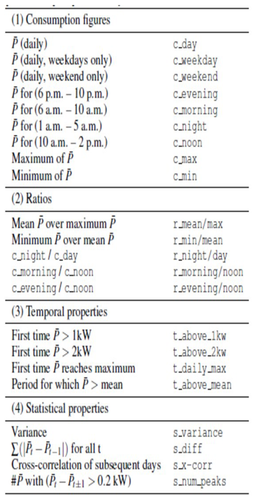
11] by defining a set of attributes that can be calculated using either daily consumption measurements or weekly/monthly/yearly averages of consumption. Consumption pattern, ratios, temporal properties, and statistical properties are the four classes of features identified. The spending habits are consistent with elementary summaries of what a typical family spends on consumables. Examples of consumption patterns include the lowest and highest consumption numbers on a given day, as well as the daily and hourly averages for certain times of day (such as early morning and late night). Whereas ratios denote the fractions of daily consumption averages at various times. For instance, we look at how much on average people consume between breakfast and lunch. Furthermore, the temporal attributes specify what time of day specific occurrences take place. There are several examples that serve as illustrations, though, including the daily consumption peak and the time of day that a certain consumption threshold is first reached. In the third stage, the consumption curve’s qualitative characteristics are captured using statistical properties. The cross-correlation between these profiles is then calculated to find the correlation between consumption profiles (within the same household) on different days. Table 2 lists all of the characteristics of the time domain that have been defined in the context of the implementation. The right column indicates the time intervals from morning to noon, then respectively to evening, and night as the time periods from 6 a.m. to 10 a.m., 10 a.m. to 2 p.m., 2 p.m. to 6 p.m., and 6 p.m. to 10 p.m., as denoted the various characteristics of the time domain.
Table 1.
Feature selection and extraction.
Table 1.
Feature selection and extraction.
4.3. Clustering Techniques for Load Profiling
Clustering is a technique to identify patterns in data and is useful for exploratory data analysis, anomaly detection, customer segmentation, and pattern recognition (here load profiles). It works as a powerful tool to reveal insights that may not be addressed through other methods of analysis to understand data and this can help load profiling by comparing the customers’ load usage behavior. These behaviors are all included in the same cluster despite having the highest intra-cluster and lowest inter-cluster similarity. It indicates how few clusters are used to aggregate comparable load profiles.
Our next step is unsupervised training, where the networks are taught to form their own rules. In order to accomplish this, we must assume that input patterns sharing common features are class members and that the network will be able to identify those characteristics across the range of input patterns. Due to the nature of competitive learning, only a single neuron in the network’s output is active at any given moment, making unsupervised systems based on it potentially very intriguing. Neurons that are activated in this way are referred to as winning neurons or simply winning neurons. Neurons that are activated in this way are referred to as winning neurons or simply winning neurons.
The self-organization process involves four major components as follows step-by-step:
Initialization: The connection weights are all initialized with small random values.
Competition: The neurons calculate their respective discriminant functions based on each input pattern. The neuron with the smallest discriminant function is declared the winner.
Cooperation: Using the winning neuron, the topological placement of neighboring neurons is determined, providing a basis for cooperative behavior.
Adaptation: Through appropriate adjustment of the associated connection weights, the excited neurons decrease their individual values of the discriminant function in relationship to the input pattern, thereby increasing the response of the winning neuron to a subsequent application of the same input pattern.
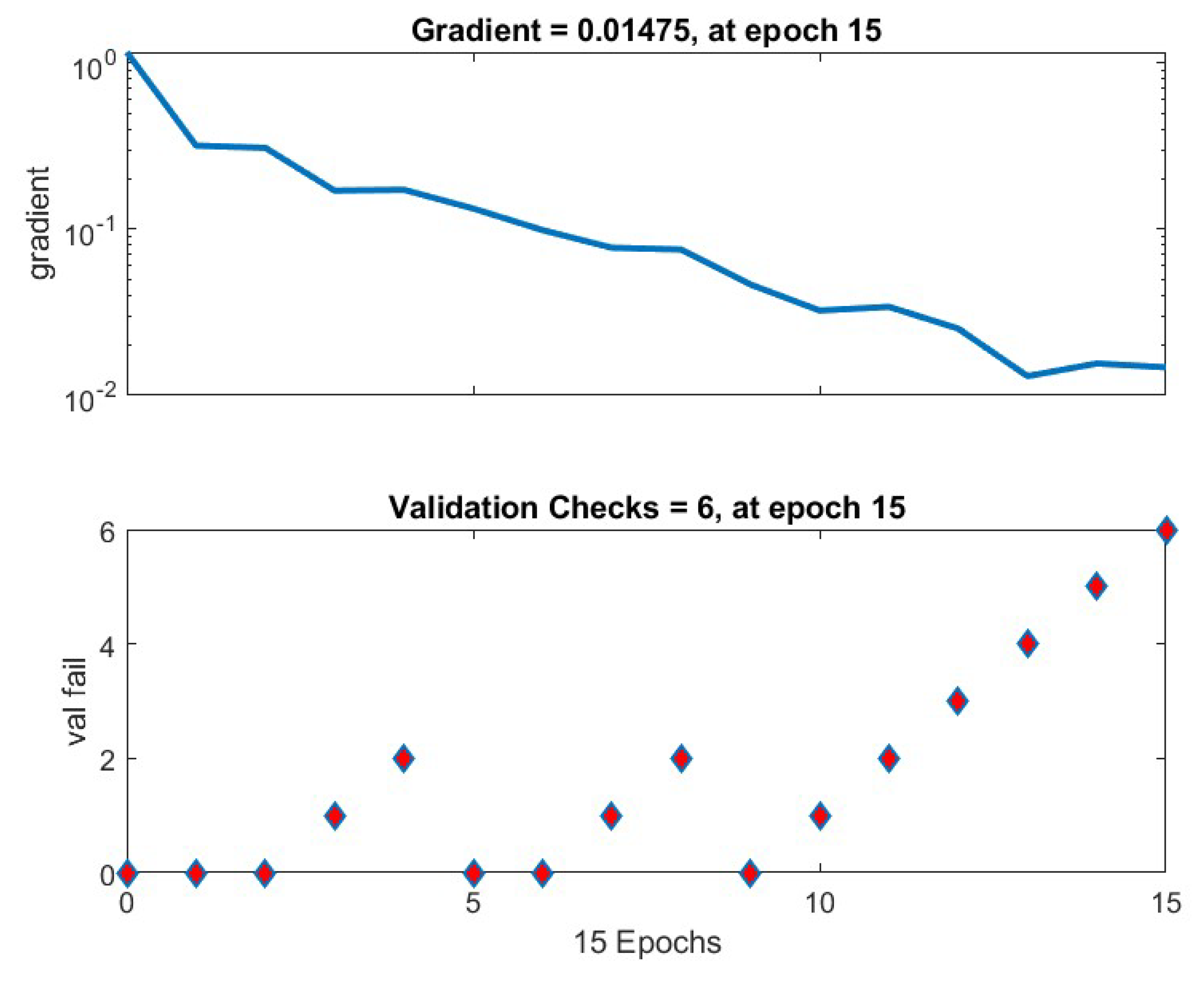
The Training State shows the number of Epoch=15 with Gradient 0.01475 and checks with validation 6.
Figure 2.
Training State Plot.
Figure 2.
Training State Plot.
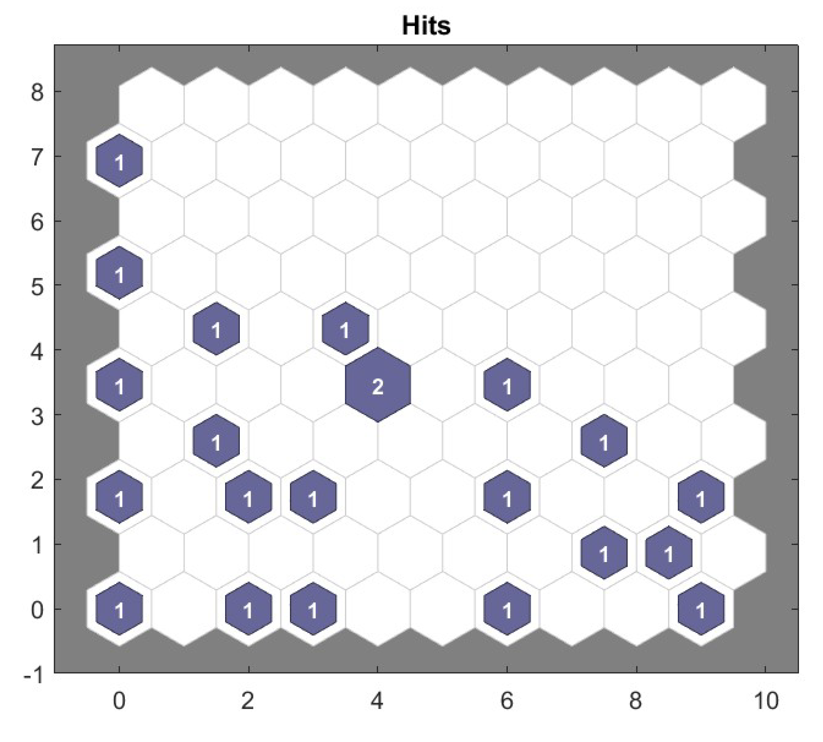
For the clustering in the neural network, the 98 samples are fed into the network of 14 inputs and resulted in 5 classes. Here the 14X22 self-organizing map(SOM) hits plot interprets, as it has grouped 14 inputs into 5 different classes.
Figure 3.
Clustering Hit Plots.
Figure 3.
Clustering Hit Plots.
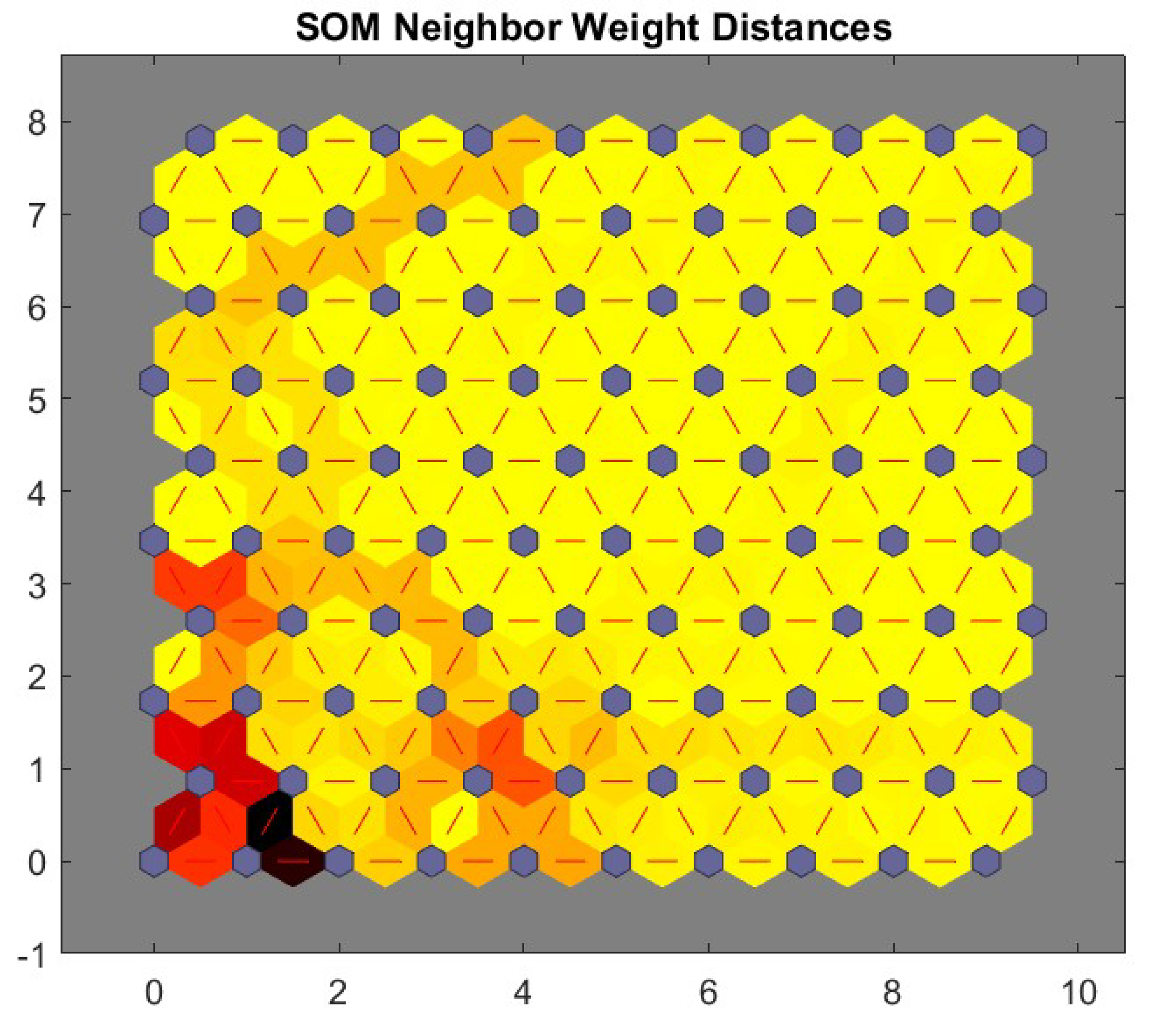
Figure 4.
SOM Neighbor Weight Distance.
Figure 4.
SOM Neighbor Weight Distance.
5. Evaluation
Having determined the bounds clustering and unsupervised learning steps we then present the results of our comprehensive analysis of the load data and quantify the error introduced by the model.
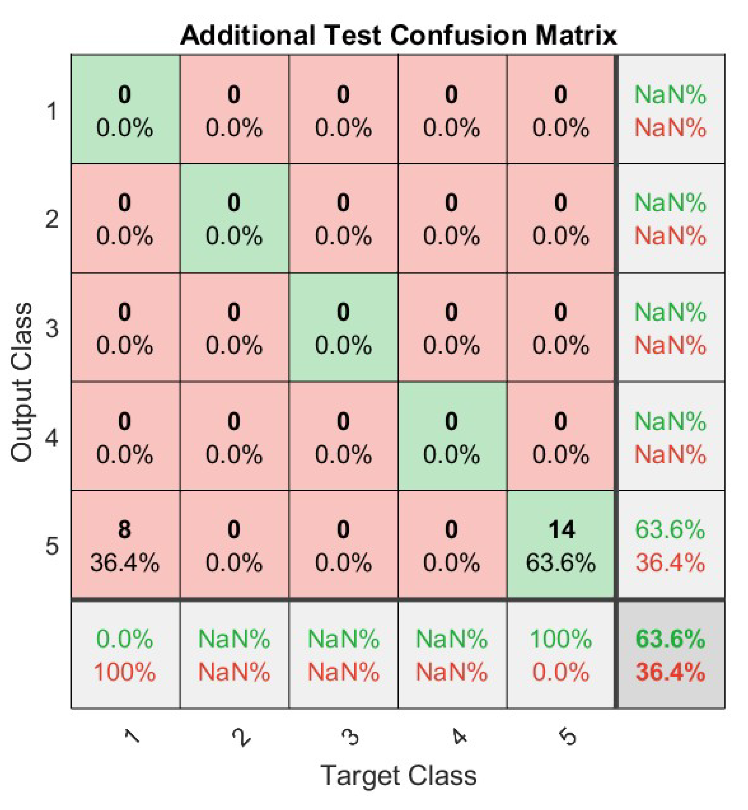
Figure 5.
Confusion Test Matrix.
Figure 5.
Confusion Test Matrix.
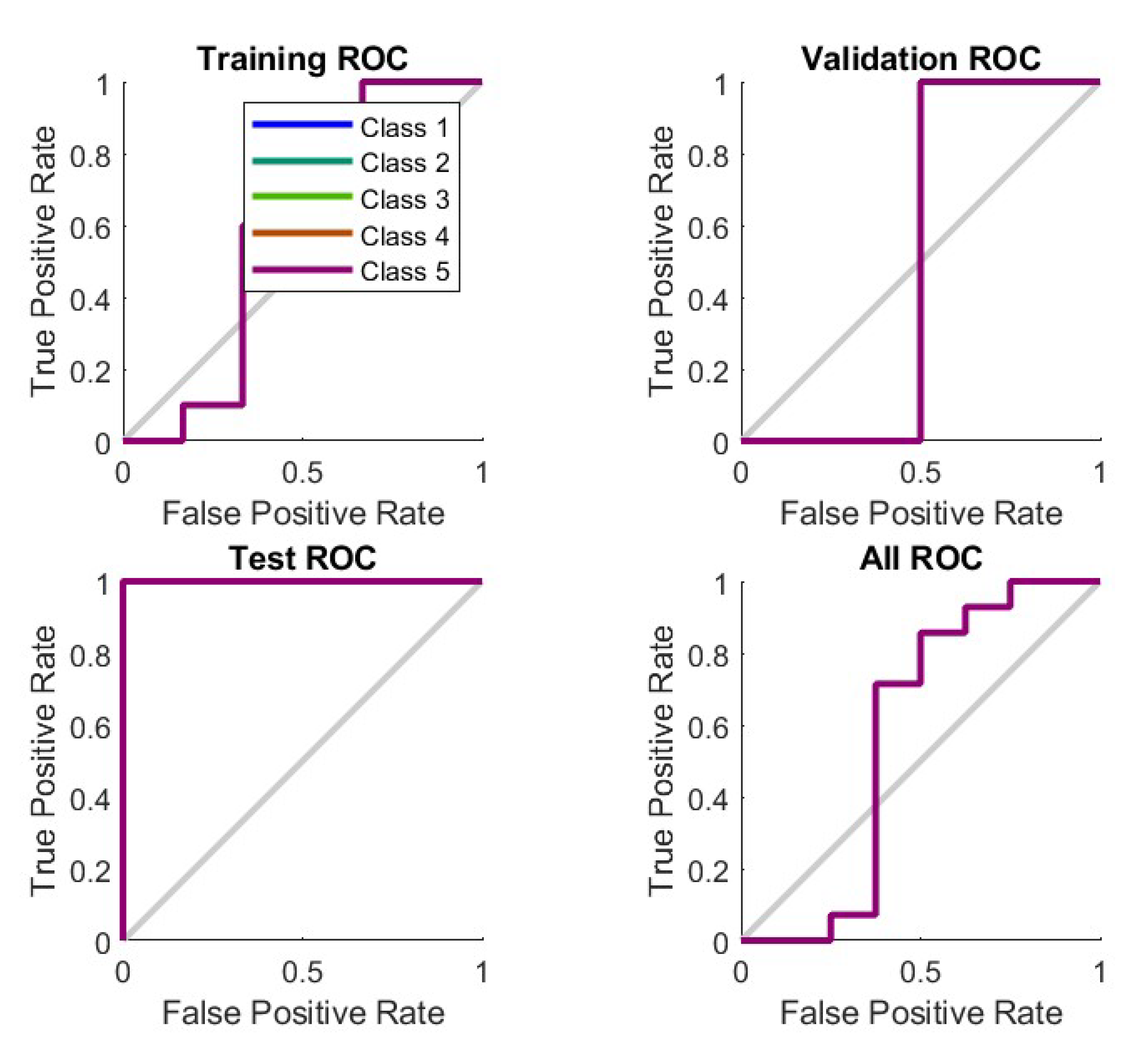
Figure 1 shows how clients were categorized by time slot. One property is the maximum single value and the other four are the maximum electrical load. The raw dataset was reduced from 2,53,760 samples to 35,600 samples, with the most informative load profile clustering information preserved by the feature matrix. These load profiles were clustered using SOM. The total of each point’s distance to the centroid for all 5 groups is reduced iteratively by this clustering method. Most machine learning models for binary classification do not simply generate a value of 1 or 0 while making a prediction. Instead, they produce a continuous number in the [0,1] range. Values that are at or above a given threshold (for example, 0.5) are classed as 1, whereas those that are below the threshold are classified as 0. The points on the ROC curve represent the FPR and TPR for various threshold values. Classifications will change depending on the specified threshold value, which can range from 0 to 1. The "up and to the left" orientation of the ROC curve indicates superior performance when classifying the efficacy of a model.
Figure 6.
Cluster weight.
Figure 6.
Cluster weight.
5.1. Results and Discussions
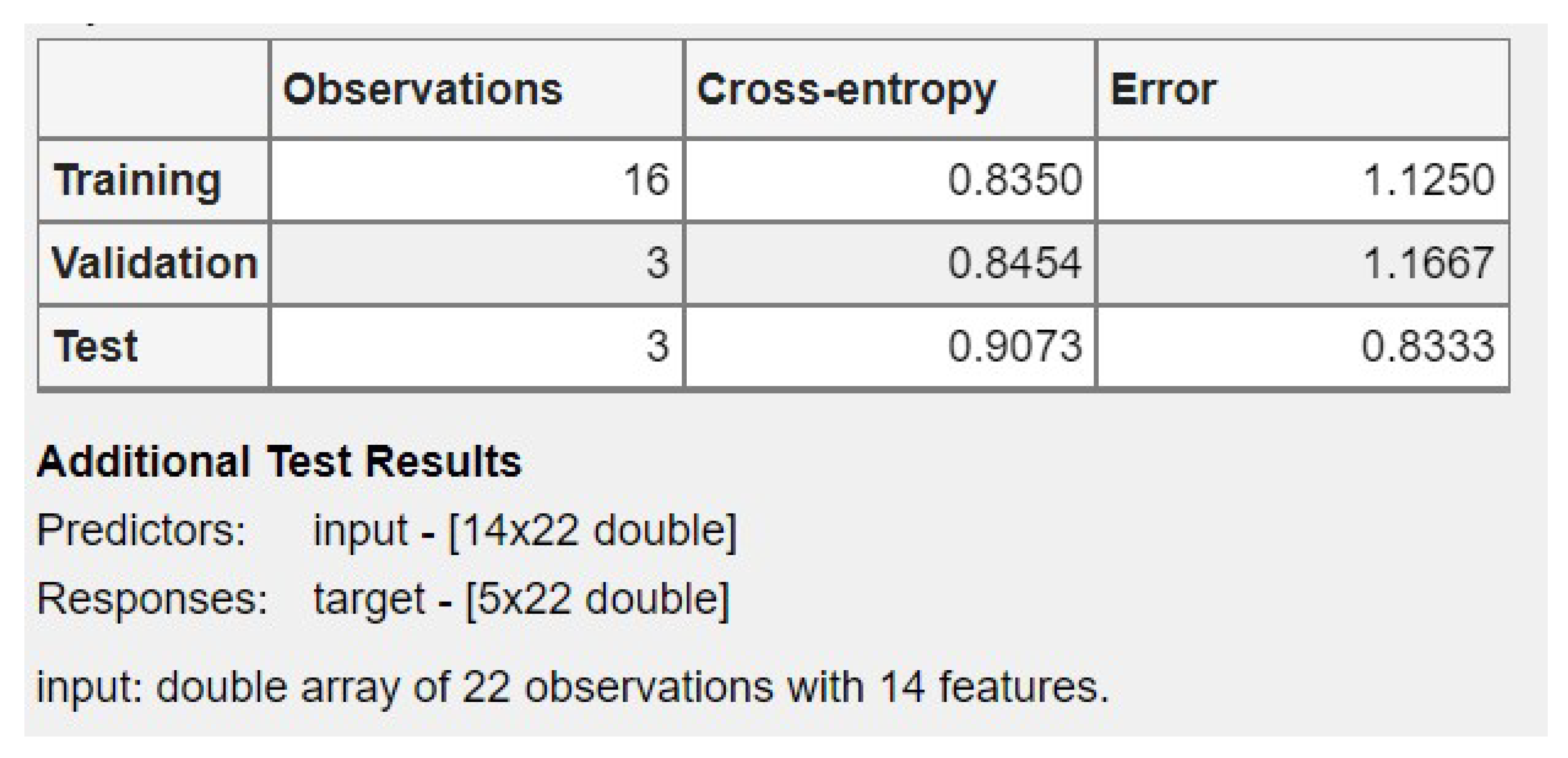
The application of load profiling to demand response differs due to the variety of demand response algorithms. Various researchers have looked at the subject from various angles. It’s easy to understand how load-based approaches are typically expressed as optimization problems with multiple object functions and constraints. The training results show an error rate of 1.12% for training samples, 1.1667% for validation checking as well as 0.833% for testing another set of sample data with the trained data in the neural network pattern recognition technique.
Methods and standards for evaluating demand response. Because of the pervasiveness of AMI technology, load profiling may glean a variety of information from the electricity usage statistics of individual users. Here from the smart meter reading data of various customers the maximum load consumption rate per half an hour of a selected date has been taken into consideration to carry on the machine learning training approach. Then with the aforementioned learning algorithm, the SOM has resulted from the clusters of 5 customers along with their load pattern usage of the particular date. This proposed mechanism is able to predict the load pattern behavior for a week or even a month which can successfully be analyzed for not only demand and supply but also for anomaly detection in the load calculation. The five classes of customers are categorized from the dataset after applying the machine learning techniques such as households, educational institutes, industries, commercial, and hospitals.
Figure 7.
Training Results.
Figure 7.
Training Results.
The consumer load profiles are often projected in peak analysis. However, a probabilistic analysis of irregular peaks was not taken into consideration. The peak analysis of load usage among the customers may be represented as a trade-off in time and power measure in kW. Here the variable regulates the allowable tolerance for irregular peak analysis.
Figure 8.
Load Pattern Behavior.
Figure 8.
Load Pattern Behavior.
For instance, the assignment of
as 1.5 represents 50% tolerance for irregular peak detection.
Figure 9. The regular peak analysis for a consumer over 1 day; where LP and IP stand for load profile and irregular peak with 50% tolerance (1.5
< 2) and irregular peak with 100% tolerance (
> 2) are shown to depict the peak analysis. The knowledge of peak analysis can be very helpful for utilities to reduce uncertainty in load forecasting and aggregated load management. Peak analysis is very effective in showing the probability of occurring irregular peaks of each consumer[
15]. In the proposed method, each consumer’s load profiles have been categorized using clustering, which can be defined as the ratio of time of a day’s regular peak for each customer.
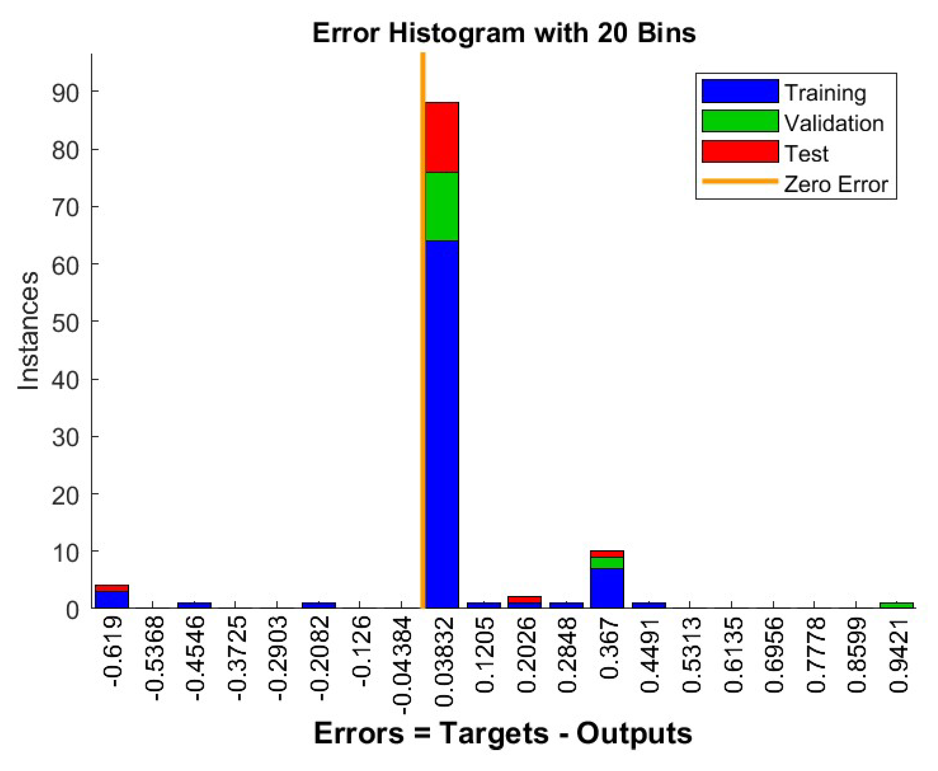
Figure 9.
Error Histogram.
Figure 9.
Error Histogram.
In terms of clustering algorithm formulation, the majority of The clustering approaches discussed are Euclidean in nature. metric. The results of these clustering approaches leave a lot to be desired. There’s still time to look into the pros and cons of using non-Euclidean metrics. Future research will focus on the possibility of non-Euclidean metrics. The current and future structures of energy systems include the data inherent in electrical load patterns has a huge impact. The term "categorization" refers to the process of developing and testing procedures. It is ideal for managing massive volumes of data gathered from a variety of the expanded smart metering technology as sources that is based on a large number of customers.
The details on clustering variants result in K=5 clusters. There is no uniform pattern of behavior among the numerous connection criteria for any of the clustering validity indicators investigated. The study performed here does not provide a definitive answer for the exponent of the Minkowski distance. Non-Euclidean metrics, on the other hand, produced superior results in some circumstances than Euclidean metrics.
6. Experimental Setup
Algorithm In this paper, we intend to implement machine learning algorithms on the Mendeley dataset of smart grid which is described in Section III. In the phase of Unsupervised training self-organizing map (SOM) is used. The comparison among classified results will be calculated by the error matrix afterward.
Tools In terms of tools, We have implemented our propounded model in MATLAB R2022a. The execution platform of both tools is on a Windows 10 PC with a configuration of an Intel Core i7 CPU (3.50GHz) and 64GB memory.
7. Conclusion and future work
In smart grid technology, load profiling techniques largely improve the understanding of electricity usage trends. This research presents an analytical evaluation of data mining strategies for load profiling with respect to clustering methods and criteria for evaluating clustering results. The information contained in load profiling has a lot of potential use both in academia and industries not for only research but also making proper energy plan for future. In this investigation, smart meters has been employed and machine learning to do in-depth analysis for load forecasting, demand response management, and event detection. The purpose of this research is to provide a framework for using and experimentally analyzing detailed information on power use collected by smart meters. In order to reduce computational cost, dimensional, and redundancy in data during clustering, 14 features were discovered in smart meter data. In the future, the application of load profiling in demand response event can be taken into consideration, where the feature can be divided into the incentive-based and price-based programs. In the framework of massive energy data analysis, we aim to extend our work to some significant load profiling obstacles and hurdles.
References
- G. Chicco, R. Napoli, F.P.P.P.M.S.C.T. Emergent electricity customer classification. Cognitive Computation. IEEE, 2005, Vol. 12.
- G Martín, A.; Fernández-Isabel, A.; Martín de Diego, I.; Beltrán, M. A survey for user behavior analysis based on machine learning techniques: current models and applications. Applied Intelligence 2021, 51, 6029–6055. [Google Scholar] [CrossRef]
- Gopstein, A.; Gopstein, A.; Nguyen, C.; Byrnett, D.S.; Worthington, K.; Villarreal, C. Framework and Roadmap for Smart Grid Interoperability Standards regional Roundtables Summary Report; US Department of Commerce, National Institute of Standards and Technology, 2020. [Google Scholar]
- Fang, X.; Misra, S.; Xue, G.; Yang, D. Smart grid—The new and improved power grid: A survey. Ieee 2011, 14, 944–980. [Google Scholar] [CrossRef]
- A clustering approach to domestic electricity load profile characterisation using smart metering data. Applied Energy 2015, 141, 190–199.
- Tso, G.K.; Yau, K.K. Predicting electricity energy consumption: A comparison of regression analysis, decision tree and neural networks. Energy 2007, 32, 1761–1768. [Google Scholar] [CrossRef]
- Ngai, E.; Xiu, L.; Chau, D. Application of data mining techniques in customer relationship management: A literature review and classification. Expert Systems with Applications 2009, 36, 2592–2602. [Google Scholar]
- Wang, Y.; Chen, Q.; Kang, C.; Zhang, M.; Wang, K.; Zhao, Y. Load profiling and its application to demand response: A review. Tsinghua Science and Technology 2015, 20, 117–129. [Google Scholar] [CrossRef]
- Jha, N.; Prashar, D.; Rashid, M.; Gupta, S.K.; Saket, R. Electricity load forecasting and feature extraction in smart grid using neural networks. Computers & Electrical Engineering 2021, 96, 107479. [Google Scholar] [CrossRef]
- Overview and performance assessment of the clustering methods for electrical load pattern grouping. Energy 2012, 42, 68–80, 8th World Energy System Conference, WESC 2010.
- Chicco, G.; Napoli, R.; Piglione, F.; Postolache, P.; Scutariu, M.; Toader, C. Load pattern-based classification of electricity customers. IEEE Transactions on Power Systems 2004, 19, 1232–1239. [Google Scholar] [CrossRef]
- Pitt, B.; Kirschen, D. Application of data mining techniques to load profiling. Proceedings of the 21st International Conference on Power Industry Computer Applications. Connecting Utilities. PICA 99. To the Millennium and Beyond (Cat. No.99CH36351), 1999, pp. 131–136. [CrossRef]
- Dataset on Hourly Load Profiles for a Set of 24 Facilities from Industrial, Commercial, and Residential End-use Sectors. [Online] Available: https://data.mendeley.com/datasets/rfnp2d3kjp/1., Accessed: 2020.
- Banik, S.; Saha, S.K.; Banik, T.; Hossain, S. Anomaly Detection Techniques in Smart Grid Systems: A Review. arXiv preprint arXiv:2306.02473 2023. arXiv:2306.02473 2023.
- Reinhardt, A.; Englert, F.; Christin, D. Averting the privacy risks of smart metering by local data preprocessing. Pervasive and Mobile Computing 2015, 16, 171–183. [Google Scholar] [CrossRef]
- Banik, S.; Banik, T.; Hossain, S.; Saha, S.K. Implementing Man-in-the-Middle Attack to Investigate Network Vulnerabilities in Smart Grid Test-bed. arXiv preprint arXiv:2306.00234 2023. arXiv:2306.00234 2023.
- Mohammad, A.T.; Mat, S.B.; Sulaiman, M.; Sopian, K.; Al-Abidi, A.A. Implementation and validation of an artificial neural network for predicting the performance of a liquid desiccant dehumidifier. Energy conversion and management 2013, 67, 240–250. [Google Scholar] [CrossRef]
- Pitt, B.; Kirschen, D. Application of data mining techniques to load profiling. Proceedings of the 21st International Conference on Power Industry Computer Applications. Connecting Utilities. PICA 99. To the Millennium and Beyond (Cat. No.99CH36351), 1999, pp. 131–136. [CrossRef]
|
Disclaimer/Publisher’s Note: The statements, opinions and data contained in all publications are solely those of the individual author(s) and contributor(s) and not of MDPI and/or the editor(s). MDPI and/or the editor(s) disclaim responsibility for any injury to people or property resulting from any ideas, methods, instructions or products referred to in the content. |
© 2023 by the authors. Licensee MDPI, Basel, Switzerland. This article is an open access article distributed under the terms and conditions of the Creative Commons Attribution (CC BY) license (http://creativecommons.org/licenses/by/4.0/).
