In this paper, we only consider simple and finite connected graphs, we refer to [1] and the references cited therein. Chemistry has been widely studied and applied in graph theory. The chemical compounds can be described in chemical graph theory, vertices represent the atoms and edges stand for the covalent bonds between atoms.

The molecular formula of a compound can represent different molecular structures and characteristics, but theoretical chemists are concerned about the physical and chemical properties of a compound and its relationship with the molecular formula of a compound. The topological index is considered as one of the most important methods to establish the relationship between molecular structure and its physicochemical properties in chemical graph theory.

In reality, chemical molecules are various. The same element has different shapes, and the same molecule has different expression names. Hydrocarbons are a kind of very important substances, and their synthesis has always been an important research topic in the field of organic chemistry. Cyclooctatetraene is a typical unsaturated hydrocarbon, so more and more people study its structure and properties, and the research in chemical graph theory is more and more in-depth. In this article, we consider four kinds indices of cyclooctatetraene chains with n octagons. And we simply consider the situation that is Starting from a vertex of a Cyclooctatetraene chain,connecting an edge to another octagon. For more information, we can refer to [16,17,24,29].

Let $G=(V_G,E_G)$ be a graph, whose vertex is set $V_G$ and the edge is set $E_G$. Then let $d_G(u,v)$ (or $d(u,v)$ for short), which represents the distance between two vertices u and v (of G) , that is, $u,v-path$ in G is the shortest path between them. The famous Wiener index (or transmission) $\omega \left(G\right)$ of $E_G$ is the sum of distances between all vertex pairs of vertices of G. It was created by H.Wiener in 1947 [34], that is

The Wiener index is one of the best studied, most understood, and widely used molecular shape descriptors, which is based on graph theory. Moreover, it becomes more and more widely used and studied, see [3,8,10,39].

A weighted graph [38] $(G,\omega )$ is a graph $G=(V_G,E_G)$ together with the weight function $\omega$: $V_G\to {\mathbb{N}}^{+}$. Let ⊕ denote one of the four arithmetic operations $+,-,\times ,÷$. Therefore, the weighted Wiener index $W(G,\omega )$ is defined as

Clearly, if $\omega \equiv 1$ and ⊕ represents the operation ×, then $W(G,\omega )=W\left(G\right)$.

If ⊕ represents the operation × and $\omega (·)\equiv d_G(·)$, then (2) is equivalent to

It is just the Gutman index. For the study of the possible chemical applications of Gutman index, and similar quantities, as well as their theoretical studies, polycyclic molecules are more difficult cases, see [14].

If ⊕ denotes the operation + and $\omega (·)\equiv d_G(·)$, then (2) is equivalent to

And it is just the Schultz index. More articles on developing such a topology indexes of the [6,11,19,35], such as mathematical properties, discrimination and applications refer to [30].

The effective resistance distance $r(x,y)$ is the potential difference between x and y (of G) induced by the unique $x-y$ flow with an intensity of 1 that satisfies Kirchhoffs cycle law [12], for more detailed information in [4,13,20,23]. The Wiener index for non-trees is the Kirchhoff index, this distance funtion proposed by Klein and Randić [25], defined as

There are introduced the eccentric distance sum and the eccentricity resistance-distance sum, refer to [18,22,26].

The multiplicative degree-Kirchhoff index is proposed by Chen and Zhang in 2007 [7], see [33] to study some details about it, which is defined as thus, the invariance of this graph is represented as where $0={\lambda }_1<{\lambda }_2\le \cdots \le {\lambda }_n$ are the eigenvalues of $\ell \left(G\right)$. Furthermore, $\ell \left(G\right)$ is the normalized Laplacian matrix of the graph G, which was proposed by Chung [9]. The normalized Laplacian index and multiplicative degree-Kirchhoff index have important applications in mathematical chemistry and statistics. Their research has attracted more and more researchers’ attention.

The additive degree-Kirchhoff index is introduced by Gutman, Feng and Yu in 2012 [15], we refer the papers [32,36], which is defined as

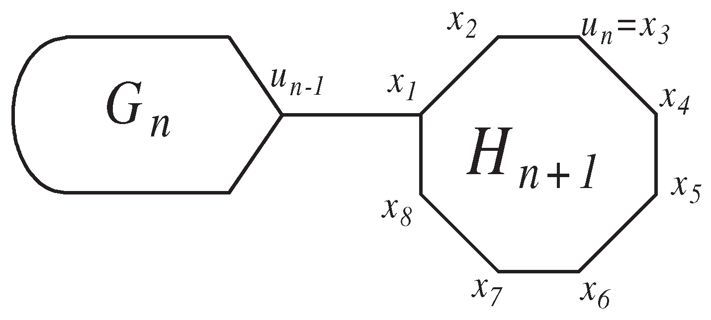
In this paper,we mainly talk about the cyclooctatetraene chain $G_n$ with n octagons, which are constructed by the following way.

Firstly, $G_1$ is an octagon and $G_2$ is the Figure 1 graph with 2 octagons.

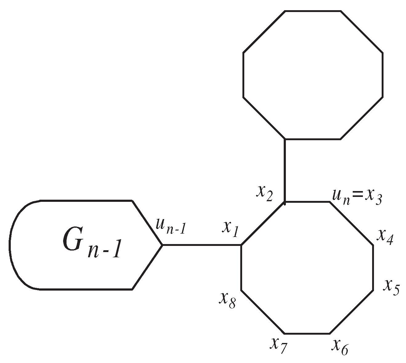
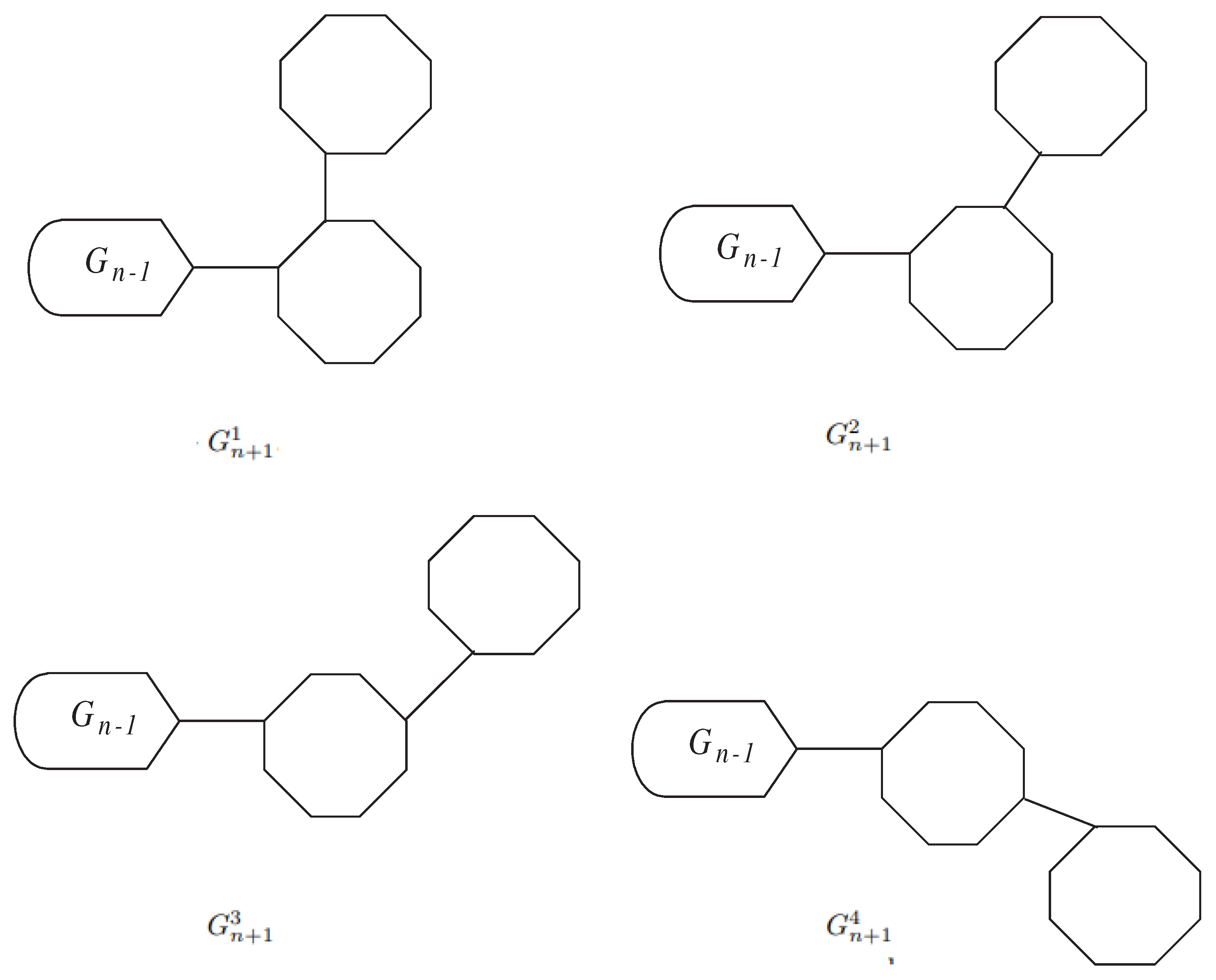
Secondly, The random cyclooctatetraene chain $G_{n+1}$ with n octagons is constructed by attaching a new terminal octagon $H_{n+1}$ to $G_n$. We demonstrate this process by Figure 2. As demonstrated in Figure 3, we can attach the terminal hexagon $H_{n+1}$ to $G_n$ in four ways and denote the resulted figures by $G_{n+1}^1$, $G_{n+1}^2$, $G_{n+1}^3$, $G_{n+1}^4$ respectively.

At each step, a random selection is made from one of the following possible constructions:

We consider four random variables $Z_n^1,Z_n^2,Z_n^3,Z_n^4$ as our choice. If our choice is $G_{n+1}^i$, we let $Z_n^i=1$, otherwise $Z_n^i=0$, $i=1,2,3,4$, we can easily obtain that and $Z_n^1+Z_n^2+Z_n^3+Z_n^4=1$.

By the above processes, we obtain a random polyphenylene chain $G_n(p_1,p_2,p_3,p_4)$. We always abbreviate $G_n(p_1,p_2,p_3,p_4)$ to $G_n$.

Noting that $G_n$ is a random graph, $Gut\left(G_n\right)$, $S\left(G_n\right)$, $K{f}^{*}\left(G_n\right)$ and $K{f}^{+}\left(G_n\right)$ are all random variables in probability. In the view of probability, one problem appears naturally. When n is big enough, whether the distribution of $Gut\left(G_n\right)$, $S\left(G_n\right)$, $K{f}^{*}\left(G_n\right)$ and $K{f}^{+}\left(G_n\right)$ will look like a distribution in probability or not.

In this paper, we make the following hypothesis.

Hypothesis 1.1. Our choice of attaching the new terminal hexagon $H_{n+1}$ to $G_n$, $n=2,3,...$ are random and independently. In more accurate words, the series of random variables ${Z_n^1,Z_n^2,Z_n^3,Z_n^4}_{n=2}^{\infty }$ are independently and have the same law (9). For some $i\in 1,2,3$, we have $0<p_i<1$. Under Hypothesis 1.1, we give analytical expressions for the variances of $Gut\left(G_n\right)$, $S\left(G_n\right)$, $K{f}^{*}\left(G_n\right)$ and $K{f}^{+}\left(G_n\right)$

For a random cyclooctatetraene chain $G_n$, the Gutman index and Schultz index are random variables. In this section, we will consider the variances of $Gut\left(G_n\right)$ and $S\left(G_n\right)$. In fact, $G_{n+1}$ is $G_n$ linked to a new terminal octagon $H_{n+1}$ by an edge, where $H_{n+1}$ is spanned by vertices $x_1$, $x_2$, $x_3$, $x_4$, $x_5$, $x_6$, $x_7$, $x_8$, and the new edge is $u_n{x}_1$; see Figure 1. On the hand, for all $v\in V_{G_n}$, one has On the other hand,

In [40] Theorem 1, the author proves that

Now we introduce the first main result in this section.

Proof. Let then, by [40] (5.1), we obtain

Recalling that $Z_n^1$,$Z_n^2$,$Z_n^3$,$Z_n^4$are random variables in Section 1 which indicate our choice in the construction of $G_{n+1}$ from $G_n$. We have the following four equalities.

Equality 1.

If $Z_n^1=0$, the above equality is obvious. So we only need to consider the case $Z_n^1=1$, which implies $G_n⟶G_{n+1}^1$. In this case, $u_n$ (of $G_n$) coincides with the vertex labelled $x_2$ or $x_8$ (of $H_n$), see Figure 4. In this situation, $A_n$ becomes in the above, we have used (10)-(12). Thus, we conclude the desired equality.

Equality 2.

As that in the proof of Equality 1, we only consider the case $Z_n^2=1$, that is $G_n⟶G_{n+1}^2$. The proof is similar and we omit the details.

Equality 3. we only consider the case $Z_n^3=1$, that is $G_n⟶G_{n+1}^3$. The proof is the same as Equality 1 and we omit the details.

Equality 4. we only consider the case $Z_n^4=1$, that is $G_n⟶G_{n+1}^4$. The proof is also similar and we omit the details.

Noting that $Z_n^1+Z_n^2+Z_n^3+Z_n^4=1$, by the above discussions, it holds that where for each n,

$U_n=648Z_n^1+972Z_n^2+1296Z_n^3+1620Z_n^4,V_n=90Z_n^1+414Z_n^2+738Z_n^3+1062Z_n^4$. Therefore, by (15) we obtain

By direct calculation, one sees that$Var\left(U_j\right)={\sigma }^2$, $Var\left(V_j\right)={\tilde{\sigma }}^2$, $Cov(U_j,V_j)=r$, where for any two random variablesX, Y, $Cov(X,Y):=E\left(XY\right)-E\left(X\right)E\left(Y\right)$. By the properties of variance and interchanging the order of sums, it follows that

With the help of a computer, the above equality implies the desired result $Var\left(Gut\left(G_n\right)\right)$.

Now, we discuss the variance of the Schultz index of a random cyclooctatetraene chain.

In [40] Theorem 2.3, we have Then we state our results.

Proof. by [40] (5.2), we obtain where

With similar discussion, we have the following four equalities.

Equality 1.

If $Z_n^1=0$, the above equality is obvious. So we only need to consider the case $Z_n^1=1$, which implies $G_n⟶G_{n+1}^1$. In this case, $u_n$ (of $G_n$) coincides with the vertex labelled $x_2$ or $x_8$ (of $H_n$),see Figure 4. In this situation, $B_n$ becomes in the above, we have used (10)-(12). Thus, we conclude the desired equality.

Equality 2.As that in the proof of Equality 1, we only consider the case $Z_n^2=1$, that is $G_n⟶G_{n+1}^2$. The proof is similar and we omit the details.

Equality 3. we only consider the case $Z_n^3=1$, that is $G_n⟶G_{n+1}^3$. The proof is the same as Equality 1 and we omit the details.

Equality 4. we only consider the case $Z_n^4=1$, that is $G_n⟶G_{n+1}^4$. The proof is also similar and we omit the details.

Noting that $Z_n^1+Z_n^2+Z_n^3+Z_n^4=1$,by the above discussions, it holds that where for each n,

$U_n=576Z_n^1+864Z_n^2+1152Z_n^3+1440Z_n^4,V_n=40Z_n^1+328Z_n^2+616Z_n^3+904Z_n^4$. Therefore, by (15)

If we replace $Gut\left(G_n\right)$ by $S\left(G_n\right)$ in the proof of Theorem 1, the rest proof of this theorem is the same as that in the proof of Theorem 1 and we omit the details.

In this section, we talk about the variances for $K{f}^{*}\left(G_n\right)$ and $K{f}^{+}\left(G_n\right)$. For a random cyclooctatetraene chain $G_n$, the multiplicative degree-Kirchhoff index $K{f}^{*}\left(G_n\right)$ and the additive degree-Kirchhoff index $K{f}^{+}\left(G_n\right)$ are random variables.

Recall that $G_{n+1}$ is obtained by attaching $G_n$ a new terminal octagon $H_{n+1}$ by an edge, where $H_{n+1}$ is spanned by vertices $x_1$, $x_2$, $x_3$, $x_4$, $x_5$, $x_6$, $x_7$, $x_8$, and the new edge is $u_n{x}_1$; see Figure 1. On the hand, for all $v\in V_{G_n}$, one has

On the other hand,

In [40] Theorem 3, we have

Now we introduce the first main result in this section.

Proof. by [40] (5.3), we see where

Recalling that $Z_n^1,Z_n^2,Z_n^3,Z_n^4$ are random variables in Section 1 which indicate our choice in the construction of $G_{n+1}$ from $G_n$. We have the following four equalities.

Equality 1.

If $Z_n^1=0$, the above equality is obvious. So we only need to consider the case $Z_n^1=1$, which implies $G_n⟶G_{n+1}^1$. In this case, $u_n$ (of $G_n$) coincides with the vertex labelled $x_2$ or $x_8$ (of $H_n$), see Figure 4. In this situation, $C_n$ becomes in the above, we have used (17)-(19). Thus, we conclude the desired equality.