VaR Estimation Using Extreme Value Mixture Models for Cryptocurrencies

Cryptocurrencies have obtained a crucial position in the international financial landscape. The cryptocurrency market has been perceived as a highly volatile market since the inception of Bitcoin. This study investigates the relevant performance of extreme value models (EVM) in estimating the Value-at-Risk (VaR) of Bitcoin and Ethereum returns. The extreme value mixture models, GPD-Normal-GPD (GNG) and GPD-KDE-GPD models are fitted to the returns of Bitcoin and Ethereum and the Kupiec likelihood backtesting procedure is performed on the VaR estimates to assess the fits. Both models’ results showed that the fits were a much more decent representation of the observed data when compared to the Normal distribution. The backtesting results showed that the GPD-KDE-GPD model’s fit was superior to that of the GPD-Normal-GPD for both sets of returns at all VaR risk levels except at the 99% level. The results of this study may assist with understanding the dynamics and risks associated with cryptocurrencies and can serve as a beneficial tool for decision-making and risk management to investors, traders, financial institutions and many other participants in the cryptocurrency ecosystem.

Keywords:

Bitcoin

;

cryptocurreny

;

extreme value models (EVM)

;

GPD-Normal-GPD (GNG)

;

generalised Pareto distribution (GPD)

;

Kernel density estimator (KDE)

;

Normal distribution

;

Value-at-Risk (VaR)

Subject:

Business, Economics and Management - Econometrics and Statistics

1. Introduction

The cryptocurrency market is a developing high volatile market since the introduction of it’s most prominent constituent, Bitcoin, in 2008 by Satoshi Nakamoto. Thereafter, the cryptocurrency market has gained much interest from the media, policymakers, investors, government institutions, academicians, regulators and the general public. The second largest cryptocurrency is Ethereum, which was first incepted in 2015 and now has a substantial market share.

Due to the absence of a central bank issuing cryptocurrencies, they have no exposure to the common stock markets and thus typical factors like inflation and interest rates have no affect on the cryptocurrency market. However, cryptocurrency prices are influenced by multiple other factors which include economic and political events, the creation of new currencies, government regulations, speculation, hacking, news, and mutual influence [18]. Consequently, the cryptocurrency market is considered more volatile and riskier than traditional fiat currency markets and also exhibit heavier tail behaviour.

The extreme changes observed in cyrptocurrency returns breach the assumptions of normality which has created a great demand to appropriately model the behaviour of these returns as it plays a crucial role in risk management and prediction of market losses [12].

It was first considered by [14] to apply the extreme value theory (EVT) to provide a simple way to assess the characteristics of the distribution tails of asset returns. However, limited studies, to date, has utilised extreme value theory for cryptocurrencies to examine the tail behaviour and the extremities related to it’s returns.

[17] used an extreme value approach to analyse Bitcoin returns and found that Bitcoin is, in fact, more volatile and riskier than traditional currencies. The study was then furthered to analyse five more cryptocurrencies using the extreme value method. They were able to show that all the cryptocurrencies investigated were also more volatile and riskier, however, Bitcoin was the least risky when compared to the others.

[12] employed the extreme value theory to assess the tail behaviour of the five largest cryptocurrencies’ returns. The analysis was performed by fitting a Generalised Pareto distribution (GPD) to the marginal distribution of the all five cryptocurrency returns. They then estimated the measures of Value-at-Risk (VaR) and Expected Shortfall (ES) as extreme quantiles of the GPD. It was concluded that Bitcoin cash is the riskiest and Bitcoin and Litecoin were the least risky cryptocurrencies.

[7] employed the GPD model to examine the estimation of VaR and ES and compared the riskiness of Bitcoin (BTC/USD) to the South African rand (ZAR/USD). The Bitcoin returns exhibited heavy-tail behaviour in both gains and losses indicating that the GPD is a great model offering an apt fit for the tails’ distribution. The study concluded that the Bitcoin gave higher returns but is also much riskier than the South African rand.

[13] modelled the daily Bitcoin returns using the GPD. Their findings show that EVT was able to capture the extreme returns and uncertainty of Bitcoin and adequately explain the tails’ behaviour in the cryptocurrency market.

The aim of this paper is to estimate VaR values of Bitcoin and Ethereum using extreme value mixture models. A GPD model is fitted to the values of the returns that exceed certain thresholds. Thus, two extreme value mixture models are fitted to both the cryptocurrencies’ returns. GPD-normal-GPD (GNG) model and GPD-KDE-GPD are fitted to both cryptocurrnecy returns.

The VaR estimates are backtested using the Kupiec likelihood ration test to assess the model adequacy of both these fits to the returns. This study can help investors, traders and various other stakeholders in the cryptocurrency ecosystem understand the extremities and risks associated with these cryptocurrencies.

2. Materials and Methods

Extreme value theory is a statistical field of study that focuses on the behaviour of the extremes of a process/processes [9]. This theory is used to derive models that captures the stochastic behaviour of these extreme events in the tails of probability distributions.

2.1. Extreme value mixture models

Extreme value mixture models can be described by two parts. The first part being a bulk model, which is generally a parametric or non-parametric model, that fits the non-external data that are below a given threshold and the second part being the tail model, which describes the data above that threshold. The tail model is usually an easily adaptable model.

2.1.1. Generalised Pareto Distribution (GPD)

A highly suggested threshold excess model is the generalised Pareto distribution (GPD). For a sequence of independent and identically distributed observations,

X_{1}, \dots, X_{n}

,10] described that under given mild conditions, the excess

X - u

over an appropriate u can be estimated by the generalized Pareto distribution, denoted

G (x | u, σ_{u}, ξ)

is given by,

G (x | u, σ_{u}, ξ) = \{\begin{matrix} 1 - {[1 + ξ (\frac{x - u}{σ_{u}})]}_{+}^{- \frac{1}{ξ}} & ξ \neq 0, \\ 1 - exp {[- (\frac{x - u}{σ_{u}})]}_{+} & ξ = 0 \end{matrix}

(1)

where

x > u

σ_{u} > 0

and

[1 + ξ (\frac{x - u}{σ_{u}})] > 0

2.1.2. Threshold Choice

The selection of an appropriate threshold is of critical importance as it segments the extreme and non-extreme values. This process is still a topic of ongoing research, however, [9] noted that the threshold choice procedure always causes a trade-off between the bias and variance. In extreme value modelling methods, a fixed threshold approach is utilised where the threshold is selected and fixed prior to fitting the model. Diagnostic plots are generally used to choose the threshold. These plots include the mean residual life plot, parameter stability plot and numerous general model fit diagnostics plots.

2.1.3. GPD-Normal-GPD (GNG)

A two-tail mixture model was proposed by [19] which makes use of the normal distribution to describe the bulk model and the GPD model is fitted to each tail, separately.

Bulk model based tail fraction method

The GNG distribution is given by,

$F (x | Θ) = \{\begin{cases} ϕ_{u_{l}} [1 - G (- x | - u_{l}, σ_{u_{l}}, ξ_{l})] x < u_{l}, \\ H (x | μ, β) u_{l} \leq x \leq u_{r}, \\ (1 - ϕ_{u_{r}}) + ϕ_{u_{r}} G (x | u_{r}, σ_{u_{r}}, ξ_{r}) x > u_{r} \end{cases}$

(2)

where, $Θ = (u, β, u_{l}, σ_{u_{l}}, ξ_{l}, u_{r}, σ_{u_{r}}, ξ_{r})$ is the parameter vector, $ϕ_{u_{l}} = H (u_{l} | μ, β)$ and $ϕ_{u_{r}} = 1 - H (u_{r} | μ, β)$ and $H (. | μ, β)$ is the normal distribution with mean $μ$ and standard deviation $β$ . The lower and upper tail functions of the GPD are $G (. | - u_{l}, σ_{u_{l}}, ξ_{l})$ and $G (. | u_{r}, σ_{u_{r}}, ξ_{r})$ where $ξ, σ$ and u are the shape, scale and threshold parameters, respectively.
Parameterised tail fraction method

It is also possible to define $ϕ_{u_{l}} = P (X < u_{l})$ and $ϕ_{u_{r}} = P (X > u_{r})$ , and thus the associated distribution is as follows,

$F (x | Θ) = \{\begin{cases} ϕ_{u_{l}} [1 - G (- x | - u_{l}, σ_{u_{l}}, ξ_{l})] x < u_{l}, \\ ϕ_{u_{l}} + (1 - ϕ_{u_{l}} - ϕ_{u_{r}}) \frac{H (x | μ, β) - H (u_{l} | μ, β)}{H (u_{r} | μ, β) - H (u_{l} | μ, β)} u_{l} \leq x \leq u_{r}, \\ (1 - ϕ_{u_{r}}) + ϕ_{u_{r}} G (x | u_{r}, σ_{u_{r}}, ξ_{r}) x > u_{r} \end{cases}$

(3)

where, $Θ = (u, β, u_{l}, σ_{u_{l}}, ξ_{l}, u_{r}, σ_{u_{r}}, ξ_{r})$ is the parameter vector.

2.1.4. GPD-KDE-GPD

[16] introduced a standard kernel GPD mixture model where a standard kernel density estimator is used as the bulk model below the threshold with GPD for the tail model and then went on further to propose a two tailed mixture model by combining the standard kernel density estimator with two extreme value tail models.

Bulk model based tail fraction method

The GPD-KDE-GDP is defined as follows,

$F (x | Θ) = \{\begin{cases} ϕ_{u_{l}} [1 - G (- x | - u_{l}, σ_{u_{l}}, ξ_{l})] & x < u_{l}, \\ H (x | X, λ) & u_{l} \leq x \leq u_{r}, \\ (1 - ϕ_{u_{r}}) + ϕ_{u_{r}} G (x | u_{r}, σ_{u_{r}}, ξ_{r}) & x > u_{r} \end{cases}$

(4)

where, $Θ = (X, λ, u_{l}, σ_{u_{l}}, ξ_{l}, u_{r}, σ_{u_{r}}, ξ_{r})$ is the parameter vector. $ϕ_{u_{l}} = H (u_{l}, X, λ)$ and is approximated as the sample proportions less than the threshold $u_{l}$ and similarly $ϕ_{u_{r}} = 1 - H (u_{r}, X, λ)$ is estimated as the sample proportions greater than the threshold $u_{l}$ . The lower and upper tail unconditional GPD functions are $G (. | - u_{l}, σ_{u_{l}}, ξ_{l})$ and $G (. | u_{r}, σ_{u_{r}}, ξ_{r})$ where $ξ, σ$ and u are the shape, scale and threshold parameters, respectively.
Parameterised tail fraction method

The parameterised distribution function is given by,

$F (x | Θ) = \{\begin{cases} ϕ_{u_{l}} [1 - G (- x | - u_{l}, σ_{u_{l}}, ξ_{l})] & x < u_{l}, \\ ϕ_{u_{l}} + (1 - ϕ_{u_{l}} - ϕ_{u_{r}}) \frac{H (x | X, λ) - H (u_{l} | X, λ)}{H (u_{r} | X, λ) - H (u_{l} | X, λ)} & u_{l} \leq x \leq u_{r}, \\ (1 - ϕ_{u_{r}}) + ϕ_{u_{r}} G (x | u_{r}, σ_{u_{r}}, ξ_{r}) & x > u_{r} \end{cases}$

(5)

where, $Θ = (u, β, u_{l}, σ_{u_{l}}, ξ_{l}, u_{r}, σ_{u_{r}}, ξ_{r})$ is the parameter vector.

A parameterised tail fraction approach is performed in this study to estimate the parameters of the GNG and GPD-KDE-GPD models fitted to both Bitcoin and Ethereum returns data. The evmix package in the statistical software platform R is used to apply the methods required to achieve the results in the following sections.

2.2. Value-at-Risk and Backtesting

In market risk management, Value-at-risk (VaR), is one of the most frequently used risk metric. VaR summarises the statistical measures of potential losses and is often indicated as a confidence interval in the units of a specified currency over a certain time period [16]. VaR can be defined as follows,

VaR (p) = {\hat{O}}^{- 1} (p)

(6)

where cumulative distribution function (CDF) of the best fitting distribution is given by

\hat{O} (.)

for

0 < p < 1

VaR backtesting methods assess the coverage of the unconditional and conditional left-tail of a log returns distribution [1] and thus provides a more formal approach to evaluate model adequacy and robustness. The Kupiec likelihood ratio test was first considered by [15] and the conditional coverage test was first considered by [8]. In this paper, we make use of the Kupiec likelihood ratio test for backtesting.

3. Results

3.1. Data source and description

Daily Bitcoin and Ethereum closing prices in United States dollars (USD) are used in this study. The periods used for each cryptocurrency differs due to data limitations. For the Bitcoin closing prices, 2558 observations were used which was recorded over the 7 year period of 28/07/2015-28/07/2022 whereas 1723 observations of the Ethereum closing prices were used for the period 09/11/2017-28/07/2022. The datasets were obtained from: https://www.cryptodatadownload.com/data/northamerican/.

Figure 1 presents the time series plots of the daily Bitcoin prices (USD) and the daily Ethereum prices (USD). The plots show rather volatile trends over the periods analysed for both cryptocurrency prices which implies non-constant means and high variability. This indicates non-stationarity of the cryptocurrency prices. Since returns on investment are the interest of most investors, the closing prices of the cryptocurrencies’ were transformed to log returns,

r_{t}

, as follows,

r_{t} = ln \frac{p_{t}}{p_{t - 1}}

(7)

where

p_{t}

is the closing price of the cryptocurrency at time t, and

p_{t - 1}

is the closing price of the cryptocurrency at time

t - 1

Figure 2 shows the time series plots of the transformed log returns. Both returns’ trends appear to be fluctuating around zero implying that the data is now stationary in mean. Trends of high and low periods are still observed to be prominent indicating the presence of time-varying variances. Such behaviour is consistent with that of volatility clustering and leverage effects.

The descriptive statistics of the Bitcoin and Ethereum returns are recorded in Table 1. The mean of the Bitcoin returns is insignificantly greater than zero but this implies that the returns are slightly increasing. The Ethereum returns’ mean, however, is slightly less than zero indicating that over the period studied, the returns may be decreasing. Bitcoin appears to be negatively skewed whereas Ethereum is positively skewed. Thus the Bitcoin returns have a larger left tail implying that the returns’ losses are greater than the profits and since Ethereum returns have a larger right tail, the converse applies. Positive excess kurtosis are observed for both cryptocurrencies’ returns which is consistent with characteristics of financial data.

Table 2 records the formal tests applied to the Bitcoin and Ethereum returns. In order to evaluate the stationarity of the daily returns of Bitcoin and Ethereum, three cases of the ADF test, the PP test and the KPSS test were utilised. The p-values of all three cases of the ADF and PP tests both cryptocurrencies’ returns are less than 0.05, thus the null hypothesis of non-stationarity can be rejected at a 5% level of significance. The KPSS test which has a null hypothesis of stationarity, produce p-values greater than 0.05 for both sets of returns. This supports the results of the ADF and PP tests suggesting stationarity in the returns as we fail to reject the null hypothesis.

Two tests of normality were performed on the returns- the Jarque-Bera and Shapiro Wilk tests. The resultant p-values for both sets of returns were less than 0.05, thus rejecting the null hypothesis of normality at a 5% level of significance.

The Cox-Stuart test was used to explore the time variation in the Bitcoin and Ethereum returns. The p-values of the test were greater than 0.05 for both sets of returns and thus the null hypothesis of a non-monotonic trend fails to be rejected at a 5% level of significance.

The Ljung-Box test performed on the Bitcoin and Ethereum returns produces p-values greater than 0.05 implying that the null hypothesis of no serial correlation fails to be rejected at a 5% level of significance. However, the ARCH-LM test shows that there is a presence of strong ARCH effects in both the Bitcoin and Ethereum returns.

The results of the exploratory data analysis concludes that the daily Bitcoin and Ethereum returns exhibit empirical traits such as heavy-tails, volatility clustering and non-linear dependence, significant serial correlations in the absolute and squared returns, time variation, leverage effects and ARCH effects.

3.2. Fitting the extreme value mixture models

Two extreme value mixture models were fitted to the daily returns of Bitcoin and Ethereum. The parameter estimates of the GPD-Normal-GPD and GPD-KDE-GPD are reported in Table 3.

Figure 3 and Figure 4 show the density histograms of the Bitcoin (a) and Ethereum (b) returns overlaid with the fitted extreme value mixture models. As observed in Figure 3, the GPD-Normal-GPD is a good fit to both sets of the cryptocurrency returns and a much better fit when compared to the Normal distribution. In Figure 4, it is apparent that the GPD-KDE-GPD model is the best fit to the data when compared to the Normal distribution as well as the KDE model without the GPD tails. Deducing that these models are a good fit from just examining the fitted plots is not substantial enough to conclude that these models are in fact adequate fits. Thus, a formal approach applying VaR estimation and the Kupiec likelihood ratio test was used to verify that these extreme value mixture models are appropriate fits.

3.3. VaR estimation

A common risk measure that is of interest to traders are the Value-at-Risk (VaR) estimates as it enables them to evaluate the risks that are linked with their portfolios’ future values and thus allowing them to take into consideration any potential losses. It is estimated at long positions of 1%, 2.5% and 5% as well as short positions of 95%, 97.5% and 99%. Table 4 shows the VaR estimates for the long and short positions. For the Bitcoin returns, the GPD-Normal-GPD produced the lowest VaR estimates at all 3 long positions and the 95% short position. The GPD-KDE-GPD produced the lowest VaR estimates at the other two short positions.

3.4. Backtesting

Backtesting was performed using the Kupiec likelihood ratio test (1995) to assess the model adequacy in VaR estimation. Table 5 shows the resultant p-values of the Kupiec likelihood ratio test at the long and short positions. For both sets of returns, the GPD-KDE-GPD model produced a p-value greater than 0.05 at all levels of risk. This indicates that we fail to reject the null hypothesis of model adequacy and confirm that this mixture model is an appropriate fit for both the Bitcoin and Ethereum returns. The p-values of the GPD-Normal-GPD for the 1% long position for Bitcoin and for the 2.5% long position for Ethereum are less than 0.05. Thus we reject the null hypothesis at a 5% level of significance and can conclude that the model may be a misfit for the returns at these risk levels. However, at all other levels of the long and short positions, it appears that model is an adequate fit.

4. Conclusions

Financial decisions are strongly influenced by understanding the risks that are associated with returns. There has been numerous methods proposed but are only applicable if the normality assumptions are valid. Research and studies have shown that EVT is a better approach to grasp the nature of tail returns. EVT can be used to explain erratic behaviour of returns that may be exhibited due to extreme events, like the recent COVID-19 pandemic, when compared to other approaches. The studies of cryptocurrencies’ extreme returns/tails distributions are rather limited as most research’s focus is the entire distribution. The empirical analysis carried out in this paper utilises extreme value mixture models fitted to two of the largest cryptocurrencies’ returns, Bitcoin and Ethereum.

A GNG model and GPD-KDE-GPD model were applied to both sets of returns. The results of the two extreme value mixture models depicted satisfactory representations of the observed data. Backtesting was performed on the VaR estimates using the Kupiec likelihood ratio test to assess the model adequacy of the fitted distributions. Excellent results were found for the GPD-KDE-GPD models fitted to both sets of returns as the model was adequate at all risk levels investigated in this paper. The GNG model, however, showed mixed results but proved to be appropriate fits at majority of the risk levels for both cryptocurrencies’ returns.

The findings in this paper may have crucial implications to investors, traders regulators and policy-makers, financial institutions and various other stakeholders in the cryptocurrency markets as it can assist them with a greater understanding of their investments, especially when these investments are exposed to extreme events.

Further research can comprise of the exploration of different bulk models fitted to these two cryptocurrencies’ to make comparisons on the models investigated in this study. Also, the extreme value mixture models used here can be applied to numerous other cryptocurrencies to evaluate the risks that are associated with each of them.

References

Ardia, D.; Boudt, K.; Catania, L. Generalized Autoregressive Score Models in R: The GAS Package. Papers, arXiv.org. 2016. [Google Scholar]
Bhosale, J. & Mavale, S. Volatility of select Crypto-currencies: A comparison of Bitcoin, Ethereum and Litecoin. Annual Research Journal of SCMS 2018, 6, 132–141.
Bouoiyour, J. , Selmi, R., Tiwari, A., & Olayeni, O. What drives Bitcoin price? Economics Bulletin 2016, 36, 843–850.
Catania, L. & Grassi, S. Modelling Cryptocurrencies Financial Time Series SSRN Electronic Journal. 2017. [Google Scholar]
Chan, S. , Chu, J., Zhang, Y., & Nadarajah, S. An extreme value analysis of the tail relationships between returns and volumes for high frequency cryptocurrencies. Research in International Business and Finance. 2022; 59.
Chan, S. , Chu, J. , Nadarajah, S., & Osterrieder, J. A Statistical Analysis of Cryptocurrencies. In Journal of Risk and Financial Management 2017, 10(2), 12. [Google Scholar]
Chikobvu, D.; Ndlovu, T. The Generalised Extreme Value Distribution Approach to Comparing the Riskiness of BitCoin/US Dollar and South African Rand/US Dollar Returns. Risk Financial Manag. 2023, 16, 253. [Google Scholar] [CrossRef]
Christoffersen, P. Evaluating Interval Forecasts. International Economic Review 1998, 39, 841–862. [Google Scholar] [CrossRef]
Coles, S. , 2001 An introduction to statistical modeling of extreme values. In Springer Series in Statistics.
Davison, A. C. , & R. L. Smith., Models for Exceedances over High Thresholds. Journal of the Royal Statistical Society. Series B (Methodological). 1990, pp. 393–442, JSTOR. Available online: http://www.jstor.org/stable/2345667.
Duffie, D. , & Pan, J. , An overview of value at risk. Journal of derivatives 1997, 4(3), 7–49. [Google Scholar]
Gkillas, K. & Katsiampa, P. An application of extreme value theory to cryptocurrencies. Economics Letters, 2018; 164.
Hussain, S.I.; Masseran, N.; Ruza,, N.; Safari, M.A.M. Predicting Extreme Returns of Bitcoin: Extreme Value Theory Approach . Journal of Physics: Conference Series 2021, 1988, 012091. [Google Scholar]
Longin, F. The choice of the distribution of asset returns: How extreme value theory can help? Journal of Banking & Finance, 2005; 29, 4. [Google Scholar] [CrossRef]
Kupiec, P. Techniques for Verifying the Accuracy of Risk Measurement Models Journal of Derivatives 1995, 3, 73-84. [CrossRef]
MacDonald, A.; Scarrott C.J.; Lee D.; Darlow B.; Reale M.; Russel G. A flexible extreme value mixture model. Computational Statistics & Data Analysis, 2011; 2137–2157. [CrossRef]
Osterrieder, J.; Lorenz, J. A statistical risk assessment of Bitcoin and its extreme tail behavior. Annals of Financial Economics 12(01), 2017 p.1750003.
Vaz de Melo Mendes, B.; Fluminense Carneiro, A. A Comprehensive Statistical Analysis of the Six Major Crypto-Currencies from August 2015 through June 2020. Risk Financial Manag. 2020, 13, 192. [Google Scholar] [CrossRef]
Zhao, X., Scarrott, C., Oxley, L. & Reale, M. Extreme value modelling for forecasting market crisis impacts. Applied Financial Economics. 2010, 20, 63–72.

Figure 1. Time series plots of (a) daily Bitcoin prices (USD) for the period 28/07/2015-28/07/2022, (b) daily Ethereum prices (USD) for the period 09/11/2017-28/07/2022.

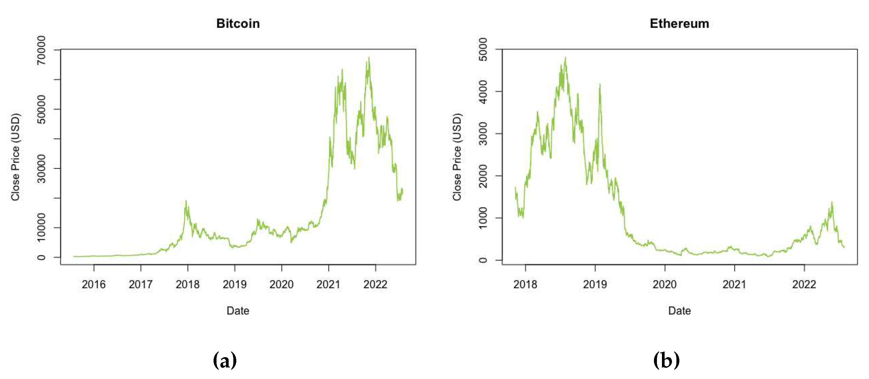
Figure 2. Time series plots of (a) daily Bitcoin log returns for the period 28/07/2015-28/07/2022, (b) daily Ethereum log returns for the period 09/11/2017-28/07/2022.

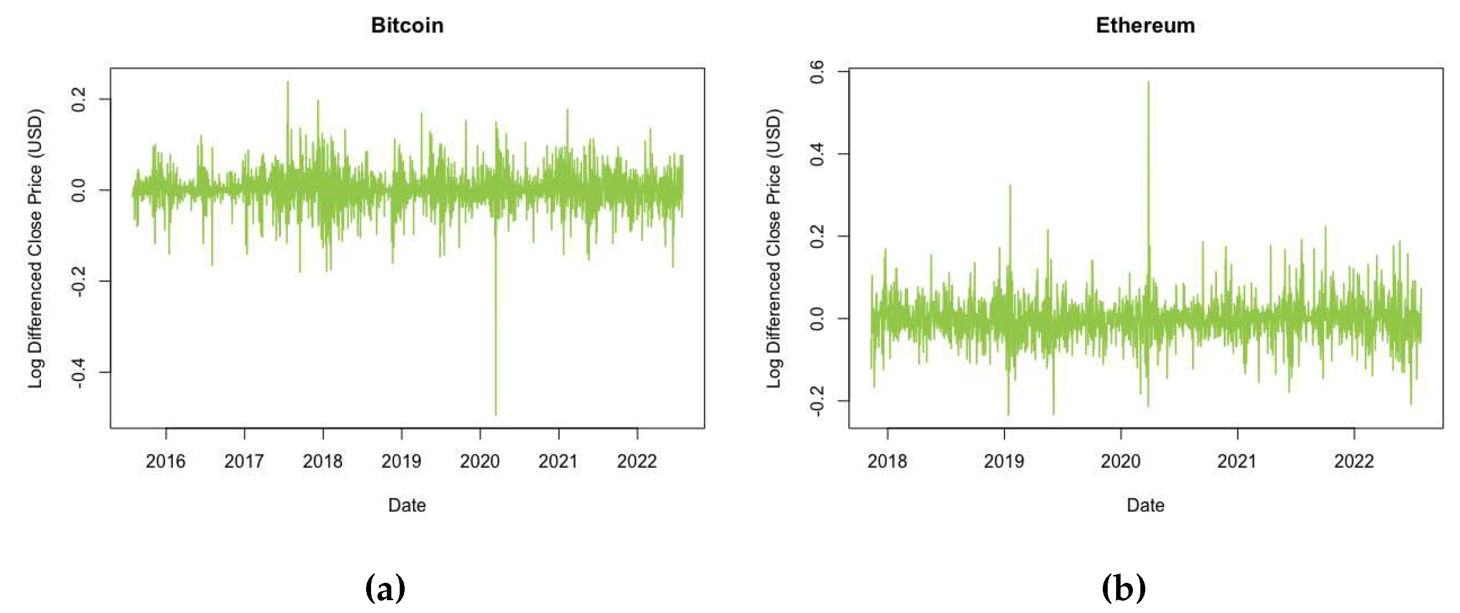
Figure 3. Histogram of (a) Bitcoin and (b) Ethereum daily returns data overlaid with a fitted two tailed Normal GPD model for bulk.

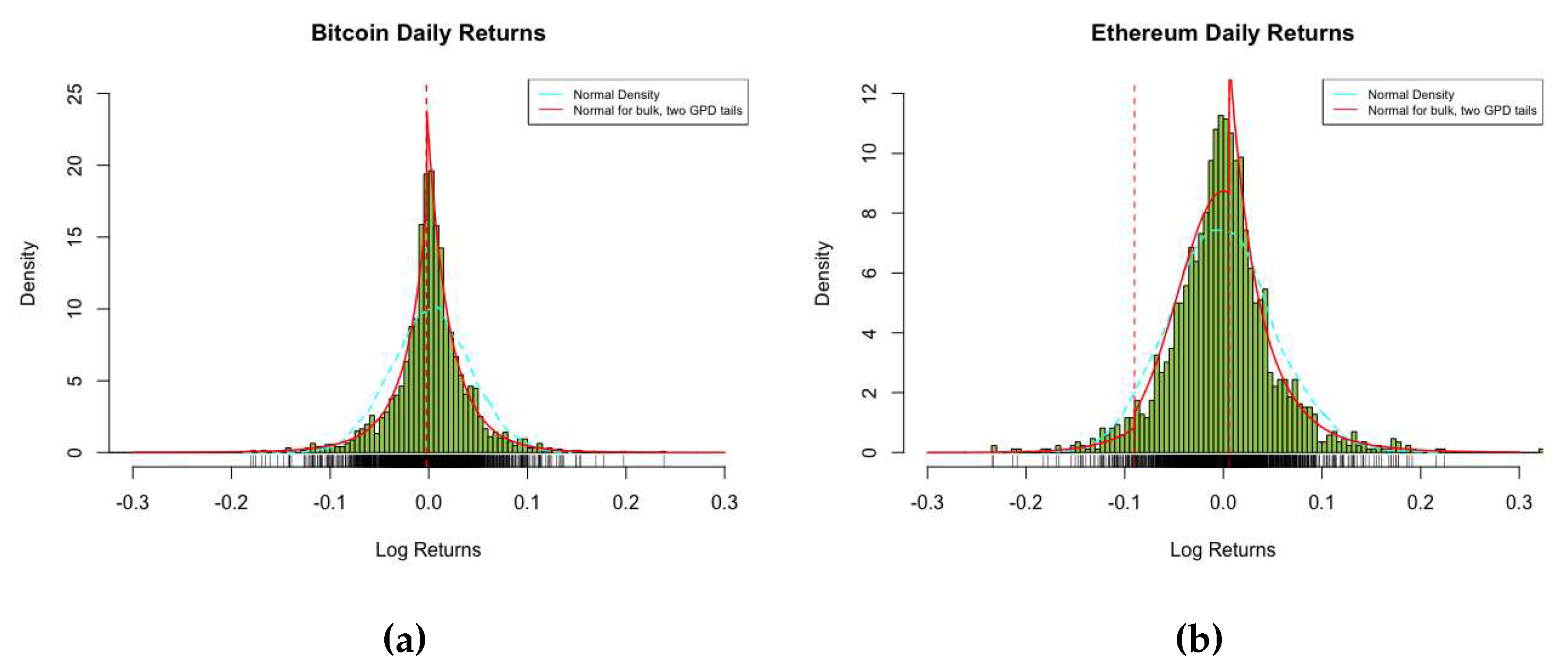
Figure 4. Histogram of (a) Bitcoin and (b) Ethereum daily returns data overlaid with a fitted two tailed kernel GPD model and a Gaussian KDE model for bulk.

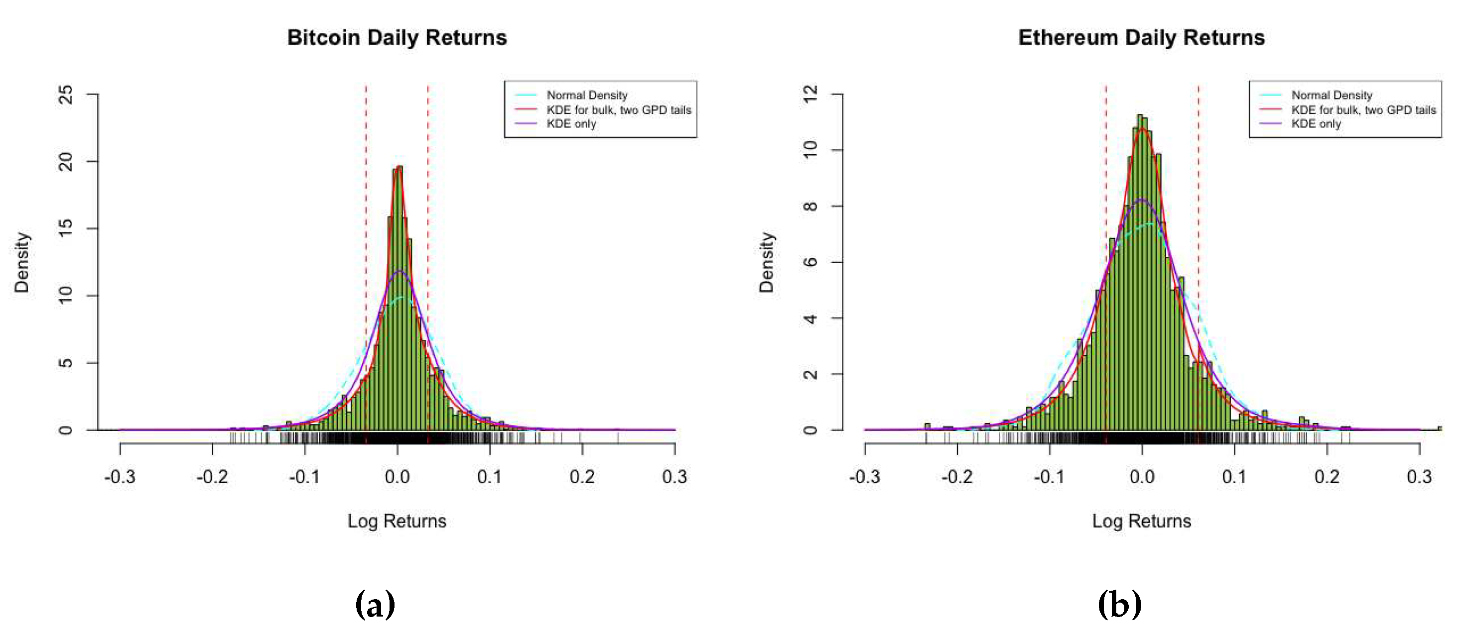
Table 1. Descriptive statistics of the log returns of the daily Bitcoin and Ethereum prices.

Statistics	Bitcoin	Ethereum
Minimum	-0.4940	-0.2341
Maximum	0.2384	0.5756
Mean	0.0017	-0.0010
STDEV	0.0400	0.0535
Skewness	-0.8019	0.9219
Kurtosis	11.9492	9.9282

Table 2. Formal tests of the log returns of daily Bitcoin prices (BTC/USD) and Ethereum prices (ETH/USD)

		Bitcoin		Ethereum
Test		Test Statistic	p-value	Test Statistic	p-value
Stationarity	ADF test
	Case 1: No drift, no trend	-14.2000	0.0100	-11.8000	0.0100
	Case 2: Drift, no trend	-14.3000	0.0100	-11.8000	0.0100
	Case 3: Drift and trend	-14.4000	0.0100	-11.8000	0.0100
	PP test
	Case 1: No drift, no trend	-2845.0000	0.0100	-2023.0000	0.0100
	Case 2: Drift, no trend	-2834.0000	0.0100	-2022.0000	0.0100
	Case 3: Drift and trend	-2830.0000	0.0100	-2022.0000	0.0100
	KPSS test
	Case 1: No drift, no trend	2.6000	0.0137	0.4760	0.1000
	Case 2: Drift, no trend	0.2300	0.1000	0.1770	0.1000
	Case 3: Drift and trend	0.0777	0.1000	0.1420	0.0571
Normality	Jarque-Bera test	15516.0000	$< 0.0001$	7338.2000	$< 0.0001$
Normality	Shapiro-Wilk	0.9127	$< 0.0001$	0.9344	$< 0.0001$
Time variation	Cox-Stuart test	605.0000	0.0609	452.0000	0.1523
Autocorrelation	Ljung-Box test	15.4790	0.0303	63.1450	0.1003
ARCH effects	Box-Ljung test	15.4790	0.0303	63.1450	0.1003
ARCH effects	ARCH-LM test	25.4960	$< 0.0001$	21.2320	$< 0.0001$

Table 3. Estimation of results of the GPD-Normal-GPD and GPD-KDE-GPD models for the Bitcoin and Ethereum daily returns.

Distribution	Parameter estimates	Bitcoin	Ethereum
GPD-Normal-GPD
	$\hat{μ}$	0.0019	-0.0012
	$\hat{β}$	0.0212	0.0464
	$\hat{μ_{l}}$	-0.0026	-0.0901
	$\hat{σ_{μ_{l}}}$	0.0247	0.0335
	$\hat{ξ_{l}}$	0.1587	-0.0407
	$\hat{ϕ_{μ_{l}}}$	0.4153	0.0278
	$\hat{μ_{r}}$	-0.0020	0.0059
	$\hat{σ_{μ_{r}}}$	0.0240	0.0331
	$\hat{ξ_{r}}$	0.0779	0.0983
	$\hat{ϕ_{μ_{r}}}$	0.5734	0.4387
GPD-KDE-GPD
	$\hat{λ}$	0.0032	0.0075
	$\hat{μ_{l}}$	-0.0342	-0.0393
	$\hat{σ_{μ_{l}}}$	0.0304	0.0334
	$\hat{ξ_{l}}$	0.0707	0.0015
	$\hat{ϕ_{μ_{l}}}$	0.1246	0.1913
	$\hat{μ_{r}}$	0.0328	0.0609
	$\hat{σ_{μ_{r}}}$	0.0270	0.0312
	$\hat{ξ_{r}}$	0.0242	0.2091
	$\hat{ϕ_{μ_{r}}}$	0.1541	0.0950

Table 4. VaR estimates for the Bitcoin and Ethereum returns at long and short positions

	Distribution	Long position			Short position
	Distribution	1%	2.5%	5%	95%	97.5%	99%
Bitcoin	GPD-Normal-GPD	-0.1279	-0.0899	-0.0646	0.0625	0.0832	0.1123
Bitcoin	GPD-KDE-GPD	-0.1182	-0.0859	-0.0629	0.0636	0.0830	0.1092
Ethereum	GPD-Normal-GPD	-0.1237	-0.0937	-0.0776	0.0860	0.1154	0.1574
Ethereum	GPD-KDE-GPD	-0.1380	-0.1073	-0.0841	0.0823	0.1090	0.1507

Table 5. VaR backtesting for the Bitcoin and Ethereum returns

	Distribution	Long position			Short position
	Distribution	1%	2.5%	5%	95%	97.5%	99%
Bitcoin	GPD-Normal-GPD	0.0119	0.3717	0.5307	0.7079	0.4484	0.9321
Bitcoin	GPD-KDE-GPD	0.3486	0.8064	0.6424	0.9891	0.4484	0.6343
Ethereum	GPD-Normal-GPD	0.1830	0.0016	0.0549	0.3059	0.5254	0.9574
Ethereum	GPD-KDE-GPD	0.7649	0.8838	0.6685	0.8342	0.5479	0.6715

Disclaimer/Publisher’s Note: The statements, opinions and data contained in all publications are solely those of the individual author(s) and contributor(s) and not of MDPI and/or the editor(s). MDPI and/or the editor(s) disclaim responsibility for any injury to people or property resulting from any ideas, methods, instructions or products referred to in the content.

© 2023 by the authors. Licensee MDPI, Basel, Switzerland. This article is an open access article distributed under the terms and conditions of the Creative Commons Attribution (CC BY) license (http://creativecommons.org/licenses/by/4.0/).

Copyright: This open access article is published under a Creative Commons CC BY 4.0 license, which permit the free download, distribution, and reuse, provided that the author and preprint are cited in any reuse.

Downloads

154

Views

Comments

Subscription

Notify me about updates to this article or when a peer-reviewed version is published.

MDPI Initiatives

Important Links

Choose an area of interest and we will send you notifications of new preprints at your preferred frequency.

Disclaimer