1. Introduction
As an important evaluation method, the comprehensive evaluation model has been widely applied in various fields, such as ecological civilization development level [
1], environmental evaluation [
2], ecosystem stability assessment [
3] and water quality pollution evaluation [
4]. This evaluation model can help researchers to quantify the environment system comprehensively. However, the practical environmental system is complex and its determining factors are often interrelated. Therefore, a single factor evaluation is insufficient to assess the status of practical system. However, most comprehensive evaluation models are usually used to assess single-factor systems, which fail to accurately capture the complexity of practical environmental systems [
5]. Thus, the developing of effective evaluation model for multi-factors system is a crucial challenge.
In order to solve these issues and improve the performance of assessment, various methods have been proposed [
6,
7,
8,
9,
10,
11]. The traditional entropy weight (TEW) method has been proposed to obtain an objective weight based on the uncertainty of information. However, in situations where the differences in entropy are small, this method may yield excessively high weight values [
12]. These results indicated that the TEW method has poor resistance to extreme values (data with a small difference in entropy). To effectively reduce the weight differences and enhance the resistance to extreme data, the improved entropy weight (IEW) method has been proven to optimize the entropy evaluation formula [
13,
14,
15,
16,
17,
18]. However, this method resulted in overcorrection of normal data weight, causing it to deviated from the law of consistency in entropy weight variation. Besides, this method is typically used in conjunction with single-factor evaluation (SFE) method, which is particularly suitable for systems with fewer or independent factors. But, for a complex systems with multiple factors, the SFE method may lack rationality due to the interrelationship between these factors. The fuzzy comprehensive evaluation (FCE) method utilizes the membership degree theory of fuzzy mathematical model to transform qualitative assessments into quantitative ones, can effectively evaluate complex environmental systems that are influenced by multiple predetermined factors [
19,
20,
21,
22,
23,
24,
25]. However, literature [
26,
27] have pointed that the FCE method is greater subjectivity in weight determination, which results in lower accuracy of evaluation results.
In this paper, we establish an optimized improved entropy weight (OIEW) model and integrate it with the FCE method to achieve multi-factors system assessment. To improve the accuracy of weight determination and enhance the anti-interference ability in handling extreme data, we develop an objective function based on the law of consistency in entropy weight variation using the mathematical programming concepts. This single objective model can be effectively solved by the linear programming algorithm, which prevents normal data from being suppressed. Furthermore, our model can effectively realize the comprehensive evaluation of multi-factors system by integrating the FCE method. The theoretical and simulation results demonstrate that our model can enhance the precision of weight determination and evaluation outcomes. Our works provide theoretical guidance for the practical application in the complex system evaluation field.
2. Disadvantages of entropy evaluation method
The traditional entropy evaluation (TEW) method is an objective weighting method that employs the calculation of information entropy value (IEV) to determine the weight of each factor. In the calculation process, the evaluation results follow the law of consistency in entropy weight variation, whereby an increase in IEV corresponds with decrease the weight, and vice versa [
28] (The detail calculation process see Appendix A). However, this method has poor resistance to extreme data and is greatly affected by outliers. To overcome this limitation, several studies [
15,
16,
17,
18] have proposed by incorporating a correction factor to enhance its robustness against extreme data. Although these corrections can enhance their robustness to extreme data, the correction factor will overcorrect the weight of normal data. To further describe the drawbacks of the entropy evaluation method, we utilize
Table 1 to delineate the issues in weight determination within both TEW and IEW methods.
The yellow section in
Table 1(a) shows the weights of extreme data (where minimal differences are observed among the IEV(
)). It can be observed that the weights calculated by the TEW method are 0.0476 when the
is 0.9999. However, a decreases of 0.005 in the IEV results in an approximate sixfold increase in the weights. The IEV exhibits minimal variation, whereas the TEW undergoes significant weight fluctuations. The weight formula [
12] of the TEW method is displayed as follows
where
refers the
i-th weight calculated by TEW method. n is the number of evaluation factors.
represents the IEV of the
i-th factor.
According to Equation
1, the weights of TEW method are determined by
, and this value retains the significant decimal places when the difference in IEV is small. To provide further clarification on the issue of inadequate resistance to extreme data by the TEW method, the weight ratio
Q [
12] is introduced in ours work.
Where
is the
i-th weight of evaluation method. For extreme data,
and
exhibits nearly equal values (
), thus using 1 as the baseline is a suitable metric to assess the degree of weight variation. As the difference in the decimal part decreases, the deviation between
and 1 will increase. The greater the deviation from 1, the more inconsistent the variation in entropy weight.
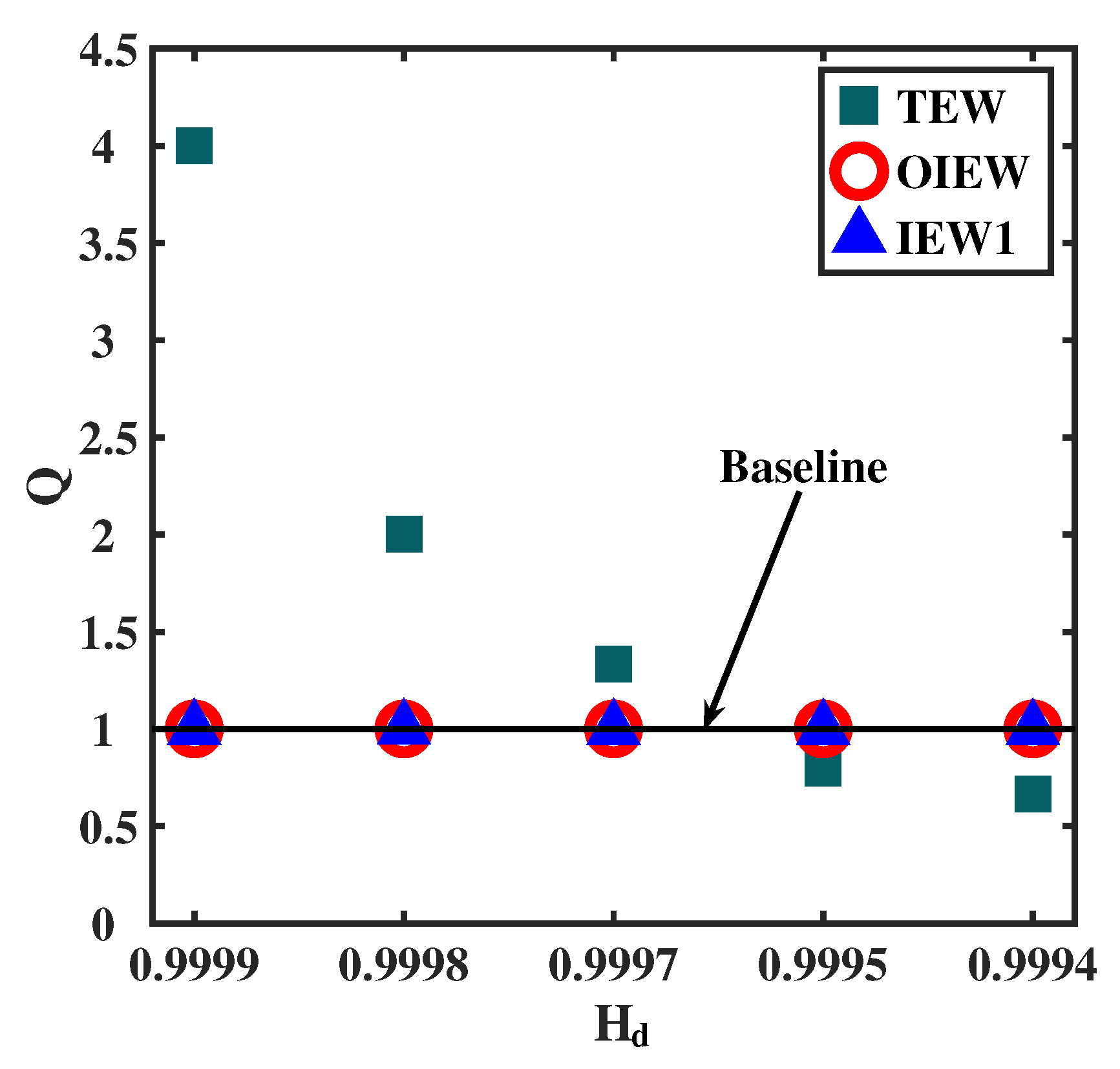
Table 2(a) shows the calculated Q value of TEW method for extreme data. We use 0.9996 as a fixed comparison. It can be observed that the weight ratio
exhibits obviously deviation from 1 when the
is 0.9999, and the Q value is notably lower than 1 when
is 0.9994. The difference in IEV is negligible, whereas the deviation of Q value from 1 is significant. These results further substantiate the inadequacy of the TEW method in weight calculation for extreme data.
To effectively solve this problem, the correct factor is used in TEW method [
12,
14,
18]. Using the IEW1 method, as mentioned in the literature [
18], we demonstrate the limitations of IEW method. The green section in
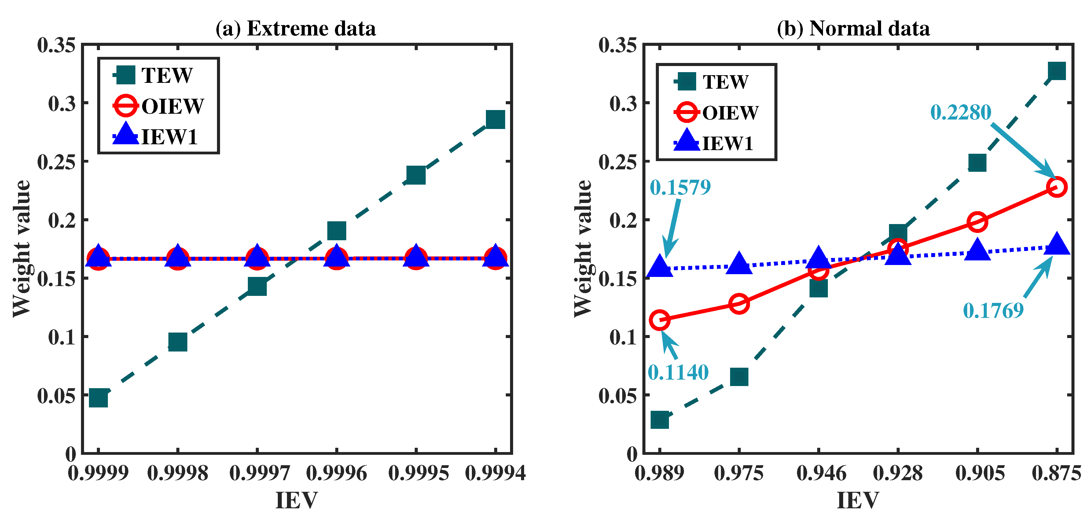
Table 1(b) shows the influence of correction factor for normal data (where larger differences are observed among the IEV). It can be observed that the corresponding weights are 0.1579 and 0.1769 when
is at 0.9890 and 0.8750, respectively. There is a significant disparity in
, but the change in weight remains inconspicuous. The weight changes are smooth when the formula incorporating correction factor. To elucidate this phenomenon, we give the formula [
18] of correction factor, as shown in follows
where
refers the
i-th weight calculated by IEW1 method. The average value
is the correct factor. It can be observed that the increase of the
results in an increment of the numerator. For the extreme data, this increment in the numerator will increase the integer part of the weight value while diminishing the influence of the decimal portion. Ignoring the effect of the fractional part will mitigate the deviation of Q from 1. Therefore, this correction approach can reduces the differences between weights and improves the resistance to extreme data. The green section in
Table 2(b) shows the calculated
Q value of IEW1 method for extreme data. It can be seen that a small fluctuation in the IEV results in a correspondingly minor deviation of the Q value from 1. This phenomenon demonstrates that the addition of correction factors can improve the resistance to extreme data.
However, the integer part also weakens the weight difference of normal data and leads to a larger relative error between the changes in weight values and IEV, as shown in
Table 3. We examine the impact of adding or omitting correction factors on Q values within the same dataset. The TEW method exhibits a clear decreasing trend in Q value as
decreases. However, the introduction of the correction factor
only slightly decrease the
Q value for IEW1 method. Therefore, the correction factor will impact the weight of normal data.
It should be emphasized that we use 1 as the benchmark to measure the degree of deviation between Q and 1 to assess the accuracy of the evaluation method for extreme data, but this benchmark is not applicable to normal data. This is because that there exists a significant disparity between the
and
for normal data (
), thus rendering 1 as a benchmark is inadequate to assess the weight variation. To assess the entropy weight variation of normal data, the
G value is introduced as an evaluative tool for assessing consistency. Equation
4 is formula of
G [
29].
The G value is the standard deviation of the relative error between the differences in adjacent entropy values and those in weights. It denotes the consistency level of the entropy weight variation. A smaller value of
G indicates a higher level of consistency, whereas a larger value of
G signifies that the weights fail to meet the requirement for consistency. According to the calculation formula of standard deviation,
G is a constant value.
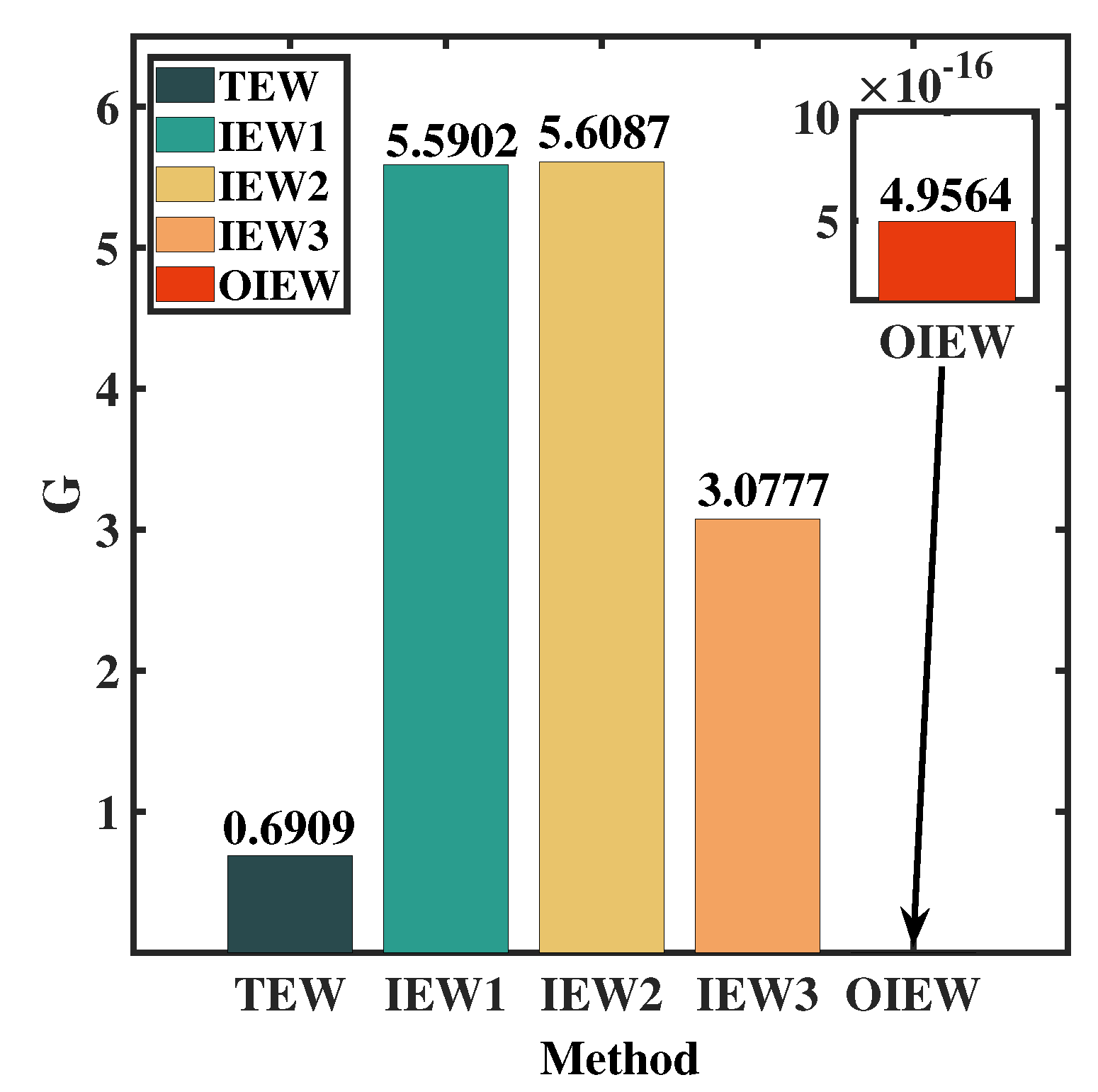
Table 4 shows the G value of different method for normal data and extreme data. It can be observed that the
G value of IEW method is greatly higher than that of the TEW method. These results prove that the consistency of the TEW method is superior for normal data. But, the correction factor used in the IEW method overcompensates for normal data weights, leading to a violation of consistency principle.
Therefore, building an appropriate evaluation model is a pressing issue, which should not only optimize the correction factors to normal data but also enhance the anti-interference ability to extreme data. Moreover, the evaluation process must adhere to the principle of consistency in entropy weight variation.
4. Theoretical model construction
To enhance the robustness to extreme data and mitigate excessive correction in IEW method, we propose an optimized improved entropy weight (OIEW) method to improve the weight determination process. By utilizing linear programming methodology and adhering to the principle of consistency in entropy weight variation, a programming model is constructed to calculate the weight. Furthermore, the FCE method is introduced to the OIEW method to overcome the simplistic of SFE method and provides a comprehensive evaluation for multi-factors systems.
4.1. Construction of evaluation datasets and reference sets, as well as the determination of membership functions
Appropriate sets of evaluation criteria, datasets, and membership functions can effectively reflect the true condition of the evaluated objects and enhance the accuracy of the evaluation results. The detailed construction process see Appendix B and Appendix C.
4.2. OIEW method
The TEW method employs a single formula for weight calculation, which results in insufficient robustness against extreme data. Although correction factors can be applied to each factor, they still rely on a static weight calculation formula. As entropy variation is a dynamic process, it is necessary to use a dynamic solution method that adjusts weight calculations accordingly. Therefore, we transform the mathematical planning model into linear programming model by simplex algorithm.
The weights calculated using the correction factor have a significant impact on normal data. Therefore, we introduce the concept of linear programming and optimize the computation process by imposing specific constraints on each weight. As
G value can effectively characterize the consistency of entropy weight variation, we select it as the objective function in our linear programming model. According to the Equation
4, it can be observed that the smaller the value of
results in a lower
G value, thereby increasing the consistency. Therefore, we construct the objective function
Z, which is defined as
and represent the generalized weight value and IEV, respectively. When the constraints are satisfied, a smaller value of Z indicates more precise weights. The constraints of the objective function are specified as follows: (1) The total weight of all factors is 1; (2) The changes in weights are inversely proportional to the changes in IEV; (3) The weights should range from 0 to 1.
To facilitate comparison with the TEW and IEW methods, we replace
with
to denote the weights calculation in the OIEW method. Therefore, the formula of the OIEW model can be derived by synthesizing the aforementioned concepts.
By utilizing Equation
6 to calculate the weights, maximum consistency with the trend of information entropy changes can be ensured. To achieve stable data acquisition and simplify the calculation process, the single objective function problem is transformed into a linear programming model to optimize the weight calculation process (see Appendix D for the detailed description). The linear programming model that undergoes transformation is formulated as
Where , represent two variables that characterize . Where and represent two variables that characterize .
This linear programming model can be solved by the simplex method. Therefore, to achieve the optimal solution, we must first convert the inequality in formula
7 into the standard form of constraints, resulting in the following equation.
Where is relaxation variables. By introducing this relaxation variables, the inequality constraints of the linear programming problem can be transformed into equality constraints. Then, the optimal solution can be obtained through the simplex method. And, the weights calculated by the dynamic solution process of the simplex method can greatly comply with the principle of consistency in entropy weight variation.
4.3. OIEFC method
The evaluation of multi-factors system by SFE method lacks comprehensiveness. Therefore, we incorporate the FCE method into the OIEW method to establish a multi-factors evaluation model (we call it the OIEFC evaluation model). In this method, the multi-factor set is divided into multiple sub-factor sets, and the first-level FCE is conducted for each subset. Subsequently, the obtained first-level evaluation vectors are further utilized as a new factor set to conduct second-level FCE. By repeating the aforementioned process, it is feasible to carry out comprehensive evaluations at third, fourth, and even higher levels in order to obtain the final evaluation results. This evaluation method fully considers the interrelationships among factors, and the hierarchical processing enhances the significance of weights to yield more accurate evaluation results. In order to further enhance the comprehension of the evaluation process, we present the two-level FCE models an illustrative example. The two-level model include first and second evaluation level.
(1) Establish the second-level FCE matrix.
After obtaining the weight judgment matrix and the weight vector, the FCE matrix can be constructed (The weight judgment matrix obtained is presented in Appendix C). The comprehensive result at the current level are determined by fuzzy algorithm. The final evaluation results can be obtained through step-by-step calculations. The detailed method is as follows:
The FCE matrix is calculated based on fuzzy operations. According to weights formula and simplex algorithm, the FCE matrix of the second-level
can be expressed as
Where p is p-th first level indicator, k is k-th second level indicator. , and are the weight vector, and weight judgment matrix of the second-level factors corresponding to the p-th first-level indicator, respectively. is the weight of the k-th secondary indicator corresponding to the p-th first-level indicator. (where =1,2, …,j) represents the overall membership of the level corresponding to the p-th first-level indicator.
(2) Establish the first-level FCE matrix.
Then, the FCE matrix of second-level factors are taken as the weight judgment matrix of the first-level factors. And the membership of the corresponding first-level factor is determined by the comprehensive membership degree of the secondary factors. Therefore, the weight judgment matrix of the first-level factors
U can be written as
Where
U is the weight judgment matrix of the first-level indicators.
is the
-level membership of the
p-th first-level indicator. By utilizing the weights of the second-level factors as raw data and applying the OIEW method, we can derive the weights of the first-level factors. Then, the FCE matrix of the first-level factors can be constructed. Ultimately, the evaluation of these indicators can be assessed by the principle of maximum membership degree. The evaluation model can be expressed as
Where L is the first-level FCE matrix. is the weights matrix of first level indicator, is the weights of p -th first level indicator. is overall membership of p-th first level. If , the level results of the environmental system are level .
Author Contributions
Conceptualization, M.Z.Y. and Y.X.W.; methodology, M.Z.Y.; software, Y.X.W.; validation, M.Z.Y., Y.X.W. and J.W.; formal analysis, M.Z.Y.; investigation, Y.G.; resources, J.J.S.; data curation, Z.G.W.; writing—original draft preparation, F.B.G.; writing—review and editing,M.Z.Y, Y.X.W. and J.W.; visualization, M.Z.Y.; supervision, J.W.; project administration, J.W.; funding acquisition, S.H.L. All authors have read and agreed to the published version of the manuscript.
Appendix A: Calculation process of TEW method
The weight calculation using TEW method is outlined as follows:
(1) Construct the raw data matrix
Y Suppose there are
n evaluation indicators and
evaluation factors. The raw data matrix
Y can be expressed as
Where is the j-th raw data of i-th evaluate indicator.
(2) Normalization of raw data To mitigate the impact of the original data dimension, we normalized the raw data. The normalization process is as follows
Where is normalized factor values.
(3) Calculate the entropy value of each factor The information entropy value (IEV) of each indicators can be defined as follows
Where is information entropy of i-th indicator. Considering the possibility of zero values in some original data, errors may occur during entropy calculation. To solve this problem, a small increment is added to the indicator value. (e.g. ). This small value can prevent errors while preserving the integrity of the original data.
(4) Calculation of indicator weights
The weights assigned to each indicator can be determined upon completion of the IEV calculation.
Where represents the weights of i-th indicator, and ,
Appendix B: Evaluation Data Set and evaluation criteria set Construction
The evaluation data set is a raw data matrix. The evaluation criteria for each indicator are included in the evaluation set, which is consistently divided into five levels. However, different from the conventional FCE method, each indicator adheres to a strict ranking standard. Thus, this paper utilizes national standards and ranks each evaluation factor in the form of intervals
Where F is evaluation set, represent five levels: I (excellent), II (good), III (moderate), IV (poor), and V (extremely poor). , represent the -th rank and the upper and lower limits of the interval corresponding to the k-th indicator, respectively.
Appendix C: Membership determination
The membership can be determined by the membership function, which is dependent upon the evaluation level value of the evaluation set. The evaluation set is expressed in the form of intervals. Therefore, the membership function is established based on the correlation between factor values and various levels. To facilitate the representation of the membership function, it is advisable to arrange all rank intervals in descending order when considering the irregular arrangement of each rank interval. Ultimately, reverting to the original order after calculating the membership. Membership function are expressed as follow (1)
Where is variable. is the membership of the p-th first indicator corresponding to the k-th secondary indicator at level a. and are the upper and lower limits of the h levels preceding level a for the k-th secondary indicator, respectively. and are the upper and lower limits of the g levels following level level a for the k-th secondary indicator, respectively.
Appendix D: Linearization of nonlinear programming problems
For certain nonlinear programming problems, it can be reformulated as linear programming problems to facilitate the solution process and ensure stable results. For instance, the following equation shows a nonlinear process
where
is the matrices of the corresponding dimensions.
A and
b are vectors.
To convert the aforementioned issue into a linear programming problem, it is simply necessary to take note of the following fact when
and
equal and bigger than 0.
Therefore, we can get
,
. By writing
,
, the aforementioned issue can be transformed into an equivalent form
Here indicates that each component of the vector u is greater than or equal to 0.
Combining the above linearization conversion methods, we can substitute the subsequent variables for Equation
7.
where
,
are the entropy values of the
i-th known metric and its neighbors.
and
are the corresponding weight.
Introducing two new variables
,
converts
and
equivalently, we can obtain
Therefore, by utilizing the Equation D.4 and Equation D.5, we can linearize the weight difference between adjacent indicators to derive the relationship of new various, that is . However, since the constraints are imposed on each weight rather than the difference of the weights, and introducing new variables to represent separate weights would increase complexity, remains a variable in our model.
Bring the aforementioned equation into Equation
7, the linear programming model after variable substitution can be obtained
Figure 1.
Weight comparison among different methods for extreme data (a) and normal data (b). IEV is the information entropy value. TEW, IEW1 and OIEW denote the traditional entropy weight method, the improved entropy weight method and the optimized improved entropy weight method, respectively. The blue numbers are the weight values corresponding to the information entropy.
Figure 2.
Q values of extreme data. is d-th information entropy value. The black baseline line is 1.
Figure 2.
Q values of extreme data. is d-th information entropy value. The black baseline line is 1.
Figure 3.
G values of normal data calculated by different EW methods.
Figure 3.
G values of normal data calculated by different EW methods.
Figure 4.
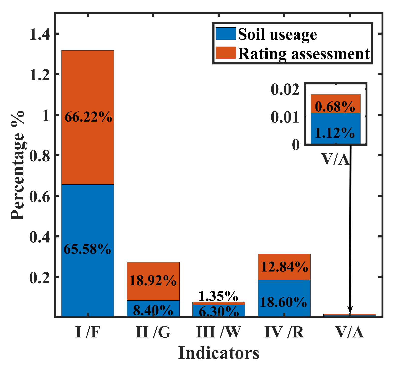
Soil evaluation results and soil utilization percentage. The orange bars are the evaluation grades. The blue bars represent land use types obtained from Shandong Province of Chinese Soil Database, including farmland (F), grassland (G), woodland (W), residential areas (R), and abandoned land (A). The soil evaluation results are divided into five levels: I (excellent), II (good), III (moderate), IV (poor), and V (extremely poor).
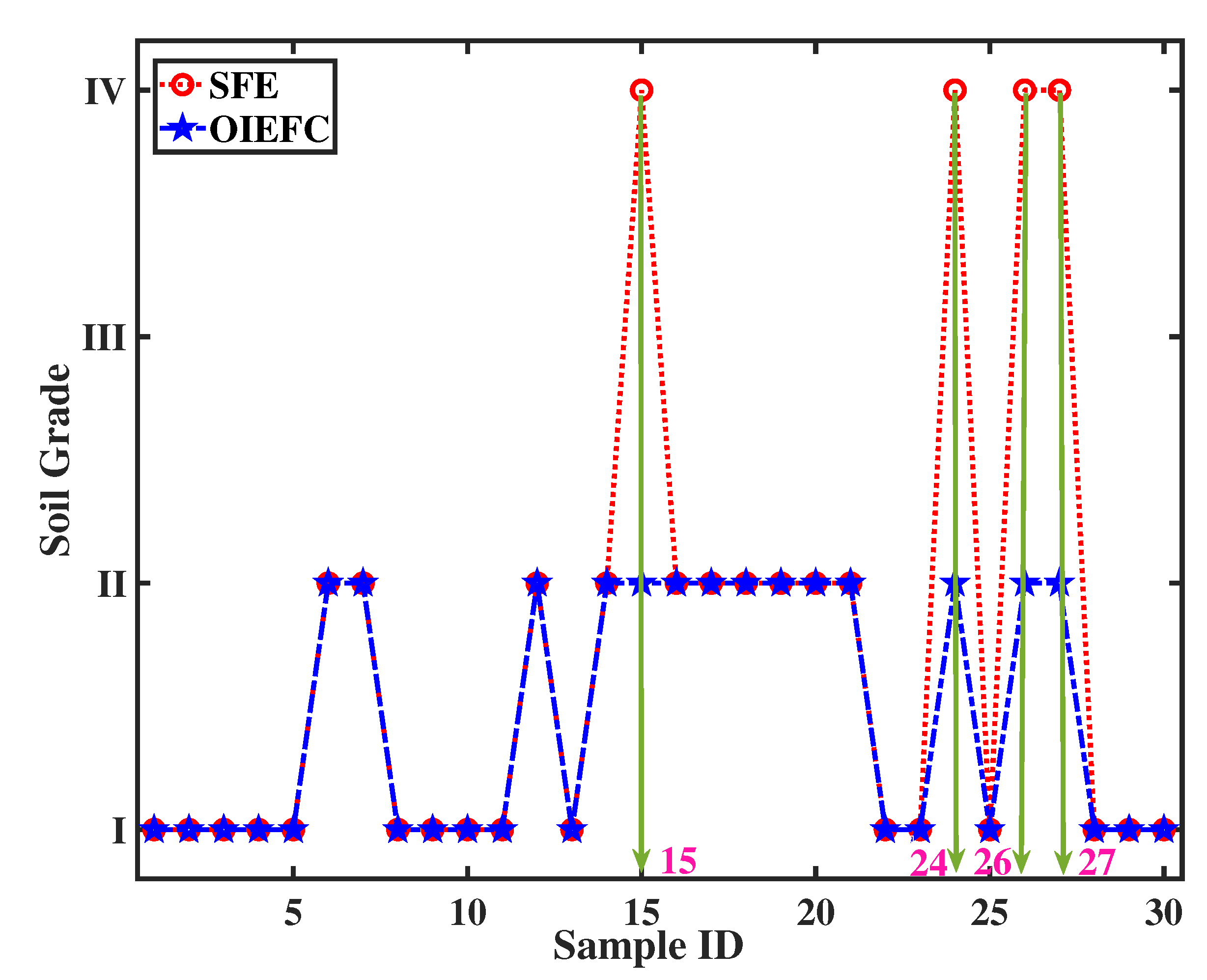
Figure 5.
Comparison of evaluation results between SFE and OIEFC method. Sample ID is the serial number of the soil data. The blue dotted line and the red dashed line are the evaluation results calculated by the SFE method and OIEFC method, respectively. The magenta numbers indicate the serial numbers of the differential evaluation results.
Table 1.
Weights of TEW method and IEW method. represents the i-th information entropy value (IEV). and are the weight calculated by the TEW method and IEW1 method, respectively.
Table 1.
Weights of TEW method and IEW method. represents the i-th information entropy value (IEV). and are the weight calculated by the TEW method and IEW1 method, respectively.
| Condition |
(a) Extreme data |
(b) Normal data |
|
0.9999 |
0.9998 |
0.9997 |
0.9996 |
0.9995 |
0.9994 |
0.989 |
0.975 |
0.946 |
0.928 |
0.905 |
0.875 |
|
0.0476 |
0.0952 |
0.1429 |
0.1905 |
0.2381 |
0.2857 |
0.0288 |
0.0654 |
0.1414 |
0.1885 |
0.2487 |
0.3272 |
|
0.1666 |
0.1666 |
0.1667 |
0.1667 |
0.1667 |
0.1667 |
0.1579 |
0.1602 |
0.1651 |
0.1681 |
0.1719 |
0.1769 |
Table 2.
Q value of different EW methods for extreme data. The correct factor of IEW1 is approximately 0.99965.
Table 2.
Q value of different EW methods for extreme data. The correct factor of IEW1 is approximately 0.99965.
| Method |
(a) TEW method |
(b) IEW1 method |
|
0.9996 |
0.9996 |
|
0.9999 |
0.9998 |
0.9997 |
0.9995 |
0.9994 |
0.9999 |
0.9998 |
0.9997 |
0.9995 |
0.9994 |
| Q |
4.002 |
2.001 |
1.333 |
0.8001 |
0.6668 |
1.0003 |
1.0002 |
1.0001 |
0.9999 |
0.9998 |
Table 3.
Q value of different EW methods for normal data. The correct factor of IEW1 is 0.9305.
Table 3.
Q value of different EW methods for normal data. The correct factor of IEW1 is 0.9305.
| Method |
(a) TEW method |
(b) IEW1 method |
|
0.928 |
0.928 |
|
0.989 |
0.975 |
0.946 |
0.905 |
0.875 |
0.989 |
0.975 |
0.946 |
0.905 |
0.875 |
| Q |
6.545 |
2.882 |
1.333 |
0.758 |
0.576 |
1.065 |
1.049 |
1.018 |
0.978 |
0.950 |
Table 4.
G value of normal data. IEW1, IEW2 and IEW3 are the improved entropy weight method obtained by the literature [
12,
14,
18].
Table 4.
G value of normal data. IEW1, IEW2 and IEW3 are the improved entropy weight method obtained by the literature [
12,
14,
18].
| Method |
TEW |
IEW1 |
IEW2 |
IEW3 |
| G |
0.6909 |
5.5902 |
5.6087 |
3.0777 |
Table 5.
Evaluation values for the chemical and physical indicators. The chemical indicators include organic carbon (OC), potential of hydrogen (PH), cation exchange capacity (CEC), and electrical conductivity (ECE). The physical indicators include soil texture (TEX) and soil bulk density (BULK). The weight values for each indicator should be discussed separately based on the second-level indicator classification.
| Indicator/Method |
IEV |
TEW |
IEW1 |
OIEW |
Chemical
Indicator
|
OC |
0.9837 |
0.0447 |
0.2313 |
0.1752 |
| PH |
0.9979 |
0.0058 |
0.2278 |
0.161 |
| CEC |
0.9807 |
0.053 |
0.2321 |
0.1782 |
| ECE |
0.6733 |
0.8695 |
0.3089 |
0.4856 |
| Physical |
TEX |
0.8932 |
0.899 |
0.5327 |
0.5474 |
| Indicator |
BULK |
0.988 |
0.101 |
0.4763 |
0.4526 |
Table 6.
Difference of evaluation results between ID15 and ID24. Actual measurement data obtained by HWSD dataset which provides raw physical and chemical indicators data for diverse soil indicators. Soil grade calculation results obtained by SFE and OIEFC method.
Table 6.
Difference of evaluation results between ID15 and ID24. Actual measurement data obtained by HWSD dataset which provides raw physical and chemical indicators data for diverse soil indicators. Soil grade calculation results obtained by SFE and OIEFC method.
| ID |
ID15 |
ID24 |
| Actual measurement data |
Physical
indicator
|
TEX |
12 |
12 |
| BULK |
1.58 |
1.6 |
| |
OC |
0.3 |
0.63 |
Chemical
indicator
|
PH |
7.1 |
6.5 |
| CEC |
7 |
6 |
| ECE |
0.1 |
0.1 |
| Calculation evaluation results |
SFE |
II |
II |
| OIEFC |
IV |
IV |
