Preprint
Article

Comparison of Monocular Visual SLAM and Visual Odometry Methods Applied to 3D Reconstruction

Altmetrics

Downloads

410

Views

69

Comments

0

A peer-reviewed article of this preprint also exists.

Submitted:

05 July 2023

Posted:

07 July 2023

You are already at the latest version

Alerts
Abstract
Pure monocular 3D reconstruction is an ill-posed problem that has attracted the research community's interest due to the affordability and availability of RGB sensors. SLAM, VO, and SFM are disciplines formulated to solve the 3D reconstruction problem and estimate the camera’s ego-motion, so many methods have been proposed. However, most of these methods were not evaluated in large datasets, under various motion patterns, had not been tested under the same metrics, and most of them had not been evaluated following a taxonomy, making their comparison and selection difficult. In this research, we performed a comparison of ten publicly available SLAM and VO methods following a taxonomy, including one method for each category of the primary taxonomy, three machine learning-based methods, and two updates of the best methods, to identify the advantages and limitations of each category of the taxonomy and test if the addition of machine learning or the updates made on those methods improved them significantly. Thus, we evaluated each algorithm under the TUM-Mono benchmark and performed an inferential statistical analysis to identify significative differences through its metrics. Results determined that sparse-direct methods significantly outperformed the rest of the taxonomy, and fusing them with machine learning techniques significantly improves the performance of geometric-based methods from different perspectives.
Keywords: 
Subject: Computer Science and Mathematics  -   Computer Vision and Graphics

1. Introduction

Monocular 3D reconstruction is a challenging ill-posed problem that has been studied in the past three decades to obtain 3D representations of an environment using a sequence of images as the unique source of information for an algorithm. Previously multiple researchers have explored the possibility of addressing this problem by using diverse hardware like radars, lasers, GPS, INS, cameras, and any possible combination. Regarding the camera alternative, it can be combined with active or passive infrared sensors as RGB-D input modalities. It can also be structured as an array of cameras registering the same objects from multiple angles to allow triangulation. Monocular RGB sensors can also be used alone to register a frame sequence from which the algorithm can process a scene from multiple views [1,2]. This last option is known as monocular RBG or monocular pure visual input modality, which can be used in monocular Simultaneous Landing and Mapping (SLAM), Visual Odometry (VO), or Structure from Motion (SFM) to obtain 3D reconstructions of environments and estimate the ego-motion of an agent from such representations. In recent years, the pure monocular input modality has attracted the research community’s attention due to the sensors’ low price and availability in most handheld devices (like smartphones, tablets, and laptops). In this way, monocular SLAM, VO, and SFM systems are not limited by other sensors (like lasers or radars) to work in a limited range and have demonstrated the ability to recover precise trajectories and 3D reconstructions indoors and outdoors.
As mentioned before, SLAM, VO, and SFM are three disciplines that can be used to achieve the goal of 3D reconstruction. SLAM is a discipline that has appeared in the robotics field motivated by the objective of estimating the map of the environment from where the trajectory of a robot can be calculated, which can be used for autonomous navigation, driving, and flying, among others. In the computer vision field, multiple systems have been created to address similar problems: SFM and VO. Structure from motion is specialized in recovering the geometry of an environment, while visual odometry is focused on calculating the trajectory and pose of a moving camera. However, it has been demonstrated that, instead of solving each problem separately, the best results have always been obtained by solving and optimizing both problems at the same time [1,3,4,5]. That is why it is common to find VO methods that include SFM modules to improve their performance and SFM methods that use VO to improve estimation or optimization tasks. For such reasons, in this study, we aim to identify the best monocular RGB methods for 3D reconstruction, so we included methods of these three disciplines that are suitable for recovering 3D reconstructions of the environment.
As an ill-posed problem, pure visual monocular 3D reconstruction has been addressed from multiple perspectives combining various techniques that can be classified following different approaches. One early classification is described in the study of [1] defining the feature-based and appearance-based categories; nevertheless, this approach is unsuitable for covering all the SLAM, VO, and SFM techniques available nowadays in state-of-the-art. A better approach to classify monocular RGB 3D reconstruction systems is the taxonomy described in [6], which considers three classifications covering dense, sparse, direct, indirect, classic, and machine learning proposals. Moreover, in that work, the authors listed 42 methods classified following the proposed extended taxonomy. After a careful reading and analysis of the 42 listed methods, we could identify that many of the existing methods were not adequately evaluated in large datasets [7,8,9,10] or were not tested under different motion patterns and illumination changes [8,11,12], or were not tested for indoors and outdoors [13,14,15]; or the provided results were not obtained on the same metrics [5,16,17], which difficult their comparison and selection. In addition, most of the methods perform comparisons against currently available methods from state of the art, providing results on tables summarizing the average mean or median of the algorithm execution on a specific scene, but they do not provide an inferential statistical analysis of the results; thus, the reported differences or improvements cannot be considered significant. Moreover, given the fact that before the extended taxonomy described in [6] there existed only general classifications like direct vs. indirect and sparse vs. dense methods [1,4,5], or the taxonomy described in [18], none of the studies compared their results following a taxonomy that allows identifying better the advantages and limitations of direct, indirect, dense and sparse methods.
To address the mentioned issues, in this study, we performed a comparison of ten publicly available SLAM and VO methods following a taxonomy, where the main contributions are:
  • A comparison of 10 SLAM and VO methods, following the main classification described in the taxonomy (sparse-indirect, dense-indirect, dense-direct, sparse-direct), to identify the advantages and limitations of each method of those classifications.
  • A comparison of three machine learning-based methods against their classic geometric versions to identify if there exist significative improvements in adding neuronal networks to classic approaches.
  • An inferential statistical analysis that describes a correct procedure to identify significative differences based on the most suitable metrics for testing monocular RGB methods.
We also provide video samples of the execution of each algorithm as supplementary material in the GitHub repository: https://github.com/erickherreraresearch/MonocularPureVisualSLAMComparison, along with all the .txt result files of each algorithm run for reproducibility.

1.1. Related works

An early work that accurately compared monocular visual odometry systems was the study of [19], where authors compared the state-of-the-art methods of that time, DSO, ORB-SLAM, and SVO, on the TUM-mono benchmark. The authors found that the DSO system, even being a visual odometry system, outperformed the SLAM method and the popular SVO. In that study, authors also tested photometric calibration, motion bias, and rolling shutter effect, with the available information provided in the TUM-Mono dataset, finding that the photometric calibration improves the performance of direct methods considerably, and the motion bias effect was more prominent in the indirect method. In contrast, in our study, we compared ten methods following a taxonomy, where the three methods tested in [19] were also addressed, and we explored the same photometric calibration, motion bias, and rolling shutter effects by applying the TUM-Mono dataset. Then in 2020, Mingachev et al. published two comparisons [20,21] testing first DSO, LDSO, and ORB-SLAM2 and then the ROS-Based methods DSO, LDSO, DynaSLAM and ORB-SLAM2 on the TUM-Mono and EuRoC benchmarks. In those studies, authors verified the performance of those algorithms implementing the open-source code in their hardware to determine if there exist improvements on the methods LDSO and DynaSLAM that are updates of the original DSO and ORB-SLAM2. The authors found that the updates achieved slight error reductions over their predecessors on both benchmarks, reported as the average of the medians of 10 algorithm runs in each sequence.
In contrast to those studies, we tested ten methods following a taxonomy to test whether the newer versions improved their previous performance and identify advantages and disadvantages in the entire taxonomy. We also provide a complete inferential statistical analysis of each method’s performance, not only their median values. In addition, we included machine learning-based versions of the classic methods in our comparison. One of the most recent related works is the study of [22] which explored the state-of-the-art classification and tested visual and visual-inertial algorithms in the ERoC benchmark. In that work, the authors made a brief overview of the existing methods and reviewed the classic classification of direct, feature-based, and RGB-D methods. In addition, they implemented the DSO, ORB-SLAM2, and Vins-Mono methods on the EuRoC benchmark. In contrast, this comparison is focused only on monocular RGB methods, so we followed an appropriate taxonomy for monocular RGB SLAM and VO systems. In addition, we used the TUM-Mono benchmark and its metrics, which is a broader and more complete benchmark.

2. Materials and Methods

For this study, we used as materials and methods the taxonomy, algorithms, benchmarks, and metrics suitable for the monocular SLAM and VO problems, which will be discussed in the following sections.

2.1. Taxonomy

The prior work [6] described a taxonomy based on three classifications in the literature: direct vs. indirect, dense vs. sparse, and classic vs. machine learning.
  • Direct vs. indirect. Indirect methods refer to those algorithms that implement preprocessing steps, like feature extraction or optical flow estimation, before their pose and map estimation processes, so the amount of information that gets into the following steps gets considerably reduced, requiring less computational power but also reducing the density of the final 3D reconstruction. Indirect methods typically perform their optimization steps by minimizing the reprojection error due to the feature type of information that the preprocessing step outputs. On the other hand, direct methods work directly on pixel intensity information without requiring preprocessing steps, which implies that the algorithm has more information available for their estimation tasks, being available to obtain denser reconstructions of the scene but requiring more computational power. In addition, direct methods typically perform their optimization steps based on the photometric error due to the availability of direct pixel information.
  • Dense vs. sparse. Dense vs. sparse classification refers to the amount of information recovered in the final map as a 3D reconstruction. Denser reconstructions have more definition and continuity in the reconstructed objects and surfaces. In contrast, sparser reconstructions are typically represented as point clouds largely separated where edges and corners are commonly the only types of objects that can be recognized clearly.
  • Classic vs. machine learning. Classic methods have been proposed in the last three decades, typically basing their formulation on geometric, optimization, and probabilistic techniques without machine learning. However, in recent years, due to the impressive advances in artificial intelligence, especially in Convolutional Neural Networks (CNN), many techniques have been applied to improve SLAM or VO estimation tasks. The methods based on classic formulations and improved with machine learning are called Machine Learning based approaches (ML).
Combining these three classifications in all their possible configurations [6] establishes the taxonomy: classic + dense + direct, classic + sparse + direct, classic + dense + indirect, classic + sparse + indirect, classic + hybrid, ml + dense + direct, ml + sparse + direct, ml + dense + indirect, ml + classic + sparse + indirect and ml + hybrid. It must be mentioned that the hybrid category was added for those methods that efficiently combine the direct and indirect principles to estimate the pose and scene geometry, like SVO [10] and CNN-SVO [8]. Figure 1 depicts the monocular RGB taxonomy for SLAM, SFM, and VO algorithms.

2.2. Selected algorithms

In this comparative analysis, we pursued to determine the advantages and limitations of the taxonomy classifications and explore as many categories of the taxonomy as possible. For this purpose, we selected and implemented five methods, one for each category of the classic classification. Furthermore, we included three machine-learning versions of the selected classic approaches to test the hypothesis of whether or not the addition of CNN to classic approaches significantly improves the performance of geometric-based methods. In the prior work [6], many machine learning approaches were listed, which are available as open-source code [14,16,23,24,25,26,27,28,29,30,31,32,33,34]. However, during their implementation, we found that many implementations are available for multiple input modalities like RBD-D or INS. However, the provided code was not available for monocular RGB as the unique input source of information, or they required external modules to work, which was not included; thus, we could not include those methods for this comparison, e.g., [25,30,33,34]. Finally, we added two additional sparse-direct implementations built over the DSO [18] system, given the impressive 3D reconstruction results that this method demonstrated during evaluations.
In this way, the algorithms selected to perform this comparative study were:
  • ORB-SLAM2. As a sparse-indirect representant, we selected ORB-SLAM2 [35], which is widely known as the gold standard of this category, as most of the currently available sparse-indirect methods are proposals inspired by this algorithm. Original ORB-SLAM [36] extracts ORB features as preprocessing that are multiscale FAST corners with a 256-bit descriptor, which gives that algorithm information to perform a Bundle Adjustment for optimization and work in three threads for tracking, local mapping, and loop closure. In addition, ORB-SLAM2 incorporates a fourth thread to perform a full Bundle Adjustment after loop closure, which is demonstrated to improve the original method allowing it to obtain the optimal geometric representation of the scene. ORB-SLAM2 is publicly available as open source code in [37]; it can be implemented in its C++ version or ROS version, with minimum additional requirements, which are Pangolin, OpenCV (tested for 2.4.3 version), Eigen 3 (tested for 3.1.0 version), DBoW2 and g2o which are included in the repository.
  • DF-ORB-SLAM. Classic-dense-indirect methods available in the literature, like [38,39], are not available as open-source code for implementations, so they could not be considered for this evaluation. Instead, a well-known classic-dense-direct version of ORB-SLAM2 exists, called DF-ORB-SLAM [13], with its code publicly available on GitHub. DF-ORB-SLAM algorithm was built based on the ORB-SLAM2 algorithm, allowing the addition of depth map retrieval capabilities and incorporating optical flow to track the detected points; thus, this algorithm uses a large amount of information obtained through the input using most of the pixel values for optical flow estimation. Once the optical flow is estimated, ORB-SLAM2 performs feature extraction on the optical flow domain and executes the rest of its pipeline. DF-ORB-SLAM is publicly available in [13], and it was implemented in Ubuntu 18.04 in its ROS version using its official build_ros.sh script.
  • LSD-SLAM. LSD-SLAM [40] is one the most popular methods of the dense direct category since it has been the basis and inspiration of a lot of the methods currently available [7,18,41]. LSD-SLAM not only locally tracks the camera’s movement but also allows the construction of dense maps of the environment through a semi-dense geometric representation, which tracks depth values only in high-gradient areas. The method has direct image alignment mechanisms and estimation based on the semi-dense depth map filtering technique [42]. The global depth map is rendered as a pose graph comprising keyframes represented as vertices that present feature 3D similarity transformations as edges, adding environment scaling ability and allowing accumulated drift to be detected and corrected. Furthermore, LSD-SLAM uses an appearance-based loop detection algorithm called FAB-MAP [43], which proposes prominent loop closure candidates that extract their features without reusing any additional visual odometry information. LSD-SLAM is publicly available in [44] and was implemented in Ubuntu 18.04 in its ROS version.
  • DSO. DSO [18] is considered widely known as the gold standard of direct methods due to the impressive reconstruction and odometry results that it has achieved, and it has inspired and kept inspiring many implementations and new proposals. DSO works directly on pixel intensities information but applies a point selection strategy to reduce the amount of information to be processed efficiently. It continuously optimizes photometric error applied to the last N-frames while optimizes the complete likelihood for all the parameters involved in the model, including poses, intrinsics, extrinsics, and inverse depths, executing a windowed sparse bundle adjustment for this. DSO is publicly available for implementation in [45], and its code runs totally in C++ using minor requirements like Suitesparse, Eigen3, and Pangolin.
  • SVO. We selected the most commonly known method, SVO [9], for the hybrid classification. SVO efficiently combines the advantages of direct and indirect approaches by using feature correspondences obtained on direct motion estimation for tracking and mapping. This procedure considerably reduces the number of required features and is only executed when a new keyframe is selected to insert new points in the map. First, camera motion is estimated by a sparse model-based image alignment algorithm, where sparse point features are used to estimate feature correspondences. Next, this information is used to minimize the photometric error. Then reprojected points, pose, and structure are refined by minimizing the reprojection error. SVO is publicly available in [46] for testing and implementation and runs on C++ or ROS. Modern operating systems might find issues during implementation, so Ubuntu 16.04 and ROS kinetic were used for its implementation.
  • LDSO. As an additional sparse direct system, we selected LDSO [47], an update of the DSO algorithm that includes loop closure capabilities. LDSO enables the DSO framework to detect loop closure by ensuring point repeatability using corner features to detect loop candidates. For this purpose, the depth estimates for those point features allow the algorithm to compute Sim(3) constraints, to be combined with pose-only bundle adjustment and point cloud alignment to be fused with the relative pose co-visibility graph of the DSO sliding window optimization stage. This way, LDSO adds loop closure to the DSO system, including a loop closure module based on a global pose graph optimization that works over the last 5 to 7 keyframes sliding window. LDSO was made publicly available in [48], and for this comparison, it was implemented in Ubuntu 18.04 along with OpenCV 2.4.3, Sophus, DBoW3, and g2o.
  • DSM. Another sparse-direct method we were interested in testing was DSM [49], another update made over DSO to create a complete SLAM system. DSM aimed to include scene reobservation information to enhance precision and reduce drift and inconsistencies. In contrast to LDSO, which considers a sparse set of reobservations, DSM builds a persistent map that allows the algorithm to reuse existing information by a photometric formulation. DSM uses local map co-visibility window criteria to detect the active keyframes reobserving the same region, a coarse-to-fine strategy to process that point reobservation information, and a robust nonlinear photometric bundle adjustment technique based on photometric error for outlier detection. DSM open-source code is publicly available in [50], and it was implemented for comparisons on Ubuntu 18.04 with Eigen (v3.1.0), OpenCV (v2.4.3), and the Ceres solver provided in its official repository.
  • DynaSLAM. Dyna-SLAM algorithm [51] was made over a lighter version of ORB-SLAM2 and was improved by adding ML capabilities for detection, segmentation, and inpainting of dynamic information on scenes. In addition, the Mask R-CNN of [52] was integrated with the classic sparse-indirect method to detect and segment regions of each image that potentially belong to movable objects. The authors also incorporated a multi-view geometry approach that calculates back-projections of each key point to compute parallax angles, which are then used to detect additional dynamic information that the CNN cannot recognize. Authors reported that this combination contributes to overcoming initialization issues of ORB-SLAM2 and allows it to work in dynamic environments. DynaSLAM is publicly available in [14], and it was implemented in Ubuntu 16.04 with ROS Kinetic, Cuda 9, Tensorflow 1.4.0, and Keras 2.0.8.
  • CNN-DSO. In the literature can be found neuronal versions of the DSO method like D3VO [53], MonoRec [11], and DDSO [54]. Nevertheless, they are not publicly available, or in the case of MonoRec, its monocular VO pipeline is not available for testing, so we chose CNN-DSO for this comparison which is publicly available in [12]. This method includes a CNN depth prediction module that enables the DSO system to execute its estimation modules using additional depth prior information obtained by the network. The CNN used for this study was the MonoDepth system of [55], a single image depth estimation network that outputs a depth value for each pixel position by chains of feature maps processing. The network was built over the ResNet backbone using a variant of its encoder-decoder architecture. CNN-DSO requires building TensorFlow (v1.6.0) from source and MonoDepth from its official repository [56], and it was implemented in Ubuntu 18.04 with Eigen (v3.1.0), OpenCV (v2.4.3).
  • CNN-SVO. In the study of [8], an extension of the hybrid method SVO was proposed by fusing the same Single Image Depth Estimation (SIDE) CNN MonoDepth module used in CNN-DSO with the original geometric-based hybrid method. In this case, MonoDepth was included to add preliminary depth information to the SVO pipeline to reduce uncertainty in the feature correspondence identification steps. In this way, the system is initialized, obtaining maps with high uncertainty. Then the SIDE CNN creates filters to approximate the mean and variance of the current values, considerably reducing the amount of information separating inliers and outliers for the depth map. CNN-SVO is publicly available in [26], and it was implemented in Ubuntu 16.04 to allow SVO modules to work with ROS Kinetic.
For more information on taxonomy, definitions, SLAM, VO, and SFM basics, and further details of the methods described in this review, we encourage the reader to look at the prior works listed in [6].

2.3. Benchmarks

There are several datasets and benchmarks available in the literature for evaluating SLAM, SFM, and VO systems like [3,5,57,58,59,60,61,62,63,64,65]. Nevertheless, only a few are suitable for pure monocular RGB systems due to the nature of image acquisition, the type of camera calibration or camera models employed, and the format of the provided ground truth. In this way, we can mention that among the reviewed available datasets, the following can be applied for monocular algorithms comparison:
  • KITTI. The KITT dataset of [59] contains 21 video sequences of a driving car, where the movement parameters are limited to forward driving. The available images have pre-rectification treatments, and the data set provides a ground truth obtained through an assembly of GPS and INS.
  • EUROC-MAV. The EUROC-MAV dataset of [60] contains 11 inertial stereoscopic sequences of a quadcopter flying in different indoor environments. The data set also provides the ground truth values of all frames and calibration parameters.
  • TUM-Mono. The TUM-Mono dataset of [3] presents 50 sequences of indoor and outdoor environments obtained using monocular RBG cameras on monochrome uEye UI-3241LE-M-GL cameras equipped with Lensagon BM2420 (with 148˚ × 122˚ field of view) and Lensagon BM4018S118 (with 98˚ × 79˚ field of view) sensors. This benchmark includes the photometric calibration parameters of each camera, the ground truth, the timestamps for the execution of each image sequence, and the calibration file for the vignetting effect for each sequence. This dataset comprises more than 190,000 frames and more than 100 minutes of video.
  • ICL-NUIM. The ICL-NUIM benchmark of [5] has eight sequences in conjunction with its ray-tracing of 2 environments. It provides the ground truth values of each sequence and the intrinsics of the cameras, and no photometric calibration is required. This data set presents degenerative and purely rotational motion sequences that are usually especially demanding for monocular algorithms.
As can be noticed, the most complete and largest dataset of the above is the TUM-Mono, which is why we employed this dataset in this comparison study. It also has the advantage of being the only dataset that was obtained purely depending on a monocular RGB setup, without depending on any additional sensor or source of information, which, as mentioned in [3,20,21], makes it ideal for comparing visual only SLAM and VO systems. In addition, this benchmark provides the completest set of metrics that can be explored to efficiently compare the selected algorithms in multiple dimensions, which will be discussed in the following section.

2.4. Metrics

As SLAM, SFM, and VO are ill-posed problems that can be addressed from multiple perspectives and a wide variety of techniques, comparing the final obtained 3D reconstruction is not the best alternative for monocular RGB methods because of the different sparsity, scale, and type of output that each method brings, and due to difficulty of accruing accurate ground truth maps [66]. At the same time, trajectories can be acquired using INS, GPS, LASER, RADAR, LIDAR, and Kinect systems, among others, with acceptable accuracy. In this way, as discussed in [3], the best way of comparing SLAM and Vo algorithms of diverse nature (see Figure 1 and Figure 2) is by comparing the trajectory that each algorithm outputs because, even if the method is focused on reconstruction only, is demonstrated that solving both problems, landing, and mapping, simultaneously brings the best reconstruction results [1], from which the quality of the final reconstruction tightly depends in the quality of ego-motion estimation. This way, the metrics we used for this comparison are entirely based on ego-motion estimation, which can be effectively compared for all SLAM and VO algorithms. Among the different metrics for ego-motion available in the literature, we found that the metrics that are present in most of the methods listed in [6] are: the Absolute Trajectory RMSE (ATE), relative pose RMSE (RPE), the cumulated trajectory, rotation, and scale errors, the alignment error and the alignment RMSE.
ATE and RPE are widely applied along with the EUROC dataset and are local pose accuracy metrics proposed by [66]. The relative pose error is a metric for the accuracy of an estimated trajectory over a defined time interval Δ . In this way, this metric corresponds to the drift of the estimated trajectory. For a sequence of estimated poses P 1 ,     ,   P n   S E ( 3 ) and a ground truth trajectory Q 1 ,     ,   Q n   S E ( 3 ) , the relative pose error for each timestamp i is:
E i   : = ( Q i 1 Q i + Δ ) 1 ( P i 1 P i + Δ )
So, for a sequence of n poses, an m = n Δ number of relative poses is obtained. Then the Root Mean Square Error (RMSE) for such errors over all the timestamps of the sequence can be calculated as:
R M S E ( E i : n ,   Δ )   : = 1 m i = 1 m t r a n s ( E i ) 2
Where t r a n s ( E i ) corresponds to the translational component of the relative pose error E i . Many VO or SLAM systems can be evaluated for a timestep interval Δ = 1 , but there exist methods that work on a frames or keyframes window (like [18,47,50]); thus, different Δ values might be appropriate for testing. So, for the evaluation of SLAM systems, it can also be useful to get the RMSE for all the possible time intervals:
R M S E ( E i : n ) = 1 n Δ = 1 n R M S E ( E i : n , Δ )
On the other hand, ATE is proposed to evaluate the estimated trajectory’s global consistency. ATE estimation was achieved by comparing the absolute distances between the estimated trajectory and the ground truth directly. For this, the trajectories are first aligned using Horn’s method [67] to find the rigid body transformation S , to map the estimated trajectory P 1 : n into the ground truth trajectory Q 1 : n , so the absolute trajectory error for each timestamp i can be calculated as:
F i   : = Q i 1 S P i
In the same way as RPE, the RMSE for all the timestamps of the translational components is calculated as follows:
R M S E ( F i : n )   : = 1 n i = 1 n t r a n s ( F i ) 2
Thus, for the [66] benchmark, it can be noticed that RPE combines both translational and rotational errors elegantly, while ATE considers only the translational error component. In contrast, for the TUM-Mono benchmark [3], authors propose to benefit from large loop sequences. This way, instead of using the complete exploring motion pose information; the TUM-Mono benchmark was built to register the ground truth of each sequence’s first and last 10-20 seconds, using LSD-SLAM [40] method to track only those segments. In this way, authors used the accumulated drift for all their metrics, and they demonstrated that the error registered by each evaluated run is not originated in the drift of the SLAM method used to register the ground truth; instead, it came from the drift accumulated by the algorithm through all the trajectory, so any SLAM or VO system can be used to register the start and end segments ground truth. Consequently, the TUM-Mono benchmark aligns the estimated trajectory with the start and end ground truth segments and measures their differences. Let p 1 ,     ,   p n   3 the estimated tracked positions for the   1 to   n frames, S [ 1 ; n ] and E [ 1 ; n ] the frame indices corresponding to the start- and end-segments for the ground truth positions p ^ 3 . Then, by aligning the estimated trajectory with the ground truth start- and end-segments, two relative transformations can be calculated as:
T s g t   : = argmin T S i m ( 3 ) i S ( T p i p ^ i ) 2
T e g t   : = argmin T S i m ( 3 ) i E ( T p i p ^ i ) 2
By these transformations, the accumulated drift can be calculated as:
T d r i f t   : = T e g t   ( T e g t ) 1
The translation, rotation, and scale error components can be extracted as:
e t   : =   t r a n s l a t i o n ( T d r i f t ) e r   : =   r o t a t i o n ( T d r i f t ) e s   : =   s c a l e ( T d r i f t )
In this way, authors established the alignment error, which is a metric that equally takes into account the errors produced by the translational, rotational, and scale effects:
e a l i g n   : =   1 n i = 1 n T s g t p i T e g t p i 2 2
This metric can be computed individually for the star- and end-segment, but when it is estimated by combining both intervals, it is equivalent to the translational RMSE when aligned to the ground truth. Thus, it can also be formulated as follows:
e r m s e   : =   min T S i m ( 3 ) 1 | S E | i S E ( T p i p ^ i ) 2
As it can be observed, in contrast to APE and ATE, that only include two metrics explaining rotation and translation effects, the TUM-Mono benchmark allows to analyze of the performance of a SLAM or VO method in a more detailed way, providing six metrics to explain the amount of accumulated translation, rotation and scale errors, as well as determining the performance of the algorithm in the start- and end-segment to better identify initialization and accumulated drift errors, which finally allows calculating the translational RMSE to visualize global effects of the combined metrics on the whole evaluated sequence. For these reasons, we selected the TUM-Mono and its official metrics to execute this comparison in a complete manner.

3. Results

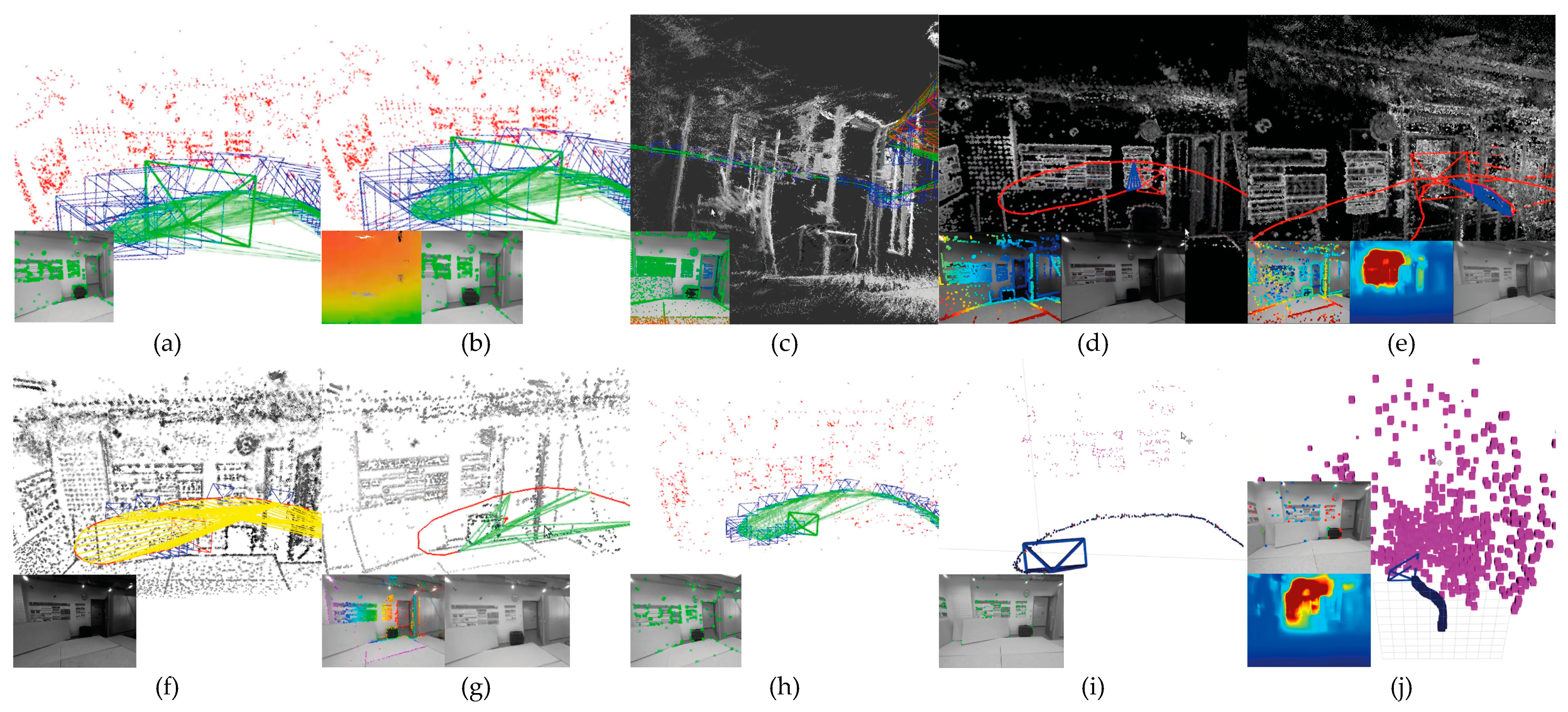
As mentioned above, algorithms were selected based on their open-source availability and independency from any additional input information source other than a monocular RGB frame sequence. Following the primary taxonomy described in [6,18], we selected the classic-sparse-indirect system ORB-SLAM2 [35], the classic-dense-indirect system DF-ORB-SLAM [13], the classic-dense-direct system LDS-SLAM [40] and the classic-sparse-direct method DSO [18]. Then, we added to this study the currently available ML implementations of ORB-SLAM2 [35], DSO [18], and SVO [10], which are DynaSLAM [51], CNN-DSO [12] and CNN-SVO [8]. In addition, we included additional direct proposals derived from the DSO system due to the impressive reconstruction results that this method shown in during experimental evaluation; thus, we selected the LDSO [47] and DSM [49] systems representing the addition of loop closure and SLAM capabilities for DSO system. Figure 2 and Figure 3 present some examples of the execution of the evaluated algorithms on outdoor and indoor sequences of the TUM-Mono dataset.

3.1. Hardware Setup

All methods were evaluated on the same hardware platform with the same available computational and power resources using Ubuntu 18.04 and 16.04 operating systems, depending on the software requirements of each algorithm. For this evaluation, we selected readily available and cheap hardware components to assemble a desktop based on the AMD Ryzen™ 7 3800X processor and the GPU NVIDIA GEFORCE GTX 1080 Ti. Technical specifications are summarized in Table 1.

3.2. Comparative analysis

As addressed in related works [3,35], authors suggest running five times each sequence of a benchmark to create cumulative-error plots and account non-deterministic nature of each system [21]. Nevertheless, authors like [47,51] performed their experimental comparisons by running each sequence ten times in forward and backward reproduction directions to better capture the probabilistic behavior of the algorithms against multiple variations like illumination and dynamic objects. In this way, we applied this extended approach, given the large variety of algorithms we tested. In total, we performed ten runs of each of the 50 sequences in forward and backward modalities, gathering a total of 1000 runs for each method, so for the ten evaluated algorithms, we created a database of 10000 trajectory files saved in .txt format that were processed using the MATLAB scripts provided in the official repository of the TUM-Mono benchmark [3]. Each algorithm must output a file where each P i pose for the trajectory must be in the format represented in equation 1, which has to match the benchmark evaluation scripts format. However, some algorithms like SVO, CNN-SVO, and DSM outputs rotation and translation matrixes instead of quaternions, so we modified those algorithms to bring the correct output format using the proposal of Sarabandi and Thomas [68] by equations 2, 3, 4, and 5.
P i = ( t i     x i     y i     z i     q x i     q y i     q z i     q w i )
Given the rotation matrix:
R = ( r 11 r 12 r 13 r 21 r 22 r 23 r 31 r 32 r 33 )
q x = { 1 2 1 + r 11 + r 22 + r 33 , i f   r 11 + r 22 + r 33 > η 1 2 ( r 32 r 23 ) 2 + ( r 13 r 31 ) 2 + ( r 21 r 12 ) 2 3 r 11 r 22 r 33 , o t h e r w i s e
q y = { 1 2 1 + r 11 r 22 r 33 , i f   r 11 r 22 r 33 > η 1 2 ( r 32 r 23 ) 2 + ( r 12 + r 21 ) 2 + ( r 31 + r 13 ) 2 3 r 11 + r 22 + r 33 , o t h e r w i s e
q z = { 1 2 1 r 11 + r 22 r 33 , i f r 11 + r 22 r 33 > η 1 2 ( r 13 r 31 ) 2 + ( r 12 + r 21 ) 2 + ( r 23 + r 32 ) 2 3 + r 11 r 22 + r 33 , o t h e r w i s e
q z = { 1 2 1 r 11 r 22 + r 33 , i f r 11 r 22 + r 33 > η 1 2 ( r 21 r 12 ) 2 + ( r 31 + r 13 ) 2 + ( r 32 + r 23 ) 2 3 + r 11 + r 22 r 33 , o t h e r w i s e
As reported in [68], the best results that outperform Shepperd’s rotation to quaternion method are achieved for η = 0 , so we set this value to build the trajectory files for those methods that did not match the evaluation format. In addition, methods ORB-SLAM2, DF-ORB-SLAM, DynaSLAM, SVO, CNN-SVO, and DSM require a different calibration camera model than the provided by the benchmark that includes full photometric data considering geometric intrinsic calibration, photometric calibration, and non-parametric vignette calibration. In this way, while the rest of the methods use the ATAN camera model based on the FOV distortion model of [69] provided in the official PTAM repository [70], we used the ROS calibration package [71] to estimate three radial and two tangential distortion coefficients d c o e f f = ( k 1     k 2     p 1     p 2     k 3 ) which follows the formulation of equations 6 and 7, and the results were also tested and compared with the OpenCV Camera calibration package [72].
For each pixel undistorted pixel at ( x u , y u ) coordinates, its position in the distorted image is ( x d , y d ) :
x u = x d ( 1 + k 1 r 2 + k 2 r 4 + k 3 r 6 ) y u = y d ( 1 + k 1 r 2 + k 2 r 4 + k 3 r 6 )
x u = x d + [ 2 p 1 x d y d + p 2 ( r 2 + 2 x d 2 ) ] y u = y d + [ p 1 ( r 2 + 2 y d 2 ) + 2 p 2 x d y d ]
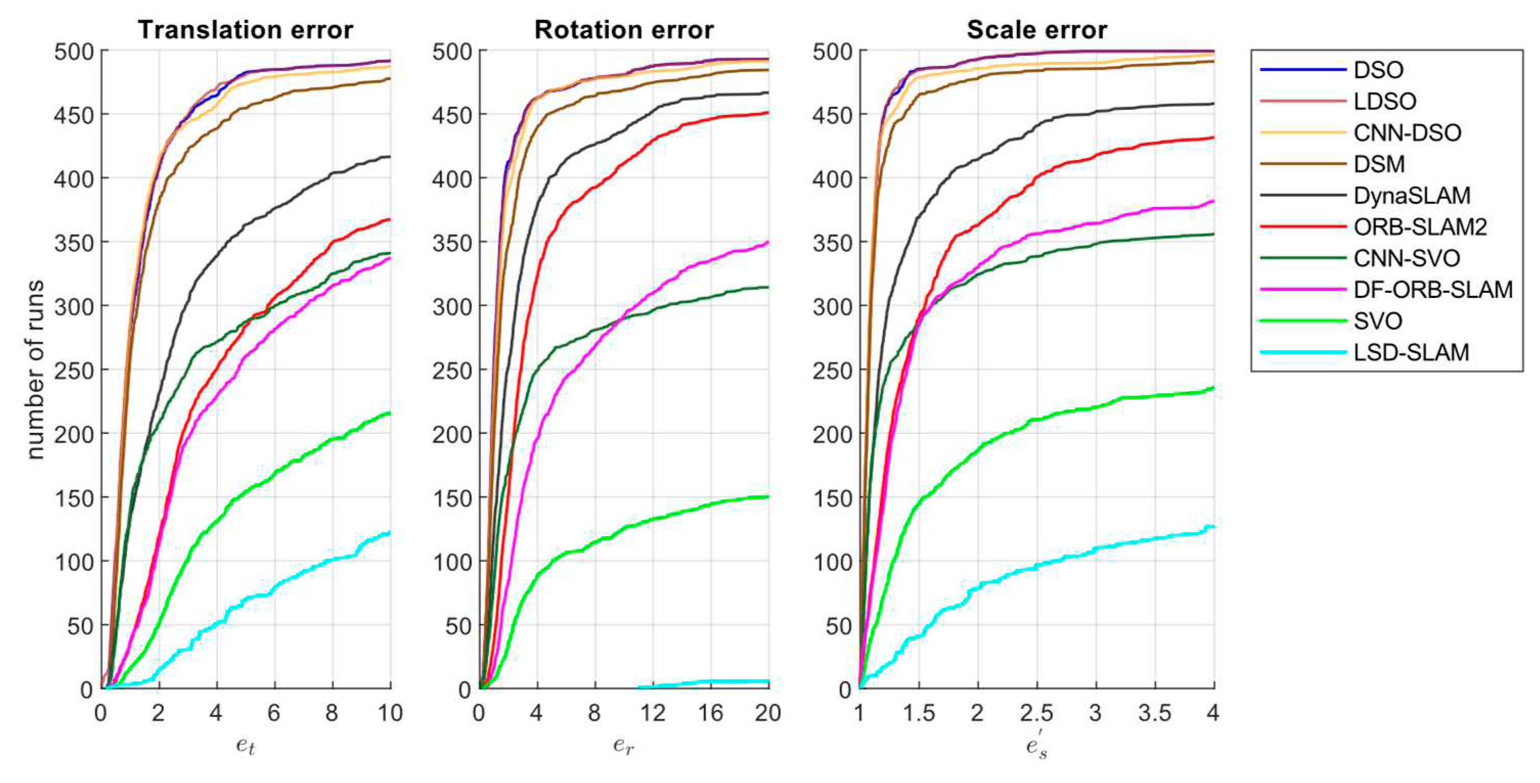
Where r is the distorted radius r d = x d 2 + y d 2 . As suggested in [3], to make a fair comparison based on the accumulated drift over the aligned start and end sequences, we disabled loop closure for the SLAM methods ORB-SLAM2, DF-ORB-SLAM, DynaSLAM, LDSO, and DSM. Figure 4 presents each algorithm’s cumulative error plots for the translational, rotational, and scale errors. These graphs depict the number of runs for each error type below a certain x-value. Hence, methods close to the top left corner are better because they reach a determined error value after more executions.
As can be seen in Figure 4, sparse direct methods (DSO, LDSO, and DSM) achieved the best overall performance, followed by the sparse indirect method (ORB-SLAM2), the dense indirect method (DF-ORB-SLAM), the hybrid method (SVO) and the dense direct method (LDS-SLAM) shown the worst performance. CNN versions of ORB-SLAM2 and SVO showed an important improvement over their classic versions. At the same time, CNN-DSO did not outperform DSO in accumulated translation, rotation, and scale metrics but kept close to the performance of DSO. Finally, it must be mentioned that the large error observed in LSD-SLAM, SVO, and CNN-SVO methods can be attributed to severe initialization and relocalization problems that the algorithms presented during evaluations in the TUM-mono dataset.
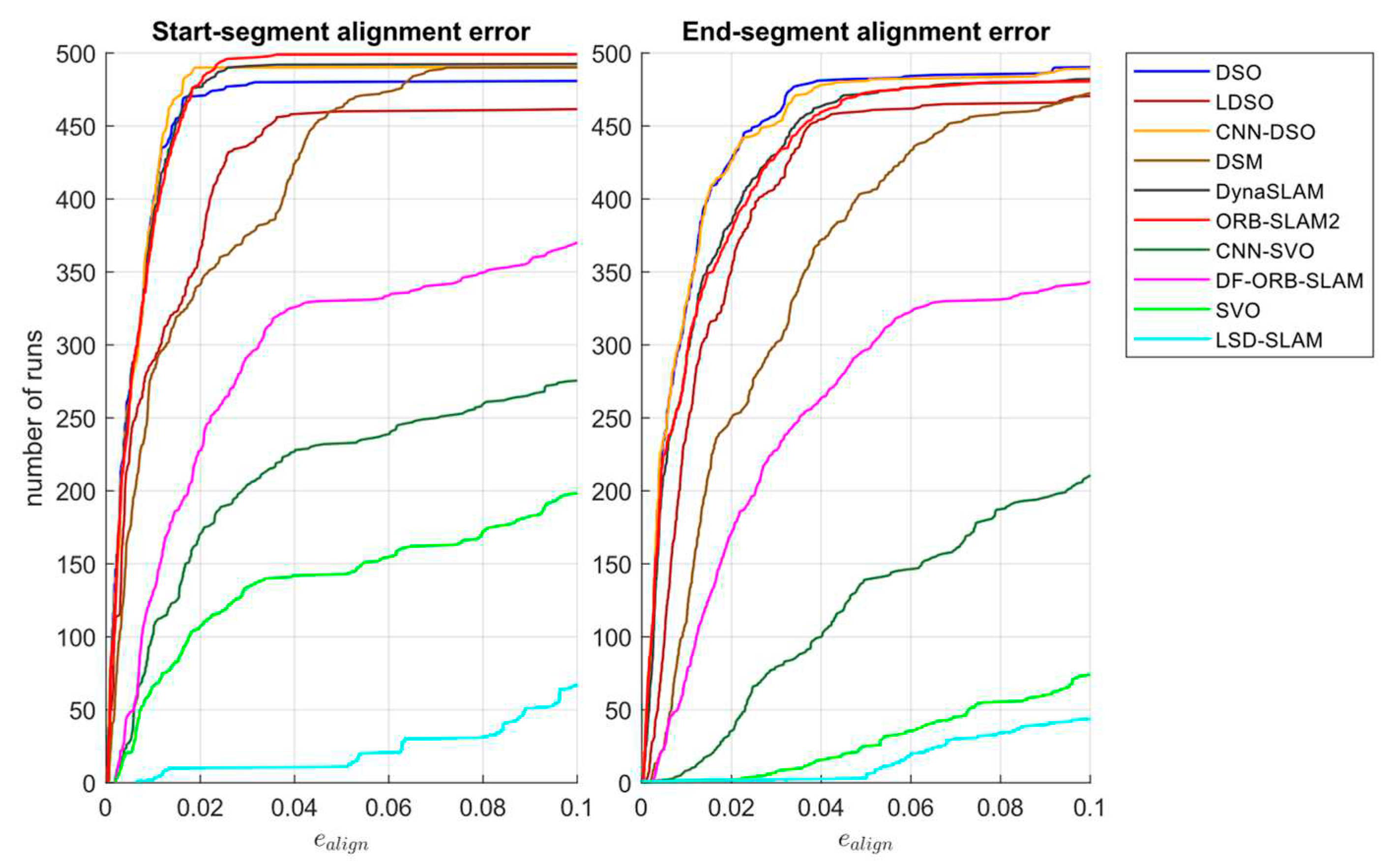
As mentioned before, the alignment error considers translation, rotation, and scale errors equally. Therefore, it is equivalent to the translational RMSE when aligned to the start and end segments (first and last 10-20 seconds of each sequence), for which the ground truth is available. The cumulated alignment error for each algorithm is presented in Figure 5.
Figure 5 shows that ORB-SLAM and DynaSLAM perform slightly better than the sparse direct methods for start-segment alignment errors. However, on the end-segment, the cumulative drift effect was lower on sparse-direct methods, which ratifies the results observed in Figure 4. In addition, it can be noticed that CNN-DSO performed better than DSO, suggesting that integrating the Single Image Depth Estimation (SIDE) CNN improved DSO bootstrapping by adding prior depth information, whereas the end-segment performance of both algorithms was similar. On the other hand, the addition of the Mask R-CNN in DynaSLAM is used to remove moving objects information from the scenes, which did not represent an improvement in the performance of the algorithm in the start-segment, but, as shown in Figure 5, the benefits of the addition of the CNN can be observed over the end-segment by the reduction of the accumulated drift. Additionally, for the hybrid approaches, the addition of the MonoDepth CNN represented an important contribution that helped to overcome the SVO loss of trajectory issues. Similarly to the results observed in Figure 1, overall alignment error results suggest that sparse-direct methods performed better, followed by sparse-indirect, dense-indirect, hybrid, and finally dense-direct, which reach the threshold error in around 50 runs.
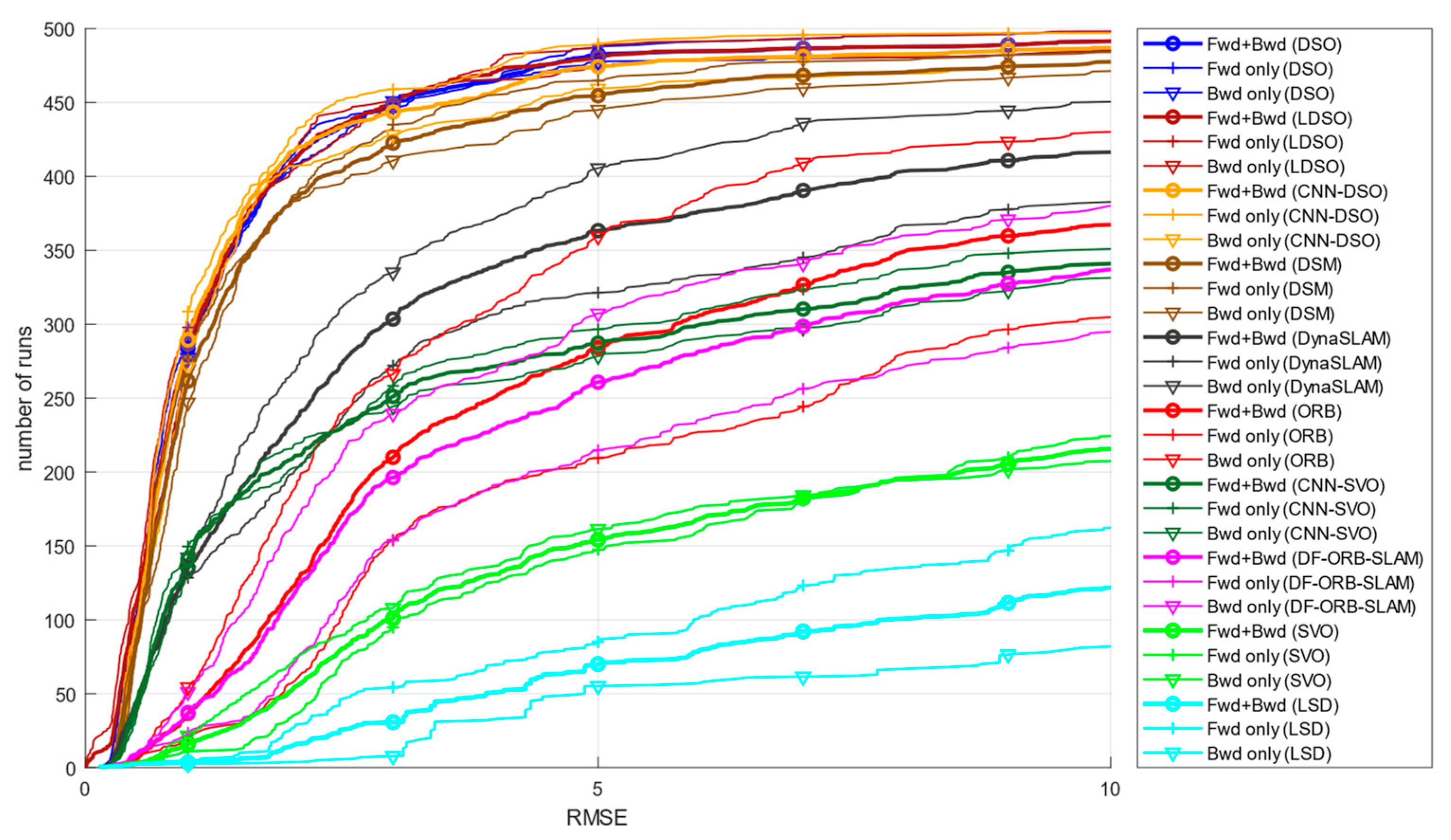
As suggested by [3], we examined dataset motion bias for each algorithm by running each method ten times forwards and ten times backward and evaluated the results in such modalities and the combination of both to visualize how much each algorithm is affected by this. This situation allowed us to consider the importance of evaluating SLAM and VO methods in large datasets, covering as much variety of environments and motion patterns as possible. The dataset motion bias for each method is presented in Figure 6.
On Figure 6, it can be noticed that DSO, LDSO, and SVO are not considerably affected by motion bias. In contrast, ORB-SLAM2, DynaSLAM, and DF-ORB-SLAM are considerably affected by different motion patterns, represented in the difference in their performance when running forwards versus backward. This behavior provides a reference of consistency and robustness of each algorithm for using them in different environments or applications. Here we also can observe that CNN-DSO on forward-only modality outperforms its classic version, but it suffers from a larger motion bias effect which affects its overall performance. In addition, DynaSLAM and CNN-SVO outperformed their classic versions and presented a smaller motion bias effect, representing an additional robustness improvement over their classic versions.
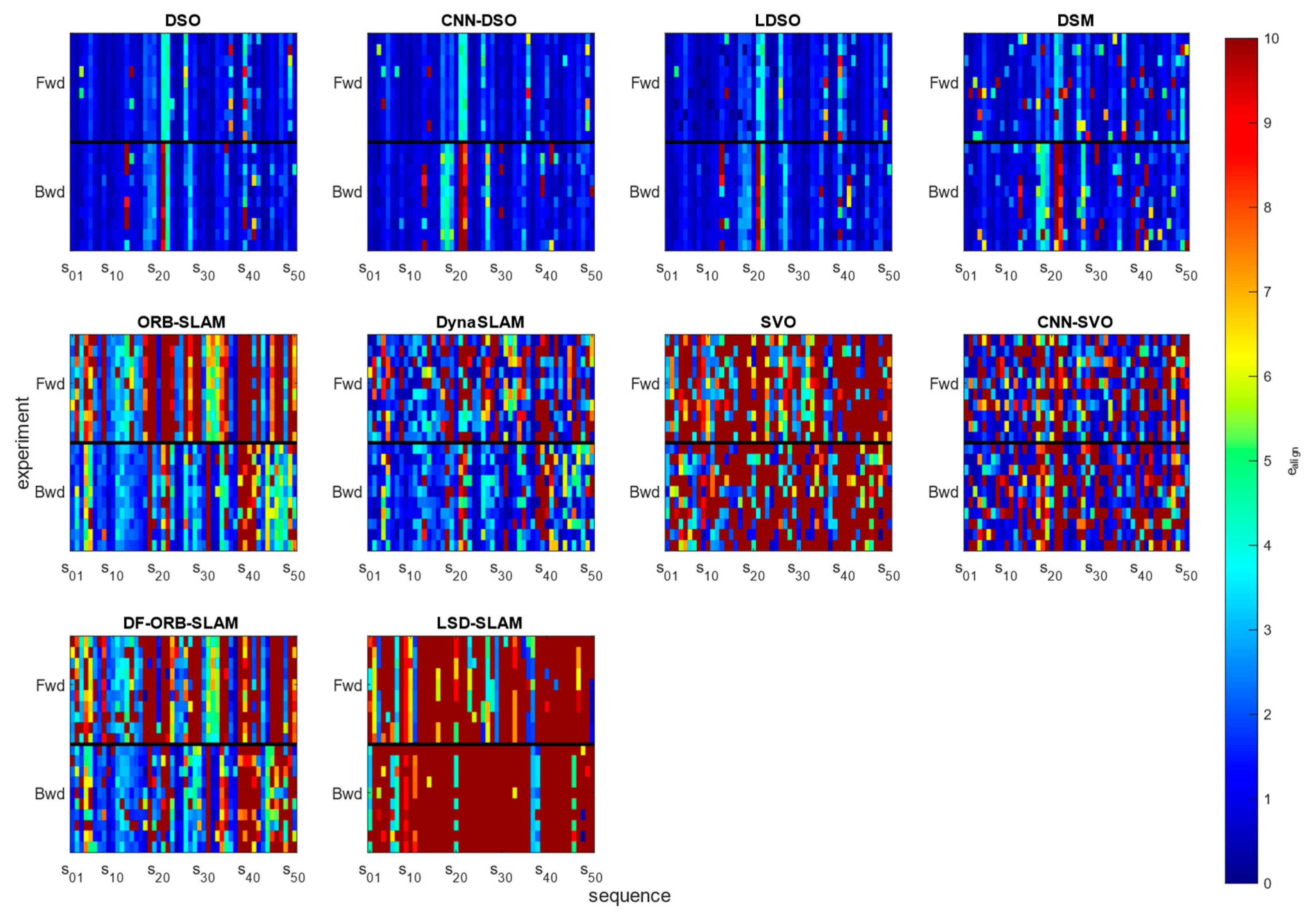
Figure 7 shows the color-coded alignment error for each of the 50 TUM-mono sequences for each run forward and backward to observe which specific sequences were challenging for each algorithm.
Figure 7, first row, presents the sparse-direct methods DSO, CNN-DSO, LDSO, and DSM, which demonstrated an outstanding performance compared to the rest of the evaluated methods that belong to the different classifications of the taxonomy, which places sparse-direct methods as the best alternative for visual odometry, SLAM, and 3D reconstruction tasks. By visualizing Figure 7, it can be noticed that CNN-DSO performs worse than the original DSO algorithm in sequences 13 and 22 but improves its performance in sequence 39. LDSO performance was close to DSO, but it presents a better trajectory in some forward sequences and overcomes DSO in sequence 21. DSM performed similarly to the rest of the sparse-direct approaches but occasionally presented trajectory loss issues that affect its overall performance. On the other hand, DynaSLAM considerably improves the performance of ORB-SLAM2, especially in challenging sequences like 18, 19, 21, 22, 23, 27, 28, 38, 39, and 40, among others, where ORB-SLAM commonly fails. However, it still occasionally presents trajectory loss and initialization issues. The optical flow implementation of ORB-SLAM2 performs slightly worse on forwards and considerably worse on backward, especially in scenes 21, 22, 38, 39, 40, 46, 48, and 50. The CNN version of SVO considerably reduced the RMSE in most sequences compared to SVO but still constantly fails in outdoor sequences 21 and 22 and presents random initialization and trajectory loss issues. As reported in [18], SVO and LSD-SLAM methods had the worst results over the whole dataset, which was why Engel et al. [18] did not include these methods in their study. However, we considered it important to report such results and errors attributed to these algorithms’ commonly known initialization and trajectory loss errors over the sequences of the TUM-mono dataset.
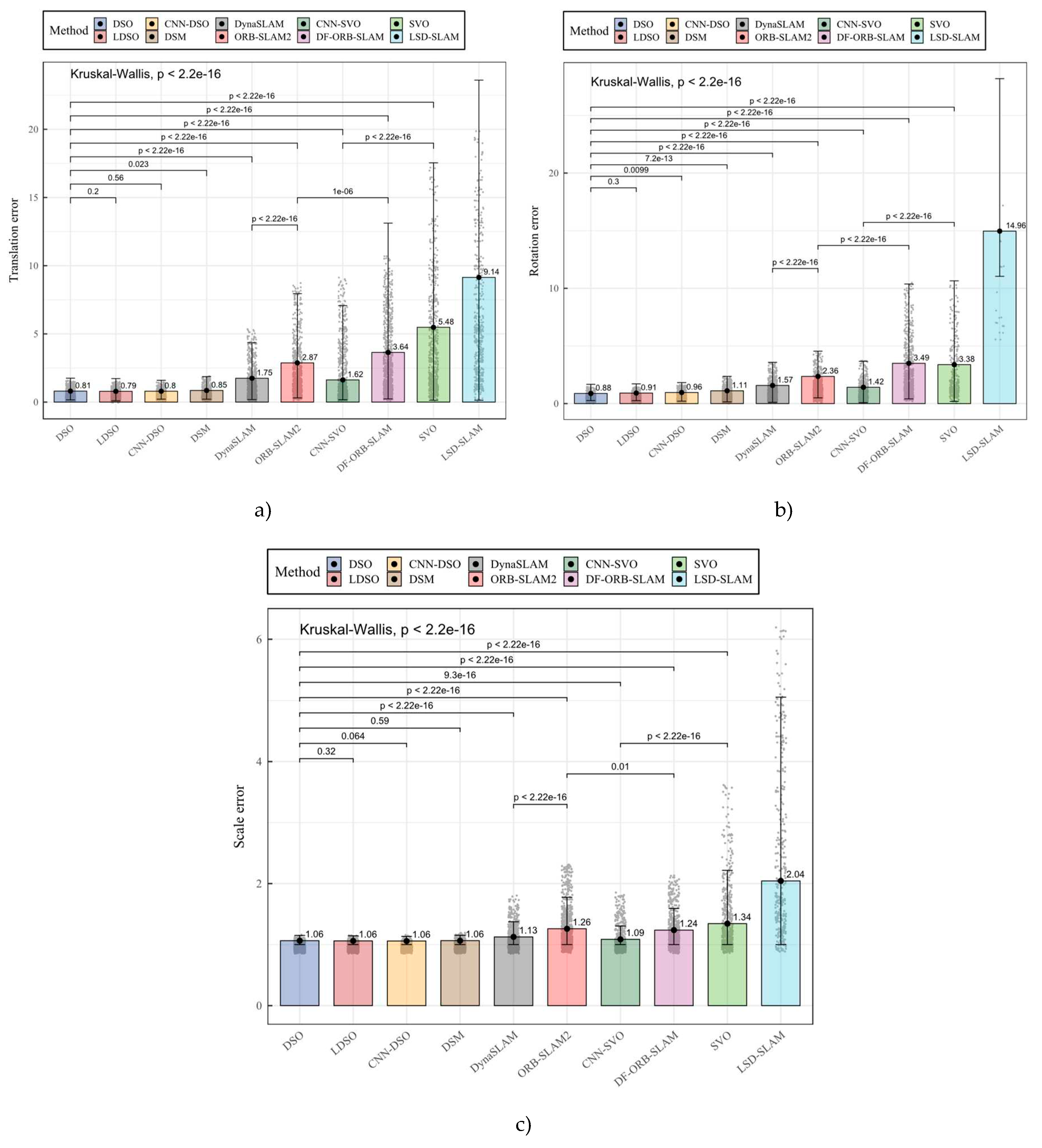
The results processed on the TUM-mono benchmark for the cumulative translation error e t , rotation error e r , scale error e s , start-segment alignment error e a l i g n s , end-segment alignment error e a l i g n e , and translational RMSE e R M S E were gathered in a database defining the method as the categoric variable. Statistic results were processed using R programing language. First, we removed blank observations for the executions where each algorithm got lost or could not initialize and applied Mahalanobis distances [73] as a multivariate data cleaning technique to detect and remove outlier observations. For this, we established a cut score of 22.4577 based on the χ 2 distribution for a 99.999% interval, so we detected 344 outlier observations ending with a database of 8860 observations.
Then, we verified the normality and homogeneity assumptions for each dependent variable to select the appropriate statistical test for comparisons. For example, for the translation error, we obtained the p-values of 2.2e-16 for all the DSO, LDSO, CNN-DSO, DSM, DynaSLAM, ORB-SLAM2, DF-ORB-SLAM, CNN-SVO, SVO and LSD-SLAM methods in the Lilliefors (Kolmogorov-Smirnov) normality test, so the sample didn’t reach the normality assumption. We applied Levene’s test obtaining a p-value of 2.2e-16 for the homogeneity assumption, so the sample did not meet the homogeneity assumption. The rest of the dependent variables had similar assumptions verification results; thus, it was concluded that the sample was not parametric, so the Kruskal-Wallis test was selected as the general test and the Wilcoxon signed rank as pairwise posthoc test. Figure 8 and Table 2 present the results obtained by applying the differences tests.
As presented in Figure 8 and Table 2, the sample allowed us to identify significant differences between the implemented algorithms. By observing the translation error, it can be noticed that DSO, LDSO, and CNN-DSO methods achieved the best significative performance of the ten evaluated algorithms, and despite DSO performing 2.18% and 1.05% worse than DSO and CNN-DSO in this metric, the difference wasn’t significative among them. DSO, LDSO, and CNN-DSO achieved significative lower errors than the dense direct method DSM. Feature-based methods performed significantly worse than sparse-direct, where DynaSLAM achieved a significative better performance than ORB-SLAM2 and DF-ORB-SLAM, reaching 39.19% and 52.02% of translation error reduction, respectively. CNN-SVO performed slightly worse than DynaSLAM, but the difference was not significant, while it significantly outperformed its classic version SVO reaching 47.57% of translation error reduction. LSD-SLAM performed significantly worse in translation error metric among the ten algorithms.
Regarding rotation error, DSO and LDSO achieved significantly better results than the rest of the algorithms. Although DSO showed an average rotation error reduction close to 3.66%, the difference was not significant. DSO performed significantly better than its neuronal version in the accumulated rotation error metric. LDSO performed around 5.02% better than CNN-DSO, but the difference was not significant. DSM performed significantly worse than the rest of the sparse-direct methods. Feature-based methods performed significantly worse than sparse-direct methods in rotation error metric, where DynaSLAM achieved a significatively better performance than ORB-SLAM2 and DF-ORB-SLAM showing an average error reduction close to 33.30% and 54.97%, respectively. CNN-SVO performed significantly better than DF-ORB-SLAM, SVO, and LSD-SLAM in rotation error metric, significantly outperforming its classic SVO version showing an average reduction of 58.07% of rotation error. LSD-SLAM performed significantly worse than the other methods in the rotation error metric.
For the scale error metric, the sparse-direct methods DSO, LDSO, and CNN-DSO performed significantly better than the rest of the methods, where CNN-DSO showed the best performance showing an average reduction of 0.49% and 0.23% compared to DSO and LDSO, but the difference was not significative. DSM performed significantly worse than CNN-DSO. Feature-based methods performed significantly worse than sparse-direct methods on the scale error metric, where DynaSLAM achieved the significatively best performance and an average reduction of 10.60% and 9.02% compared to ORB-SLAM2 and DF-ORB-SLAM. CNN-SVO performed significantly better than the feature-based methods, SVO and LSD-SLAM, exhibiting an average error reduction of 19.14% compared to its classic version, SVO. Again, LSD-SLAM got the significatively worst performance of the ten methods in the scale error metric.
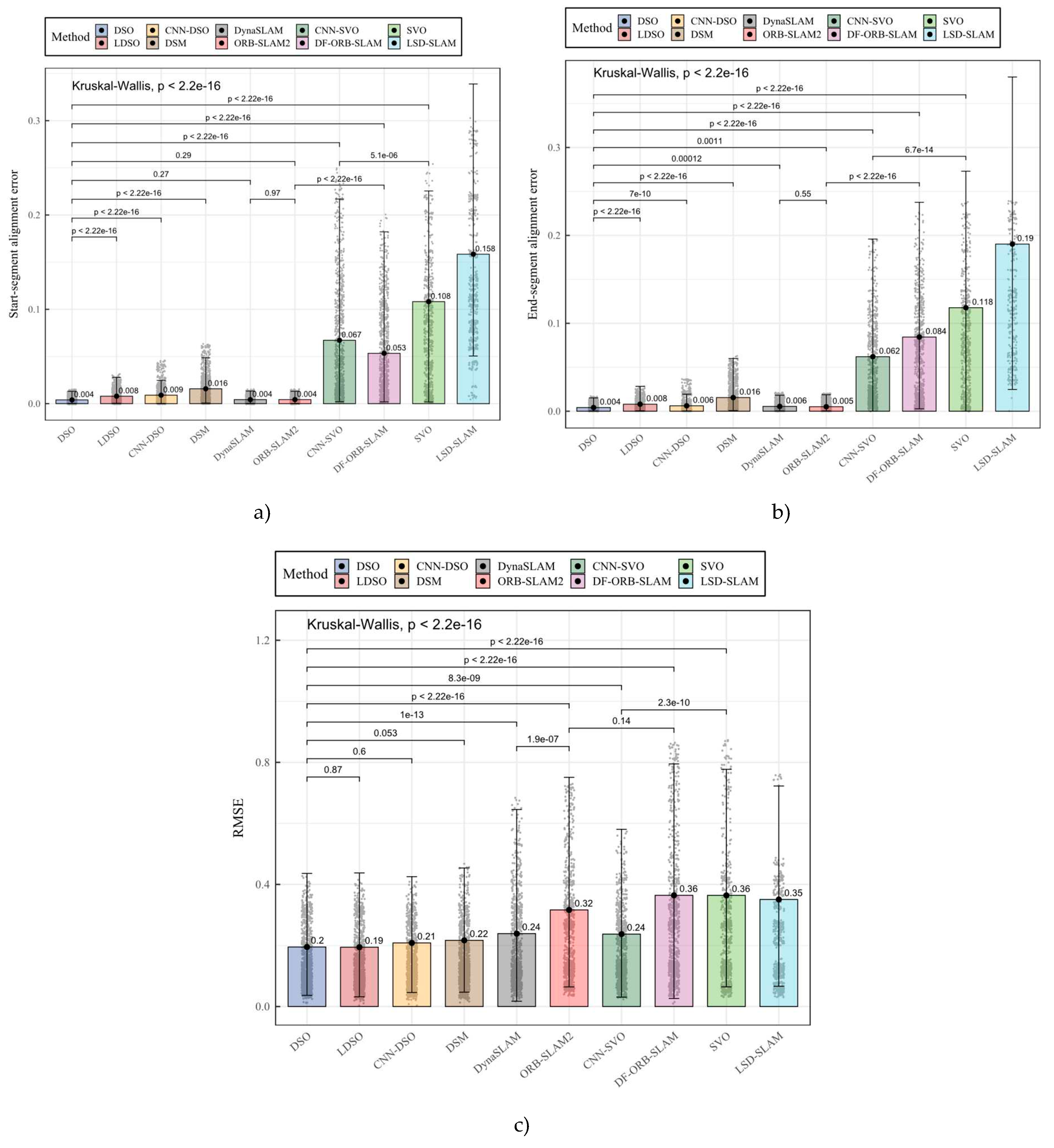
Similarly, we applied the Kruskal-Wallis test as a general test, and the Wilcoxon signed rank test for statistical comparison among the ten methods for the start- and end-segment alignment errors and the overall RMSE. Figure 9 and Table 3 present the results obtained by applying the differences tests.
Figure 9 and Table 3 show many significant differences between the ten compared methods on the alignment error and RMSE metrics. Regarding the start-segment alignment error, DSO, DynaSLAM, and ORB-SLAM methods outperform the rest of the algorithms. Despite DSO slightly reducing the average start-segment alignment error by around 7.28% and 7.81% compared to DynaSLAM and ORB-SLAM2, the differences were not significant. The rest of the sparse-direct methods, LDSO, CNN-DSO, and DSM, performed significantly worse than DSO by an average of 49.84%, 55.77%, and 74.83%, respectively, in the start-segment alignment error metric. For the feature-based methods, DynaSLAM and DSO performed significantly better than DF-ORB-SLAM, while DF-ORB-SLAM achieved an error significantly lower than CNN-SVO, SVO, and LSD-SLAM. When comparing CNN-SVO with its predecessor SVO, the difference was significant, where the neural version reduced the start-segment alignment error by an average of close to 37.86%. LSD-SLAM achieved the significantly worst start-segment alignment error of the ten methods.
By observing the end-segment alignment error, it was found that the sparse-direct methods significantly outperformed the rest of the compared methods. DSO significantly outperformed all the evaluated methods, including the rest of the sparse-direct methods, LDSO, CNN-DSO, and DSM, reducing the average alignment error to around 47.85%, 32.50%, and 73.06%, respectively. In the sparse-indirect category, DynaSLAM and ORB-SLAM2 performed significantly better than DF-ORB-SLAM, but even though ORB-SLAM2 reduced the average end-segment error by approximately 7.49%, the difference was not significative. CNN-SVO end-segment alignment error was significantly lower than the error of SVO, reducing this metric by approximately 47.31%. LDSO performed significantly worse than the rest of the methods.
For the RMSE metric, sparse-direct methods performed significantly better than the rest, where LDSO achieved RMSE values around 0.32% and 6.68% lower than DSO and CNN-DSO; the differences were not significative. LDSO performed significantly better than DSM, with an average RMSE around 10% lower. In the feature-based classification, DynaSLAM performed significantly better than ORB-SLAM2 and DF-ORB-SLAM, reducing the RMSE metric by approximately 24.49% and 34.41%, respectively. For the hybrid methods, CNN-SVO performed significantly better than SVO, reducing the RMSE by around 34.83%. Like in the rest of the metrics, LSD-SLAM performed significantly worse than the rest of the methods in the RMSE metric.
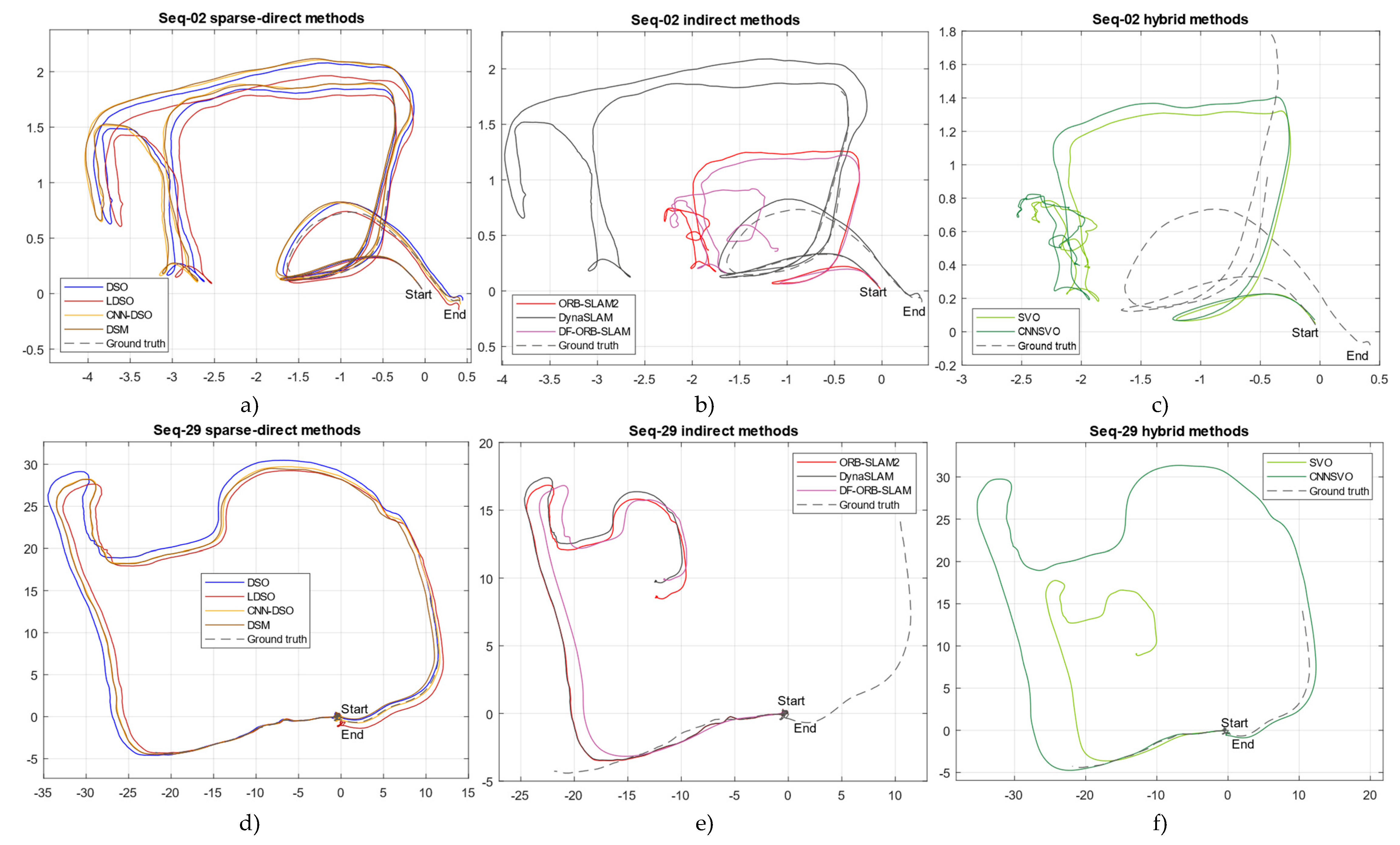
Finally, in Figure 10, we present son sample trajectories obtained by the three overall best methods evaluated in this comparison study. To exemplify the behavior of the algorithms in different environments, we selected the sequence seq-02 of the TUM-mono dataset as an example for indoors and the sequence seq-29 as an example for outdoors. In addition, we provide video samples of the execution of each algorithm as supplementary material in the GitHub repository: https://github.com/erickherreraresearch/MonocularPureVisualSLAMComparison; along with all the .txt result files of each algorithm run for reproducibility.
As depicted in Figure 10, the algorithms’ observed behavior ratifies this comparative analysis’s quantitative results. On the top row, for the indoor sequence, it can be noticed that the sparse-direct methods outperform the other evaluated methods starting and ending their trajectory pretty close to the ground truth. Indirect methods behave completely differently, where the system constantly loses the trajectory, accumulates drift, and gets wrong scale measures that are concatenated erroneously when the system achieves relocalization. It can also be noticed that DynaSLAM represent an important contribution to the ORB-SLAM2 system because it estimates the trajectory better than the rest closing the trajectory pretty close to the ground truth, while the rest of the indirect systems lost their trajectories. On the other hand, hybrid methods performed considerably worst indoors, so many of the algorithm’s runs didn’t complete the full frame sequence, and the algorithm typically finishes its trajectory pretty far from the end segment ground truth. In Figure’s 10 bottom row, it can be noticed again that sparse-direct methods outperformed the rest of the evaluated systems, with an appropriate bootstrapping in the start-segment and a small amount of accumulated drift in the end segment.
On the other hand, in Figure 10e, it can be noticed that similarly to indoors, the indirect methods suffered from trajectory loss issues and, despite the relocalization module typically achieved to continue the system execution, it accumulates a critical amount of drift during relocalization which makes the estimated trajectory end far from the ground truth end-segment. In hybrid methods, SVO suffers from similar issues to indirect methods. However, it can be noticed that the CNN version of SVO improved its performance outdoors, differently from indoors, which can be explained because the added CNN MonoDepth module was trained in the Cityscapes dataset, which was mainly trained from outdoor sequences.

4. Discussion

In the previous studies of [20,21] authors compared the DSO, LDSO, ORB-SLAM2, and DynaSLAM algorithms on the same TUM-Mono benchmark, and their findings mostly match what we observed during this evaluation. However, we extended their study considerably by implementing six additional methods following the taxonomy described in [6] and performed an appropriate statistical analysis to determine significative differences in each system’s performance. In this way, we could observe the advantages and limitations of the base classification for classic geometric-based approaches. Classic approaches can be classified as sparse-indirect, dense-indirect, dense-direct, sparse-direct, and hybrid. For sparse indirect, we selected its gold standard, ORB-SLAM2, and we can report that, in our experience, it is an excellent method that demands low computational power and has an average performance, not being the best but still working well outdoors. Its main limitations are its lousy indoor performance and large drift and scale error accumulation during relocalization. We believe that ORB-SLAM2 has reached an amazing popularity level due to its low computational power consumption and ease of implementation. For the dense-indirect category, we selected DF-ORB-SLAM, an open-source implementation of ORB-SLAM2 with an additional optical flow estimation module that allows ORB-SLAM2 to work with more image information. In this case, we observed that the optical flow module increases the computational cost of the algorithm and slightly reduces the occurrence of trajectory loss issues. However, adding image information for feature extraction also introduces noise in estimation steps, significantly increasing translation, rotation, scale error metrics, and RMSE. For dense direct approaches, we selected their gold standard, LSD-SLAM, one of the first proposed direct methods. In this case, we found that the performance was significantly the poorest of all the evaluated methods. This situation could be motivated especially because of frequent initialization errors and trajectory losses in most of the benchmark sequences, which matches what Engel et al. reported in their study [18]. For sparse-direct classification, we selected the most iconic VO system, DSO. This system significantly outperformed the methods of the rest of the classic classifications by a large margin, demonstrating an impressive performance indoors and outdoors. DSO was slightly outperformed by its neuronal version on the scale metric and slightly outperformed by LSDO in translation and RMSE metric, but the differences were not significant. This behavior lets us conclude that even its extensions LDSO, CNN-DSO, and DSM still do not significatively outperform DSO, and this method can still be considered a great avenue for future work, improvements, and contributions.
Additionally, it must be mentioned that, in contrast to what is reported in [49], the DSM method did not outperform its predecessor DSO in the TUM-mono dataset, even implementing a complete SLAM pipeline to extend DSO. We believe DSM is a robust system that can contribute to the sparse-direct category. However, the authors used the extended pinhole radial-tangential camera model instead of the complete photometrical camera calibration provided in the original DSO, which includes intrinsic, photometric, and non-parametric vignette calibration. As reported in [21], this situation contributes considerably to the correct execution of the algorithm and allows it to get the best results. Then, for the hybrid approaches, we tested SVO, which combines direct and indirect formulation paradigms in its pipeline. SVO reached second to last place in our comparison, being significantly outperformed by most of the methods of this study and only significantly performing better than LSD-SLAM, which matches what is reported in [18]. However, with this analysis, we could observe that it at least performs better than the dense-direct method. SVO is also a popular method in the robotics research field. We believe that this is caused by its early appearance in 2014, low computational power requirement, and open-source availability for implementation with C++ or ROS.
For Machine Learning (ML) classification, there exist many ML implementations available in the literature [7,11,17,51,53,54,74,75,76,77,78,79,80,81,82,83,84,85] and many of them include open source code implementations [14,16,23,24,25,26,27,28,29,30,31,32,33,80,86]. Nevertheless, many of that methods were formulated to work with more than one input modality, like RBD-D or INS, and their code implementations did not include monocular running instructions or did not include their monocular RGB pipeline, e.g., [25,33,80]. Other open-source code implementations required additional external information for their running, like optical flow or feature extractors that were not included as open source, e.g., [30]. For such reasons, we selected three ML versions of the tested classic approaches DSO, ORB-SLAM2, and SVO: CNN-DSO, DynaSLAM, and CNN-SVO. In this way, we concluded that CNN-SVO significantly outperformed its predecessor in all the metrics, DynaSLAM significantly outperformed ORB-SLAM2 in all the metrics except for the end-segment alignment error where the difference wasn’t significative, and CNN-DSO significantly outperformed its classic version only in rotation error. Here we can mention that in contrast to what is reported in the CNN-DSO official repository [12], where the algorithm was evaluated in the first eleven sequences of the KITTI dataset, after testing the algorithm in a larger dataset indoors, outdoors, and a large variety of motion patterns. We can mention that CNN-DSO only slightly outperforms DSO in the scale error metric, but the observed difference was not significant, while DSO still outperforms it in the rotation, start- and end-segment alignment error metrics. In addition, during evaluation, it was observed that the algorithm introduces a considerable amount of outlier points in the obtained 3D reconstruction. Thus, we can point out that machine learning studies are making significant contributions to improve monocular VO, SLAM, and 3D reconstruction systems. Table 4 summarizes the observed advantages and limitations of the evaluated methods based on the experience of implementing and running the algorithms.

5. Conclusions

In this article, we tested the most representative open source monocular RGB SLAM and VO available implementations, following a taxonomy to determine the advantages and limitations of each method and classification and provide the reader a guide to correctly select the method that fits their needs or, select a path to make future contributions or improvements over the tested methods and classifications. After experimentation, it can be concluded that monocular SLAM and VO methods need to be evaluated on larger datasets with a large variety of environments, motion patterns, and illumination conditions to be effectively compared with state-of-the-art, which was demonstrated in this study for methods like DSM, CNN-DSO, and DF-ORB-SLAM that did not match the expected results on TUM-Mono dataset.
The sparse-direct category of the taxonomy achieved the significatively best results of all this comparison, achieving the best performance in translation, rotation, scale, and RMSE metrics outputting the best detailed and precise 3D reconstructions of the tested methods. Second to best is placed the sparse-indirect category that achieved good ego-motion estimation but outputs sparser 3D reconstructions that might not be suitable for many applications, present trajectory loss issues, and evidenced worse performance indoors. Additionally, by including three machine learning methods and comparing them with their classic versions, we can conclude that the integration of machine learning significantly improves the performance of the SLAM or VO systems and should be considered as future research direction to overcome the limitations of each system. Integrating CNN information for the estimation steps contributes to mitigating monocular systems’ commonly known scale ambiguity issue. This behavior was demonstrated in each ML method’s significant scale error reduction compared to their classic versions.
Through experimentation [3,21] concluded that the great majority of the alignment error originated in the accumulated drift, independently from the noise in the ground truth that can be registered with any SLAM or VO system, which allows using all the metrics using the ground truth of only the start and end segments. We agree and confirm this conclusion which in our experiments allowed us to compare a wide variety of methods coming from different configurations and classifications that output trajectories in different scales and orientations, which can be efficiently compared after the proposed alignment method of the benchmark.

Funding

This work was supported by SDAS Research Group (www.sdas-group.com).

Data Availability Statement

We provide video samples of the execution of each algorithm indoors and outdoors as supplementary material in the GitHub repository: https://github.com/erickherreraresearch/MonocularPureVisualSLAMComparison along with all the .txt result files of each algorithm run for reproducibility.

Conflicts of Interest

The authors declare no conflict of interest.

References

  1. M. O. A. Aqel, M. H. Marhaban, M. I. Saripan, and N. B. Ismail, “Review of visual odometry: types, approaches, challenges, and applications,” SpringerPlus 2016 51, vol. 5, no. 1, pp. 1–26, Oct. 2016. [CrossRef]
  2. M. Zollhöfer et al., “State of the Art on Monocular 3D Face Reconstruction, Tracking, and Applications,” Comput. Graph. Forum, vol. 37, no. 2, pp. 523–550, 18. [CrossRef]
  3. J. Engel, V. Usenko, and D. Cremers, “A Photometrically Calibrated Benchmark For Monocular Visual Odometry,” Jul. 2016. [CrossRef]
  4. A. Macario Barros, M. Michel, Y. Moline, G. Corre, and F. Carrel, “A Comprehensive Survey of Visual SLAM Algorithms,” Robotics, vol. 11, no. 1, 2022. [CrossRef]
  5. A. Handa, T. Whelan, J. McDonald, and A. J. Davison, “A benchmark for RGB-D visual odometry, 3D reconstruction and SLAM,” in 2014 IEEE International Conference on Robotics and Automation (ICRA), 2014, pp. 1524–1531.
  6. E. P. Herrera-Granda, “An Extended Taxonomy for Monocular Visual SLAM, Visual Odometry, and Structure from Motion methods applied to 3D Reconstruction,” GitHub repository, 2023. [Online]. Available: https://github.com/erickherreraresearch/TaxonomyPureVisualMonocularSLAM/.
  7. K. Tateno, F. Tombari, I. Laina, and N. Navab, “CNN-SLAM: Real-time dense monocular SLAM with learned depth prediction,” in Proceedings - 30th IEEE Conference on Computer Vision and Pattern Recognition, CVPR 2017, 2017, vol. 2017-Janua, pp. 6565–6574.
  8. S. Y. Loo, A. J. Amiri, S. Mashohor, S. H. Tang, and H. Zhang, “CNN-SVO: Improving the mapping in semi-direct visual odometry using single-image depth prediction,” Proc. - IEEE Int. Conf. Robot. Autom., vol. 2019-May, pp. 5218–5223, May 2019.
  9. C. Forster, Z. Zhang, M. Gassner, M. Werlberger, and D. Scaramuzza, “SVO: Semidirect Visual Odometry for Monocular and Multicamera Systems,” IEEE Trans. Robot., vol. 33, no. 2, pp. 249–265, 2017. [CrossRef]
  10. C. Forster, M. Pizzoli, and D. Scaramuzza, “SVO: Fast semi-direct monocular visual odometry,” Proc. - IEEE Int. Conf. Robot. Autom., pp. 15–22, Sep. 2014. [CrossRef]
  11. F. Wimbauer, N. Yang, L. von Stumberg, N. Zeller, and D. Cremers, “MonoRec: Semi-Supervised Dense Reconstruction in Dynamic Environments from a Single Moving Camera,” in 2021 IEEE/CVF Conference on Computer Vision and Pattern Recognition (CVPR), 2021, pp. 6108–6118.
  12. Muskie, “CNN-DSO: A combination of Direct Sparse Odometry and CNN Depth Prediction,” GitHub repository, 2019. [Online]. Available: https://github.com/muskie82/CNN-DSO.
  13. S. Wang, “DF-ORB-SLAM,” GitHub repository, 2020. [Online]. Available: https://github.com/834810269/DF-ORB-SLAM.
  14. B. Bescos, “DynaSLAM,” GitHub repository, 2019. [Online]. Available: https://github.com/BertaBescos/DynaSLAM.
  15. J. Sun, Y. Wang, and Y. Shen, “Fully Scaled Monocular Direct Sparse Odometry with A Distance Constraint,” 2019 5th Int. Conf. Control. Autom. Robot. ICCAR 2019, pp. 271–275, Apr. 2019.
  16. A. Sundar, “CNN-SLAM,” GitHub repository, 2018. [Online]. Available: https://github.com/iitmcvg/CNN_SLAM.
  17. C. Tang and P. Tan, “BA-Net: Dense Bundle Adjustment Network,” 7th Int. Conf. Learn. Represent. ICLR 2019, Jun. 2019.
  18. J. Engel, V. Koltun, and D. Cremers, “Direct Sparse Odometry,” IEEE Trans. Pattern Anal. Mach. Intell., vol. 40, no. 3, pp. 611–625, Mar. 2017.
  19. N. Yang, R. Wang, X. Gao, and D. Cremers, “Challenges in Monocular Visual Odometry: Photometric Calibration, Motion Bias, and Rolling Shutter Effect,” IEEE Robot. Autom. Lett., vol. 3, no. 4, pp. 2878–2885, 2018.
  20. E. Mingachev, R. Lavrenov, E. Magid, and M. Svinin, “Comparative analysis of monocular slam algorithms using tum and euroc benchmarks,” in Smart Innovation, Systems and Technologies, 2021, vol. 187, pp. 343–355. [CrossRef]
  21. E. Mingachev et al., “Comparison of ROS-Based Monocular Visual SLAM Methods: DSO, LDSO, ORB-SLAM2 and DynaSLAM,” in Interactive Collaborative Robotics, 2020, pp. 222–233. [CrossRef]
  22. M. Servières, V. Renaudin, A. Dupuis, and N. Antigny, “Visual and Visual-Inertial SLAM: State of the Art, Classification, and Experimental Benchmarking,” J. Sensors, vol. 2021, p. 2054828, 2021. [CrossRef]
  23. S. Zhang, “DVSO: Deep Virtual Stereo Odometry,” GitHub repository, 2022. [Online]. Available: https://github.com/SenZHANG-GitHub/dvso.
  24. R. Cheng, “CNN-DVO,” McGill repository. McGill, 2020.
  25. F. Wimbauer and N. Yang, “MonoRec,” GitHub repository, 2017. [Online]. Available: https://github.com/Brummi/MonoRec.
  26. S. Y. Loo, “CNN-SVO,” GitHub repository, 2019. [Online]. Available: https://github.com/yan99033/CNN-SVO.
  27. A. Steenbeek, “Sparse-to-Dense: Depth Prediction from Sparse Depth Samples and a Single Image,” GitHub repository, 2022. [Online]. Available: https://github.com/annesteenbeek/sparse-to-dense-ros.
  28. B. Ummenhofer, “DeMoN: Depth and Motion Network,” GitHub repository, 2022. [Online]. Available: https://github.com/lmb-freiburg/demon.
  29. Z. Teed and J. Deng, “DeepV2D,” GitHub repository, 2020. [Online]. Available: https://github.com/princeton-vl/DeepV2D.
  30. Z. Min, “VOLDOR: Visual Odometry from Log-logistic Dense Optical flow Residual,” GitHub repository, 2020. [Online]. Available: https://github.com/htkseason/VOLDOR.
  31. Z. Teed and J. Deng, “DROID-SLAM,” GitHub repository, 2022. [Online]. Available: https://github.com/princeton-vl/DROID-SLAM.
  32. H. Zhou, B. Ummenhofer, and T. Brox, “DeepTAM,” GitHub repository, 2019. [Online]. Available: https://github.com/lmb-freiburg/deeptam.
  33. S. Troscot, “CodeSLAM,” GitHub repository, 2022. [Online]. Available: https://github.com/silviutroscot/CodeSLAM.
  34. J. Czarnowski and M. Kaneko, “DeepFactors,” GitHub repository, 2020. [Online]. Available: https://github.com/jczarnowski/DeepFactors.
  35. R. Mur-Artal and J. D. Tardos, “ORB-SLAM2: An Open-Source SLAM System for Monocular, Stereo, and RGB-D Cameras,” IEEE Trans. Robot., vol. 33, no. 5, pp. 1255–1262, Oct. 2017. [CrossRef]
  36. R. Mur-Artal, J. M. M. Montiel, and J. D. Tardos, “ORB-SLAM: A Versatile and Accurate Monocular SLAM System,” IEEE Trans. Robot., vol. 31, no. 5, pp. 1147–1163, Oct. 2015. [CrossRef]
  37. R. Mur-Artal, “ORB-SLAM2,” GitHub repository, 2017. [Online]. Available: https://github.com/raulmur/ORB_SLAM2.
  38. L. Valgaerts, A. Bruhn, M. Mainberger, and J. Weickert, “Dense versus Sparse Approaches for Estimating the Fundamental Matrix,” Int. J. Comput. Vis. 2011 962, vol. 96, no. 2, pp. 212–234, Jun. 2011. [CrossRef]
  39. R. Ranftl, V. Vineet, Q. Chen, and V. Koltun, “Dense Monocular Depth Estimation in Complex Dynamic Scenes,” Proc. IEEE Comput. Soc. Conf. Comput. Vis. Pattern Recognit., vol. 2016-Decem, pp. 4058–4066, Dec. 2016.
  40. J. Engel, T. Schöps, and D. Cremers, “LSD-SLAM: Large-Scale Direct monocular SLAM,” in Lecture Notes in Computer Science (including subseries Lecture Notes in Artificial Intelligence and Lecture Notes in Bioinformatics), 2014, vol. 8690 LNCS, no. PART 2, pp. 834–849.
  41. H. Matsuki, L. von Stumberg, V. Usenko, J. Stückler, and D. Cremers, “Omnidirectional DSO: Direct Sparse Odometry With Fisheye Cameras,” IEEE Robot. Autom. Lett., vol. 3, no. 4, pp. 3693–3700, 2018. [CrossRef]
  42. J. Engel, J. Sturm, and D. Cremers, “Semi-dense visual odometry for a monocular camera,” in Proceedings of the IEEE International Conference on Computer Vision, 2013, pp. 1449–1456.
  43. M. Cummins and P. Newman, “FAB-MAP: Probabilistic Localization and Mapping in the Space of Appearance:,” http://dx.doi.org/10.1177/0278364908090961, vol. 27, no. 6, pp. 647–665, Jun. 2008.
  44. J. Engel, “LSD-SLAM: Large-Scale Direct Monocular SLAM,” GitHub repository, 2014. [Online]. Available: https://github.com/tum-vision/lsd_slam.
  45. J. Engel, “DSO: Direct Sparse Odometry,” GitHub repository, 2017. [Online]. Available: https://github.com/JakobEngel/dso.
  46. C. Forster, “Semi-direct monocular visual odometry,” GitHub repository, 2017. [Online]. Available: https://github.com/uzh-rpg/rpg_svo.
  47. X. Gao, R. Wang, N. Demmel, and D. Cremers, “LDSO: Direct Sparse Odometry with Loop Closure,” IEEE Int. Conf. Intell. Robot. Syst., pp. 2198–2204, Dec. 2018. [CrossRef]
  48. N. Demmel, G. Xiang, and U. Erkam, “LDSO: Direct Sparse Odometry with Loop Closure,” GitHub repository, 2020. [Online]. Available: https://github.com/tum-vision/LDSO.
  49. J. Zubizarreta, I. Aguinaga, and J. M. M. Montiel, “Direct Sparse Mapping,” IEEE Trans. Robot., vol. 36, no. 4, pp. 1363–1370, 2020. [CrossRef]
  50. J. Zubizarreta, “DSM: Direct Sparse Mapping,” GitHub repository, 2021. [Online]. Available: https://github.com/jzubizarreta/dsm.
  51. B. Bescos, J. M. Fácil, J. Civera, and J. Neira, “DynaSLAM: Tracking, Mapping, and Inpainting in Dynamic Scenes,” IEEE Robot. Autom. Lett., vol. 3, no. 4, pp. 4076–4083, 2018. [CrossRef]
  52. K. He, G. Gkioxari, P. Dollár, and R. Girshick, “Mask R-CNN,” in 2017 IEEE International Conference on Computer Vision (ICCV), 2017, pp. 2980–2988.
  53. N. Yang, L. von Stumberg, R. Wang, and D. Cremers, “D3VO: Deep Depth, Deep Pose and Deep Uncertainty for Monocular Visual Odometry,” in 2020 IEEE/CVF Conference on Computer Vision and Pattern Recognition (CVPR), 2020, pp. 1278–1289.
  54. C. Zhao, Y. Tang, Q. Sun, and A. V. Vasilakos, “Deep Direct Visual Odometry,” IEEE Trans. Intell. Transp. Syst., 2021.
  55. C. Godard, O. Mac Aodha, and G. J. Brostow, “Unsupervised Monocular Depth Estimation with Left-Right Consistency.” 2017.
  56. S. Y. Loo, “MonoDepth CPP,” 2021. [Online]. Available: https://github.com/yan99033/monodepth-cpp.
  57. M. Cordts et al., “The Cityscapes Dataset for Semantic Urban Scene Understanding,” in 2016 IEEE Conference on Computer Vision and Pattern Recognition (CVPR), 2016, pp. 3213–3223.
  58. X. Huang et al., “The ApolloScape Dataset for Autonomous Driving,” in 2018 IEEE/CVF Conference on Computer Vision and Pattern Recognition Workshops (CVPRW), 2018, pp. 1067–10676.
  59. A. Geiger, P. Lenz, and R. Urtasun, “Are we ready for autonomous driving? The KITTI vision benchmark suite,” in 2012 IEEE Conference on Computer Vision and Pattern Recognition, 2012, pp. 3354–3361.
  60. M. Burri et al., “The EuRoC micro aerial vehicle datasets:,” https://doi.org/10.1177/0278364915620033, vol. 35, no. 10, pp. 1157–1163, Jan. 2016.
  61. D. J. Butler, J. Wulff, G. B. Stanley, and M. J. Black, “A naturalistic open source movie for optical flow evaluation,” in European Conf. on Computer Vision (ECCV), 2012, pp. 611–625.
  62. A. R. Zamir, A. Sax, W. Shen, L. Guibas, J. Malik, and S. Savarese, “Taskonomy: Disentangling Task Transfer Learning,” in 2018 IEEE/CVF Conference on Computer Vision and Pattern Recognition, 2018, pp. 3712–3722.
  63. W. Yin, Y. Liu, and C. Shen, “Virtual Normal: Enforcing Geometric Constraints for Accurate and Robust Depth Prediction,” IEEE Trans. Pattern Anal. Mach. Intell., p. 1, 2021.
  64. J. Cho, D. Min, Y. Kim, and K. Sohn, “A Large RGB-D Dataset for Semi-supervised Monocular Depth Estimation.” arXiv, 2019. [CrossRef]
  65. K. Xian et al., “Monocular Relative Depth Perception with Web Stereo Data Supervision,” in 2018 IEEE/CVF Conference on Computer Vision and Pattern Recognition, 2018, pp. 311–320.
  66. J. Sturm, N. Engelhard, F. Endres, W. Burgard, and D. Cremers, “A benchmark for the evaluation of RGB-D SLAM systems,” in 2012 IEEE/RSJ International Conference on Intelligent Robots and Systems, 2012, pp. 573–580.
  67. B. K. P. Horn, “Closed-form solution of absolute orientation using unit quaternions,” J. Opt. Soc. Am. A, vol. 4, no. 4, pp. 629–642, Apr. 1987. [CrossRef]
  68. S. Sarabandi and F. Thomas, “Accurate Computation of Quaternions from Rotation Matrices,” in Advances in Robot Kinematics 2018, 2019, pp. 39–46.
  69. F. Devernay and O. Faugeras, “Straight lines have to be straight,” Mach. Vis. Appl., vol. 13, no. 1, pp. 14–24, 2001. [CrossRef]
  70. R. Castle, “PTAM-GPL: Parallel Tracking and Mapping,” GitHub repository, 2013. [Online]. Available: https://github.com/Oxford-PTAM/PTAM-GPL.
  71. ROS.org, “ROS Camera Calibration,” 2020. [Online]. Available: http://wiki.ros.org/camera_calibration. [Accessed: 26-Dec-2022].
  72. Open Source Computer Vision.org, “Camera calibration with OpenCV,” 2019. [Online]. Available: https://docs.opencv.org/4.1.1/d4/d94/tutorial_camera_calibration.html. [Accessed: 26-Dec-2022].
  73. H. Ghorbani, “MAHALANOBIS DISTANCE AND ITS APPLICATION FOR DETECTING MULTIVARIATE OUTLIERS,” FACTA Univ. Ser. Math. INFORMATICS, vol. 34, pp. 583–595, 2019.
  74. Z. Min and E. Dunn, “VOLDOR-SLAM: For the Times When Feature-Based or Direct Methods Are Not Good Enough,” CoRR, vol. abs/2104.0, 2021.
  75. Z. Teed and J. Deng, “DROID-SLAM: Deep Visual SLAM for Monocular, Stereo, and RGB-D Cameras.” arXiv, 2021.
  76. C. Yang, Q. Chen, Y. Yang, J. Zhang, M. Wu, and K. Mei, “SDF-SLAM: A Deep Learning Based Highly Accurate SLAM Using Monocular Camera Aiming at Indoor Map Reconstruction With Semantic and Depth Fusion,” IEEE Access, vol. 10, pp. 10259–10272, 2022. [CrossRef]
  77. H. Zhou, B. Ummenhofer, and T. Brox, “DeepTAM: Deep Tracking and Mapping with Convolutional Neural Networks,” Int. J. Comput. Vis., vol. 128, no. 3, pp. 756–769, Mar. 2020. [CrossRef]
  78. T. Laidlow, J. Czarnowski, and S. Leutenegger, “DeepFusion: Real-time dense 3D reconstruction for monocular SLAM using single-view depth and gradient predictions,” in Proceedings - IEEE International Conference on Robotics and Automation, 2019, vol. 2019-May, pp. 4068–4074.
  79. M. Bloesch, J. Czarnowski, R. Clark, S. Leutenegger, and A. J. Davison, “CodeSLAM - Learning a Compact, Optimisable Representation for Dense Visual SLAM,” in Proceedings of the IEEE Computer Society Conference on Computer Vision and Pattern Recognition, 2018, pp. 2560–2568.
  80. J. Czarnowski, T. Laidlow, R. Clark, and A. J. Davison, “DeepFactors: Real-Time Probabilistic Dense Monocular SLAM,” IEEE Robot. Autom. Lett., vol. 5, no. 2, pp. 721–728, Apr. 2020. [CrossRef]
  81. N. Yang, R. Wang, J. Stückler, and D. Cremers, “Deep Virtual Stereo Odometry: Leveraging Deep Depth Prediction for Monocular Direct Sparse Odometry.” arXiv, 2018.
  82. A. Steenbeek and F. Nex, “CNN-Based Dense Monocular Visual SLAM for Real-Time UAV Exploration in Emergency Conditions,” Drones, vol. 6, no. 3, 2022. [CrossRef]
  83. L. Sun, W. Yin, E. Xie, Z. Li, C. Sun, and C. Shen, “Improving Monocular Visual Odometry Using Learned Depth,” IEEE Trans. Robot., pp. 1–14, 2022. [CrossRef]
  84. B. Ummenhofer et al., “DeMoN: Depth and motion network for learning monocular stereo,” Proc. - 30th IEEE Conf. Comput. Vis. Pattern Recognition, CVPR 2017, vol. 2017-January, pp. 5622–5631, Nov. 2017.
  85. Z. Teed and J. Deng, “DeepV2D: Video to Depth with Differentiable Structure from Motion.” arXiv, 2020.
  86. C. Tang, “BA-Net: Dense Bundle Adjustment Network,” GitHub repository, 2020. [Online]. Available: https://github.com/frobelbest/BANet.
Figure 1. Diagram of the SLAM, SFM, and VO taxonomy. Inspired by the work [6].
Preprints 78725 g001
Figure 2. Examples of executions of each algorithm for the indoor sequence seq-01 of the TUM-Mono dataset. The implemented methods were: a) ORB-SLAM2, b) DF-ORB-SLAM, c) LSD-SLAM, d) DSO, e) CNN-DSO, f) LDSO, g) DSM, h) DynaSLAM, i) SVO and j) CNN-SVO.
Preprints 78725 g002
Figure 3. Examples of executions of each algorithm for the outdoor sequence seq-02 of the TUM-Mono dataset. The implemented methods were: a) ORB-SLAM2, b) DF-ORB-SLAM, c) LSD-SLAM, d) DSO, e) CNN-DSO, f) LDSO, g) DSM, h) DynaSLAM, i) SVO and j) CNN-SVO.
Preprints 78725 g003aPreprints 78725 g003b
Figure 4. Translation e t , rotation e r , and scale e s accumulated errors for the ten evaluated algorithms.
Preprints 78725 g004
Figure 5. Start- and end-segment alignment error, corresponding to the RMSE of the alignment error when compared with the start- and end-segment ground truth.
Preprints 78725 g005
Figure 6. Dataset motion bias for each method was evaluated by running all sequences forwards and backward, as well as their combination (bold).
Preprints 78725 g006
Figure 7. Color-coded alignment error e a l i g n for each algorithm in the TUM-mono dataset.
Preprints 78725 g007
Figure 8. Bar-plots, box-plot error bars, and Kruskal-Wallis comparisons for the medians of the cumulative errors collected after 1000 runs of each algorithm, a) translation error, b) rotation error, and c) scale error.
Preprints 78725 g008
Figure 9. Bar-plots, box-plot error bars, and Kruskal-Wallis comparisons for the medians of the cumulative errors collected after 1000 runs of each algorithm, a) only start-segment alignment error, b) only end-segment alignment error, c) RMSE for combined effect on start and end segments.
Preprints 78725 g009
Figure 10. Trajectories in TUM-Mono dataset for the compared sparse-direct a) d), indirect b) e) and hybrid methods c) f). The top row displays the results for the indoor sequence seq-02, and the bottom row displays the results for the outdoor sequence seq-29. Solid lines represent the trajectory estimated by each algorithm, and dashed lines represent the aligned ground truth.
Preprints 78725 g010
Table 1. Specifications of the hardware used during experimentation.
Component Specifications
CPU AMD Ryzen™ 7 3800X, eight cores, 16 threads, 3.9 – 4.5 GHz.
GPU NVIDIA GEFORCE GTX 1080 Ti. Pascal architecture, 1582 MHz, 3584 CUDA cores, 11 GB GDDR5X.
RAM 16 GB, DDR 4, 3200 MHz
ROM SSD NVME M.2 Western Digital 7300 MB/s
Power consumption 750 W1
1 Hardware did not reach max power consumption. Avg. load was close to 600 W during experiments.
Table 2. Medians and Kruskal-Wallis comparisons for each algorithm’s translation, rotation, and scale errors.
Method Translation error Rotation error Scale error
Kruskal-Wallis general test χ 2 = 3582.9   p v a l u e = 2.2 e 16 χ 2 = 2278.4   p v a l u e = 2.2 e 16 χ 2 = 2419.1   p v a l u e = 2.2 e 16
DSO 0.8064585a 0.8800369b 1.064086ab
LDSO 0.7892125a 0.9135608ab 1.061302ab
CNN-DSO 0.7980411a 0.9618528a 1.058849a
DSM 0.8519143b 1.1117710c 1.064615b
DynaSLAM 1.7473504c 1.5730542d 1.126499c
ORB-SLAM2 2.8738313d 2.3585843e 1.260155d
CNN-SVO 1.6248001c 1.4159545d 1.086399e
DF-ORB-SLAM 3.6423921e 3.4940400f 1.238232f
SVO 5.4819407f 3.3772024f 1.343603g
LSD-SLAM 9.1403348g 14.9621188g 2.044298h
Means with different letters in the same column differ significantly according to the Kruskal-Wallis test and pairwise Wilcoxon signed rank test for p v a l u e 0.05 .
Table 3. Medians and Kruskal-Wallis comparisons for translation errors of each algorithm.
Method Start-segment
alignment error
End-segment
alignment error
RMSE
Kruskal-Wallis general test χ 2 = 4575.7   p v a l u e = 2.2 e 16 χ 2 = 3718   p v a l u e = 2.2 e 16 χ 2 = 530.78   p v a l u e = 2.2 e 16
DSO 0.003974759a 0.004184367a 0.1950799ab
LDSO 0.007925665b 0.008009198b 0.1944492a
CNN-DSO 0.008987173b 0.006199582c 0.2083872ab
DSM 0.015794222c 0.015537213d 0.2167750b
DynaSLAM 0.004286919a 0.005516179e 0.2389837cd
ORB-SLAM2 0.004311949a 0.005102672e 0.3165024e
CNN-SVO 0.067201999d 0.062036008f 0.2373532c
DF-ORB-SLAM 0.053360456e 0.084420570g 0.3643844e
SVO 0.108150349f 0.117753996h 0.3642558e
LSD-SLAM 0.158469383g 0.190127787i 0.3507099d
Means with different letters in the same column differ significantly according to the Kruskal-Wallis test and pairwise Wilcoxon signed rank test for p v a l u e 0.05 .
Table 4. Practical advantages and limitations of the evaluated methods.
Method. Category Advantages Limitations
ORB-SLAM2 [35] Classic-sparse-indirect Low computational cost. Multiple input modalities. Easy to implement. Robustness to multiple environments. Trajectory loss issues. Accumulates drift while relocalizing. Sparse 3D reconstruction.
DF-ORB-SLAM [13] Classic-dense- indirect Low computational cost. Reduces trajectory loss issues. Introduces noise for trajectory estimation. Accumulates drift on relocalization. Sparse 3D reconstruction. Reduces the performance of ORB-SLAM2 significantly.
LSD-SLAM [40] Classic-dense-direct Low computational cost. More detailed 3D reconstruction, but with the presence of outliers. Includes more information in the final 3D reconstruction. Poorest performance of the evaluated methods. Initialization issues. Trajectory loss issues.
DSO [18] Classic-sparse-direct Low computational cost. Easy to implement. More detailed and precise 3D reconstruction. Robust to multiple environments and motion patterns. Best performance of all methods in most of the metrics. Requires specific complex camera calibration. Slightly but outperformed by LDSO in translation and RMSE metrics, but the differences were not significant.
SVO [10] Classic-hybrid Low computational cost. Good documentation and open-source availability for implementation in diverse configurations. Frequent trajectory loss issues. Initialization issues. Critical execution errors due to the absence of a relocalization module.
LDSO [47] Classic-sparse-direct Low computational cost. Similar to DSO, detailed and precise 3D reconstruction. Easy to implement. Includes loop closure module. Slightly outperforms DSO in translation and rotation error, but the differences were not significant. Best performance in translation and RMSE metrics than DSO, but the differences weren’t significant. Requires specific complex camera calibration. Performs significantly worse than DSO in the end-segment error metric.
DSM [49] Classic-sparse-direct Detailed and precise 3D reconstruction. Robust execution in most of the environments and motion patterns. Complete and interactive GUI. Requires more computational capabilities than the rest of sparse-direct methods. Significatively underperformed most of the sparse-direct methods.
CNN-DSO [12] ML-sparse-direct Detailed and precise 3D reconstruction. Robust to multiple environments and motion patterns. Significant best performance in scale error metric. Presence of outliers in the 3D reconstruction. Significatively outperformed in rotation error metric by DSO. Difficult to implement. Specific hardware is required.
DynaSLAM [51] ML-sparse-indirect Multiple input modalities. Easy to implement. Robustness to multiple environments. Detects, segments, and removes information of moving objects. Especially recommended for dynamic environments. Less trajectory loss issues than ORB-SLAM2. Accumulates drift while relocalizing. Sparse 3D reconstruction. Increases complexity to ORB-SLAM2. Specific hardware is required.
CNN-SVO [8] ML-hybrid Considerably reduces trajectory loss issues of SVO. Initialization issues. Reduces the number of execution issues compared to SVO. Outperforms ORB-SLAM2 in the rotation, translation, scale, and RMSE metrics. Significantly outperforms its classic version in all the metrics. Considerable presence of outliers in the 3D reconstruction. Imprecise and sparser 3D reconstruction. Complex implementation. Specific hardware is required.
Disclaimer/Publisher’s Note: The statements, opinions and data contained in all publications are solely those of the individual author(s) and contributor(s) and not of MDPI and/or the editor(s). MDPI and/or the editor(s) disclaim responsibility for any injury to people or property resulting from any ideas, methods, instructions or products referred to in the content.
Copyright: This open access article is published under a Creative Commons CC BY 4.0 license, which permit the free download, distribution, and reuse, provided that the author and preprint are cited in any reuse.
Prerpints.org logo

Preprints.org is a free preprint server supported by MDPI in Basel, Switzerland.

Subscribe

© 2024 MDPI (Basel, Switzerland) unless otherwise stated