1. Introduction
Advancements in quantum computing (QC) are paving the way for a new age in simulations, promising to revolutionize several industry verticals, including communications, finance, medicine, materials, artificial intelligence, cryptography, etc., over the coming decades. The enormous potential for QC to tackle extremely complex issues is garnering ever greater interest as the capabilities of conventional computer systems are rapidly approaching their limits, and efforts globally to mount up the quantum race are intensifying. This disruptive and rapidly emerging new technology represents both a radical change in the laws of physics in computing as we know them and a huge, unimaginable opportunity, which is expected to result in significant changes to many aspects of modern life. Since its first conceptualization in the 1980s and early proof of principles for hardware in the 2000s, quantum computers can now be built with hundreds of qubits thanks to the progress made by companies, start-ups and corporations.
In contrast to classical computing, QC harnesses the laws of quantum mechanics to solve problems that are considered intractable for classical computers by exploiting counter-intuitive quantum physical phenomena like superposition and entanglement. Despite the fundamental differences between classical and quantum computing, any computational problem solvable by a classical computer can also be solved by a quantum computer, and vice versa, as stated by the Church-Turing thesis. However, certain quantum algorithms are demonstrated to have significantly lower time and/or memory complexity than corresponding known classical algorithms and are even expected to solve problems that no classical computer could in any feasible amount of time, a feat known as “quantum supremacy”. Examples include the famous Schor factoring algorithm [
1] and the Grover search algorithm [
2]. Therefore, the potential of quantum computing for scientific and industrial breakthroughs is immense, which justifies the considerable research devoted to its application in real-world problems.
Even though quantum technology is still in its infancy, the rapid development of quantum hardware and the enormous monetary investments made worldwide have led many to claim that the so-called Noisy-Intermediate Scale Quantum (NISQ) devices already in existence may soon outperform conventional computers. In short, NISQ devices are near-term quantum computers with insufficient physical qubits to execute effective error-correcting techniques. On a handful of problems created specifically for assessing the capabilities of quantum computers, it already has been demonstrated that existing NISQ computers outperform classical computers. The algorithms that run on these constrained devices may only need a few qubits, exhibit some noise resilience, and are frequently implemented as hybrid algorithms, where some operations are carried out on a quantum device and some on a classical computer. Particularly, the number of operations, or quantum gates, must be kept to a minimum since the more errors that are introduced into the quantum state during implementation, the greater the likelihood that the quantum state may decohere. Due to these restrictions, there are limits on the scope of algorithms that can be considered. Therefore, the crucial technological question is how to best utilize current NISQ technology to get a quantum advantage. Any such strategy must account for a limited number of qubits, limited connectivity of the qubits, and coherent and incoherent errors that limit quantum circuit depth.
In parallel, the field of computational science and engineering (CSE) is also exponentially growing, being inextricably linked to the quest of solving problems of rising complexity. In this environment, quantum computing is expected to bring tremendous breakthroughs to this field. Even to this day, many critical problems lay beyond our current computational capabilities and are deemed intractable even for the world’s most advanced supercomputers. Some examples are non-convex optimization problems, modeling physical systems at multiple length and/or time scales, molecular modeling, robust design problems, and others. With quantum computing coming to the fore, there is a silver lining in the computing world that one can finally solve such complex problems. Towards this direction, quantum variants of classical algorithms have been recently proposed for solving linear systems of algebraic equations [
3] and differential equations [
4], as well as for performing optimization [
5,
6] and machine learning [
7,
8,
9] in quantum computers. All these problems lie at the heart of CSE and incorporating new quantum technologies may lead to unforeseeable advances in the field. Nevertheless, we are still in the NISQ era and there are still several obstacles and limitations that hinder the application of quantum algorithms in the field of CSE. Current state-of-the-art quantum technologies solve at best a very limited set of problems and it’s unlikely that there will be available general-purpose quantum computers in the near future that can solve problems more quickly than classical computers do. In addition, even quantum algorithms that are known to be faster than their classical counterparts most often require a fair amount of preparation done on a classical computer, either to set up the problem and/or interpret the answer.
Based on these, it becomes evident that quantum computing utilization requires efficient synergy with classical computing. In this regard, variational quantum algorithms (VQAs) have emerged as the leading strategy to obtain a quantum advantage on NISQ devices. VQAs are hybrid quantum-classical algorithms that consist of a parameterized quantum circuit, that is an ansatz of gates containing tunable parameters, and an optimization part performed on a classical computer to find the optimal values of the parameters in the circuit. Most prominent examples in this category include the VQLS algorithm [
10,
11] for solving linear systems of equations, the Quantum Approximate Optimization algorithm (QAOA) [
5] and the Quantum Analytic Descent algorithm (QAD) [
12] for optimization problems, as well as the Variational Quantum Eigensolver (VQE) [
13], tasked with finding the lowest eigenvalue of a given matrix.
This work proposes a methodology that fuses hybrid quantum algorithms and in particular the VQLS algorithm, with machine learning to accelerate the solution of parameterized linear systems. Such systems arise frequently in CSE applications in the context of uncertainty propagation, parameter inference, optimization, or sensitivity analysis, since these problems are governed by parameterized partial differential equations that are converted to linear systems using numerical discretization methods (typically, finite element or finite difference methods). A general approach to treat these types of problems is to evaluate the system response for multiple parameter instances and post-process the results to extract relevant information on quantities of interest. However, this can be a computationally intensive process, especially when the linear systems under consideration are of high dimensionality. In this regard, this work explores the use of the VQLS algorithm as the main tool to solve parametrized linear systems and investigates ways to accelerate its convergence for a given snapshot of parameters by employing machine learning algorithms to efficiently deliver accurate predictions on the optimal circuit parameters of the corresponding linear system. The main intuition behind this approach is that successful initial prediction on the circuit parameters will reduce the number of iterations of the classical optimizer employed by the VQLS algorithm.
The paper is structured as follows: In
Section 2 the fundamental principles of quantum computing are presented.
Section 3 provides the mathematical and algorithmic background for the VQLS algorithm.
Section 4 presents a methodology that utilizes machine learning to accelerate the convergence of the VQLS algorithm when used for solving parameterized linear systems.
Section 5 demonstrates the proposed methodology in a set of numerical applications and, lastly,
Section 5 summarizes the conclusions drawn from this work and discusses future research directions.
2. Basic Principles of Quantum Computing
Initially, we shall introduce the basic principles of quantum computing and specifically the well-established
Circuit /or
Gate paradigm, on which VQLS is based. Most famous algorithms, s.a. Shor’s for prime factoring [
1] or HHL for linear systems [
3], follow this paradigm.
2.1. Quantum Computation
A quantum computation is composed of three steps: input state preparation, transformations acting on this state and, finally, measurement of the output state. Due to the stochastic nature of quantum objects, the only way to gain part of the information hidden in a quantum state is by sampling, i.e. repeating the quantum algorithm several times and extracting probabilistic measures.
The elementary memory unit of QC is the
qubit, a 2-level quantum system that can be prepared, manipulated and measured in a predefined way. Unlike a classical bit, which can take the distinct value of either 0 or 1, a qubit can be a linear combination — or superposition— of two orthogonal quantum states |0〉 and |1〉. Thus, using Dirac notation, a single-qubit system can be described as
where the coefficients
are called
amplitudes of the state adhering to the constraint
.
Since not much can be achieved with a single-qubit system, multi-qubit systems can be produced by taking advantage of the peculiar quantum-mechanical properties of superposition and entanglement. Hence, an
n-qubit state, which resides in a
-dimensional complex Hilbert space, can be written as
where
the amplitudes following the normalization constraint
. The probability of measuring a particular outcome,
, is given by the squared magnitude of the corresponding amplitude,
. As mentioned, in order to calculate that probability, one has to repeatedly take measurements of output state.
Quantum computers use quantum gates, which are elementary operations that manipulate the quantum state of a system, to perform calculations. some of the most notable single-qubit gates are the Pauli gates and the Hadamard gate H. These gates are represented by unitary matrices, denoted as U and preserve the inner product between quantum states.
An example of a single-qubit circuit is illustrated in
Figure 1. Starting from state |0〉, a Hadamard gate is applied to the qubit, followed by a Pauli-
Y gate. The resulting state is
. The measurement that determines whether the resulting state is
occurs last. A measurement is a non-unitary operation which results with the qubit in either state |0〉 or |1〉. Due to the Hadamard gate, the probability of measuring the state |0〉 is
.
In general, multi-qubit state manipulation is achieved by use of
unitary operators which evolve an initial state to a target state.
where
. Quantum computers also utilize entanglement, a phenomenon where two or more qubits become physically correlated. In circuit computing, entanglement is introduced via
controlled operations. Every unitary operator
has a controlled form
which applies
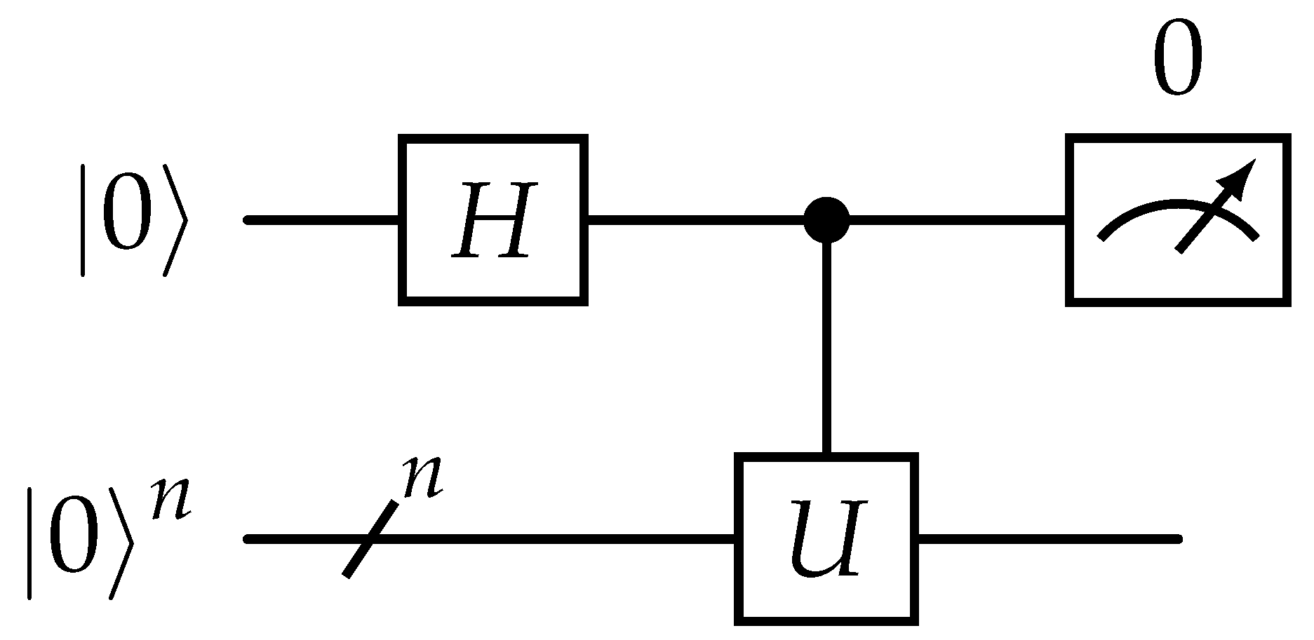
U conditionally on a target-qubit register, if a control-qubit has a |1〉 component. An example of a multi-qubit, controlled gate is illustrated in
Figure 2, where the first qubit acts as control-qubit and the rest
n qubits as targets.
2.2. Quantum Linear System Problem
When given a Linear System Problem (LSP) of
N linear equations and
N unknowns which can be expressed as
, where x is the vector of unknowns,
A the matrix of coefficients and
b is the right-hand side vector, one can construct the Quantum Linear System Problem (QLSP) [
14,
15]
where
is the normalized right-hand side and
A the normalized matrix satisfying
.
Although QLSP is practically a normalized version of the LSP, they are two distinct problems with latter being addressed mostly by quantum algorithms. The main difference is the requirement that both the input and output of a QLSP are given as quantum states. This means that any efficient algorithm for QLSP requires an efficient preparation of |b〉 and efficient readout of |x〉, both of which are open problems for the general case.
In the quantum linear systems algorithm literature, the term "efficient" usually refers to polylogarithmic complexity w.r.t the system size
N. This means that Quantum algorithms like [
16] solve the QLSP exponentially faster than even the fastest classical algorithms like Conjugate Gradient method. Solving and reading in quantum computing, though, are two completely distinct processes and as such, we must note though that in order to read out all the elements of |
x〉, we would still require
time, just as any efficient classical algorithm. Hence, a solution to QLSP should be used as a subroutine in an application where
samples from vector
x are useful, as discussed thoroughly in [
17].
3. The VQLS algorithm
The Variational Quantum Linear Solver (VQLS) [
10] is a Variational Hybrid Quantum-Classical (VHQC) algorithm used for solving QLSPs and designed with NISQ devices in mind. Given the QLSP
, the quantum part of the algorithm uses a cost function which captures the similarity between vectors
and |
b〉, by means of either a local or global Hamiltonian. Classical optimization schemes can be then utilized in order to minimize the Hamiltonian loss and finally terminate when a desired precision
is reached.
Although variational algorithms are heuristic and complexity analysis of VQLS is a challenging open problem, the authors of [
10] provided numerical simulations indicating efficient scaling in the linear system’s dimension
N, condition number
and desired absolute error
w.r.t the exact solution. Specifically, they found evidence of (at worst) linear scaling in
, logarithmic scaling in
and polylogarithmic scaling in
N [
10].
3.1. Overview
The algorithm requires the following as input: an efficient operator initializing a quantum state
, a vector of initial parameters
and a linear decomposition of the normalized matrix
, with
being unitary matrices and
. Intuitively, this linear decomposition into unitaries is essential to construct the required circuits since all quantum gates are unitary operators themselves. VQLS requires the following assumptions be made:
L scales as
,
A has a finite condition number
, its spectral norm satisfies
. The
unitaries must additionally be implemented with efficient circuits, which in quantum computing terms, this usually implies a worst case polynomial dependence on
n. Information over efficient decomposition method for sparse
A can be found at [
10]. The output is the quantum state |
x〉 that approximately satisfies the system
up to a constant factor. Parameters
in the ansatz
are adjusted in a hybrid, quantum and classical optimization scheme until the cost
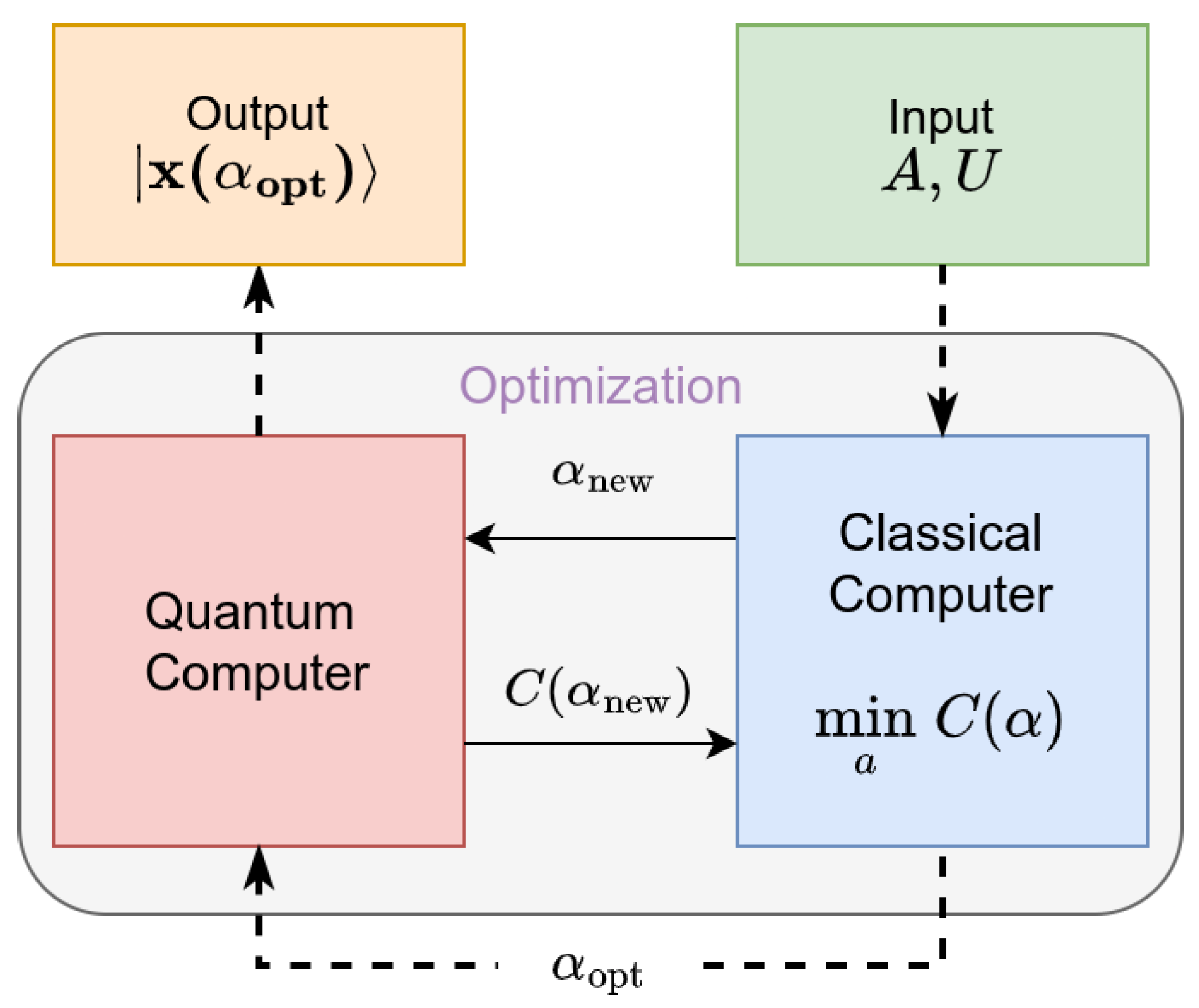
(local or global) reaches a predefined threshold. Lastly, the optimized ansatz is applied to construct the solution state which may be measured in order to compute observable quantities of interest. An overview of the algorithm can be seen in
Figure 3.
As mentioned, in order to solve the QLSP one must prepare a state |x〉 s.t. is as close as possible to |b〉. In order to achieve that, VQLS employs an ansatz that prepares a candidate solution . A parameter vector is given as input to the quantum computer, which prepares and runs an efficient quantum circuit that estimates a cost function . The cost function’s value quantifies how far the proposed state deviates from the desired state |b〉. This value is then returned to the classical computer which adjusts parameters according to a classical optimization algorithm, attempting to reduce the cost. The process is repeated until a termination condition of the form is achieved, at which point VQLS outputs the solution parameters .
Finally, the optimal parameters are given as input to the ansatz which computes the solution state . Once the solution state is achieved we can finally measure quantities of interest in order to extract valuable information for the solution vector. The deviation of observable expectation values from those of the exact solution can be upper bounded based on the cost function.
3.1.1. VQLS Cost functions
According to [
10], the cost functions can be described as expectation values of either global or local Hamiltonians. To avoid cumbersome notation, we will thereafter write
. As it is noted in [
18], global functions may introduce barren plateaus in the energy field, which lead to exponentially vanishing gradients with respect to the number of qubits
n. For improved trainability as
n grows larger, the authors introduce local Hamiltonian, the normalized version of which is
where
is normalized. The effective Hamiltonian is
and
is the zero state on qubit
j and
the identity on all qubits but qubit
j.
3.2. Cost evaluation
In order to estimate the cost
one must evaluate each part of the fraction in Equation
6 separately, with the first and simpler term to evaluate being
where
Also, for
one needs to estimate the terms
where index
j implies application of corresponding operator to the
j-th qubit, while
refers to every other qubit but
j. By exploiting the fact that
,
10 can be written as
where
Taking the previous into account, the cost function finally becomes
where each of the terms
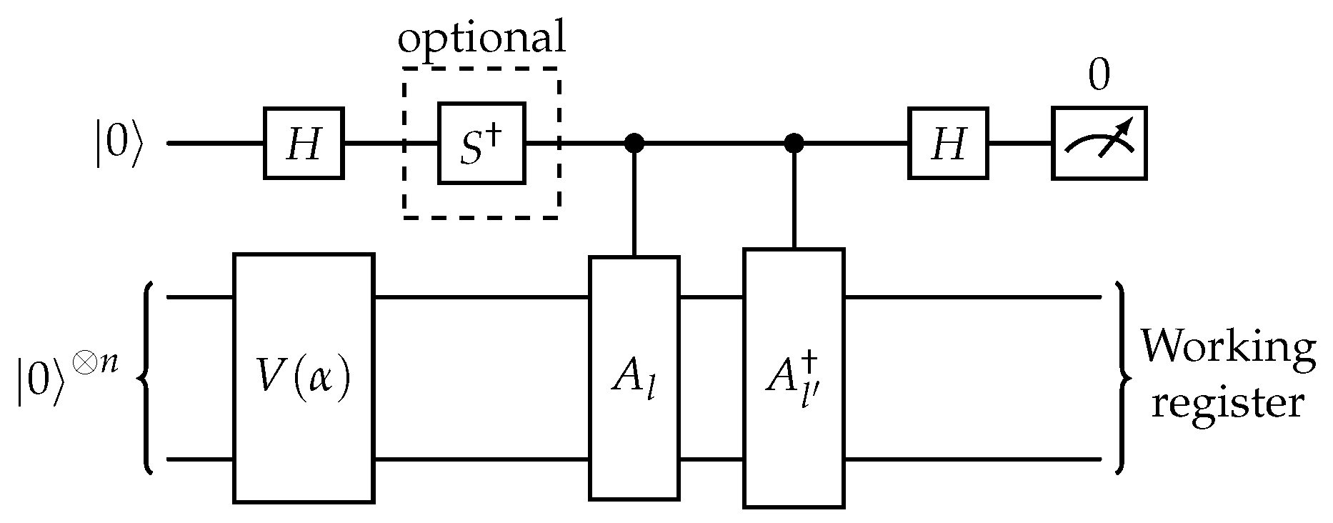
are computed by postprocessing the output of the circuits shown in
Figure 4 and
Figure 5 respectively.
The circuit in
Figure 4 applies operator
V on |
0〉 and then, conditioned on the first qubit, applies two controlled operations,
followed by
. Finally, a measurement takes place in the ancilla circuit. The
gate is added to the circuit when the imaginary part of the expectation value is needed. In a similar manner, the circuit of Figure
10 additionally applies the
,
and
U operators. The case shown corresponds to
, when controlled-
Z gate is applied to first qubit of working register. As before the
gate is added to the circuit when the imaginary part of the expectation value is needed.
3.3. Ansatz
VQLS works by preparing the state
. The unitary operator
consists of a sequence of gates with trainable continuous parameters
and can more or less be expressed as
The discrete parameters
encode the types of gates and their placement in the circuit. Such empirical gate constructs are called ansatzes and are common in variational quantum algorithms in general.
If
k is constant, we are referring to "fixed-structure" ansatz, since one optimizes only over
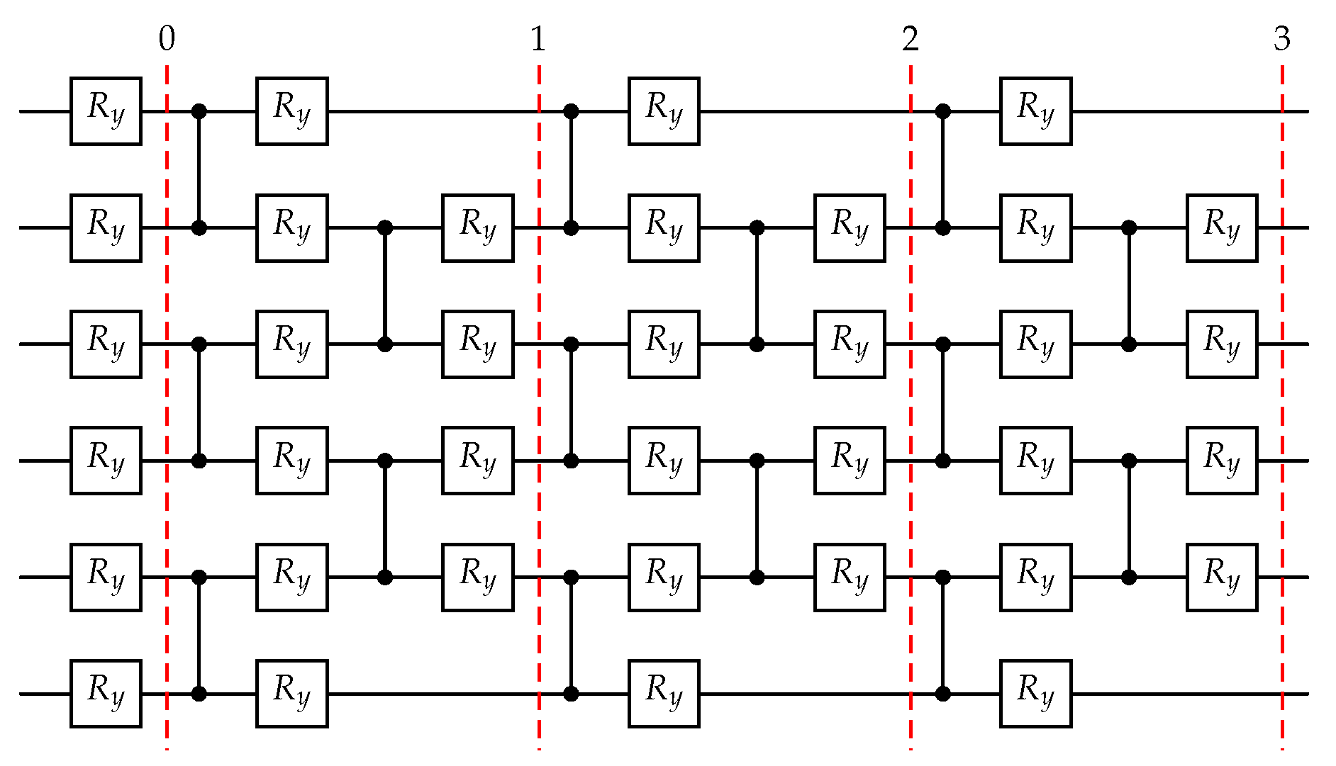
. An example of fixed ansatz can be seen
Figure 6. Although less versatile, fixed ansatzes are simpler than "variable-structure" ones, where one optimizes with respect to
k as well. Lastly, another type that can be employed is the Quantum Alternating Operator Ansatz (QAOA) [
19,
20], which is known to be universal as the number of its layers tend to infinity [
21,
22].
4. AI-VQLS-solver: coupling Quantum Computing with machine
learning to accelerate the solution of parameterized linear systems
In a multitude of applications, such as uncertainty propagation, parameter inference, optimization, sensitivity analysis etc. it is required to produce sufficient number of samples or solution datasets. These, in turn, require the solution of parametric linear systems, and besides the often unavoidable, immense matrix sizes, one has to deal with an overwhelming number of LSP instances which often exceed available computational resources. While quantum algorithms, and specifically VQLS, are expected to deal with the former challenge by exponentially reducing the computational complexity of individual LSPs, there still remains space for further acceleration of the overall parametric problem.
In this regard, it is essential to derive efficient methods that exploit the continuity of the LSP solution space with the respect to the parameters that produce the linear system, hereafter called physical parameters
. Starting from the linear system with equation
, with
being the parametrized system matrix,
x the solution sought and
b the right-hand side vector. The equivalent QLSP is the system with equation
. Finally, when a variational quantum algorithm such as VQLS is used as solver, the system takes the form
where
the VQLS real parameter-vector and
the proposed solution of the QLSP. Using the cost function from Equation
6 the optimal parameters are obtained by the following minimization problem
It is evident from Equation
16 that for every matrix
, a search over parametric space
is required in order to reach the solution
which minimizes the Hamiltonian cost
.
Our proposed scheme uses a machine-learning model in order to propose refined initial guesses to the VQLS algorithm. Instead of letting the initial VQLS parameters be random or constant, we take advantage of the assumed continuity of the cost function , so that for every physical parameter p, a refined initial guess is proposed that is as close as possible to the optimal ones with some probability depending on the chosen model. The acceptable error between the proposed and optimal parameters is a hyperparameter for the overall scheme and depends on the value of the training loss.
Since, in general, no training dataset will be available, one has to initially rely on the usual workflow without refined initial parameter proposition i.e. for using some generic strategy . Once the first optimal solutions are produced, the model can be trained on the respective dataset . The trained model thereafter proposes refined initial parameters for . Again, is considered a hyperparameter which must be chosen to balance the trade-off between accuracy and training-time.
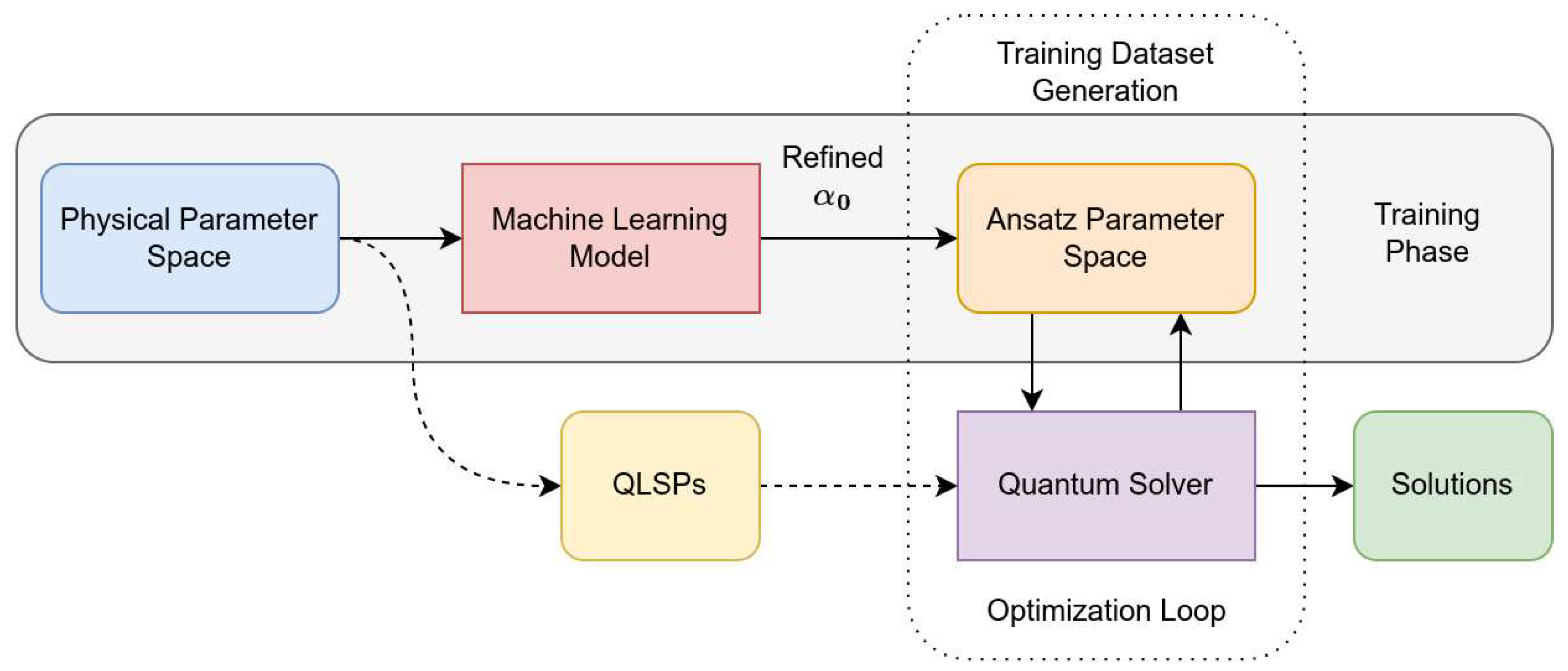
The overall scheme is presented in
Figure 7. Initially, as noted, the scheme follows the dashed arrows generating the training data by solving the first
QLSPs with the base-VQLS. Once the training dataset has been generated, the machine-learning model is trained with
as input and
as output. The computational scheme thereafter changes as indicated by the solid arrows, with the model now proposing refined initial VQLS parameters
, which are closer to the optimal, thus reducing the optimization cost for a QLSP instance.
In the model architecture context, in order to minimize training time without adding to the overall execution time, it is desirable to choose a ML model
with low complexity and efficient scaling with respect to its output. In our scheme, the only hyperparameter that can be controlled in this regard is the complexity of the ansatz
V and more specifically the dimension
r of the ansatz parameter vector
. An ansatz that scales polynomially with the number of qubits is desirable because it enables one to construct models that remain efficient as the size of the system increases. Specifically, in our case
r should scale at most as
, where
n the number of qubits required for the system, so that low-complexity, efficient ML models are sustainable. Some known ansatzes with polynomial qubit scaling include the Quantum Approximate Optimization Algorithm (QAOA) ansatz [
5] and the Hardware-Efficient ansatz [
23].
5. Numerical examples
To evaluate the performance of the proposed scheme we conducted the comparative experiments described in the subsequent section. The quantum circuit simulations were driven by the Qiskit open-source framework and specifically the
statevector simulator [
24]. The matrix generator for the parametric
QLSP is chosen to be
where
n is the number of effective qubits used in the circuit,
are coefficients that depend on the physical parameters
p, while
are normalization constants. In both examples, the physical parameters
are uniformly distributed in a 3-dimensional unit cube
. At each example we compare pure VQLS schemes with ones that fall under our paradigm. Since the circuits are simulated, the comparison is conducted in relation to the required number of iterations to solve each instance of the parametric system. The parametric QLSP is discretized into a total of
regular QLSPs, with equations
and
. For all examples the right-hand side is set to
and the total number of solutions
.
5.1. Convergence and continuity
A main problem when using variational algorithms is that the Hamiltonian loss-functions and especially their local versions are inherently non-convex which increases the probability for different optimization paths with neighboring initial parameters to land astray at completely different local-minima. Furthermore, quantum ansatzes are inherently periodic, since most parametric quantum gates themselves are not bijective with respect to their parameters. In fact, quantum gates are essentially rotations with period of at most and the parameters themselves are rather angles of rotation in some complex Hilbert space. Thus, when an ansatz is deployed, in general there is often a multitude of parameter values that can produce the same state. Besides periodicity, an ansatz contains many different paths through which the quantum states are prepared, resulting in different quantum states that may possess the same properties and more specifically the same probability distribution when measured under a specific basis. Lastly, when dealing with real quantum processors, the unavoidable hardware noise will most definitely propagate through the optimization path resulting again in discontinuous optimal values.
Another source of discontinuities which may arise in low-qubit systems is over-parametrization of the quantum ansatz. The required number of parameters to fully span an
n-qubit system’s Hilbert space is
, whereas the number of parameters of an efficient ansatz usually scales as
. Hence, as
more often than not the optimization problem will be under-parametrized, since
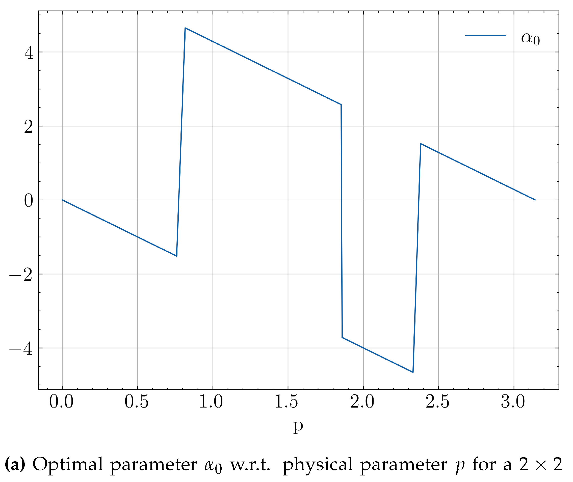
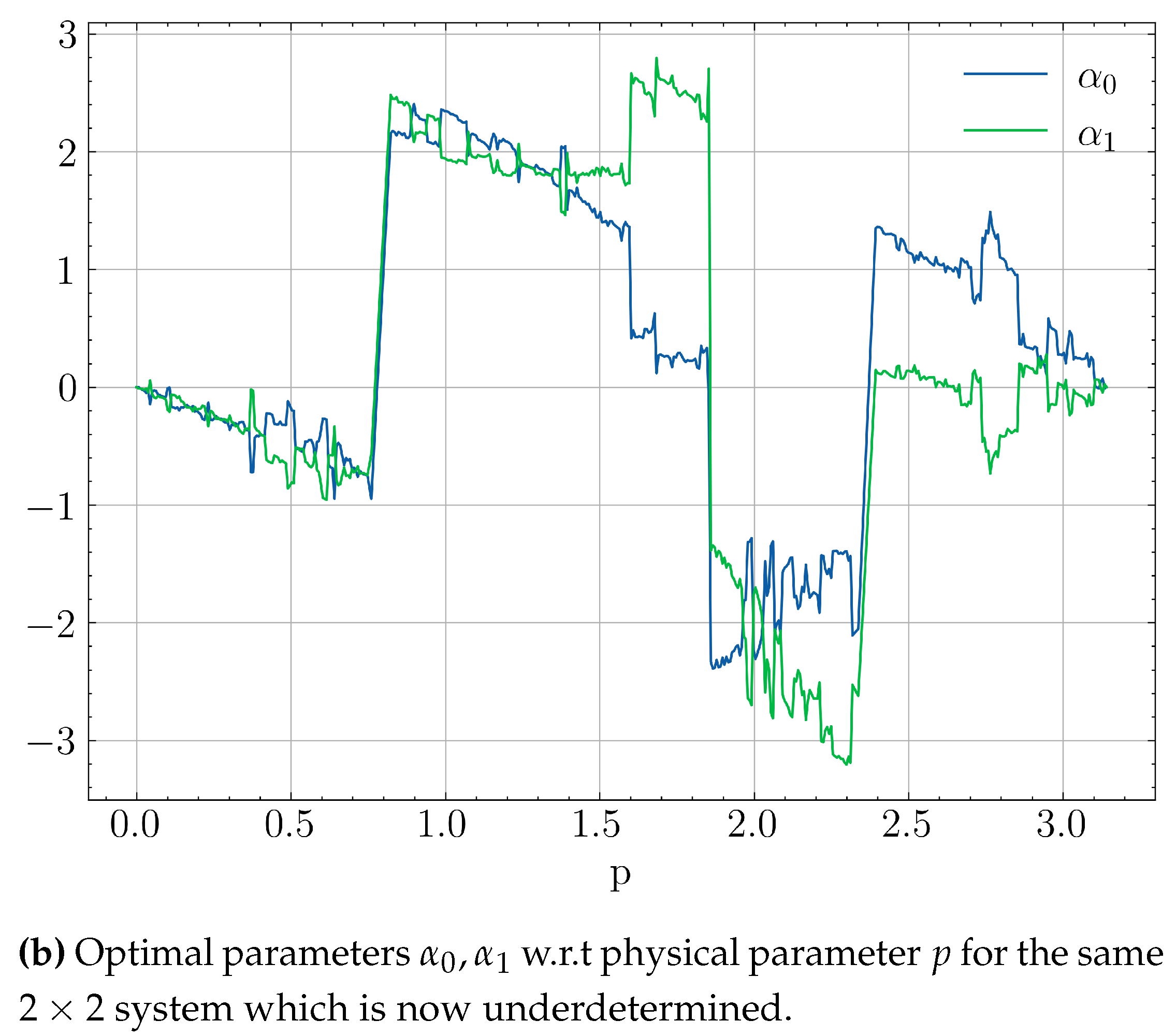
. In smaller systems, though, where the previous inequality is not guaranteed, one might eventually use more parameters than required. This will lead to an underdetermined system with infinite solutions w.r.t a portion of its parameters, giving optimizers more paths to explore, but also more ways to diverge from previous strategies. A the simple illustrative example of this behaviour can be seen in
Figure 9. The discontinuities in
Figure 9a are due to the periodicity of the non-convex Hamiltonian loss which allow jumps between different local minima. In
Figure 9b which has more than required ansatz parameters, the system becomes underdetermined resulting in more discontinuities.
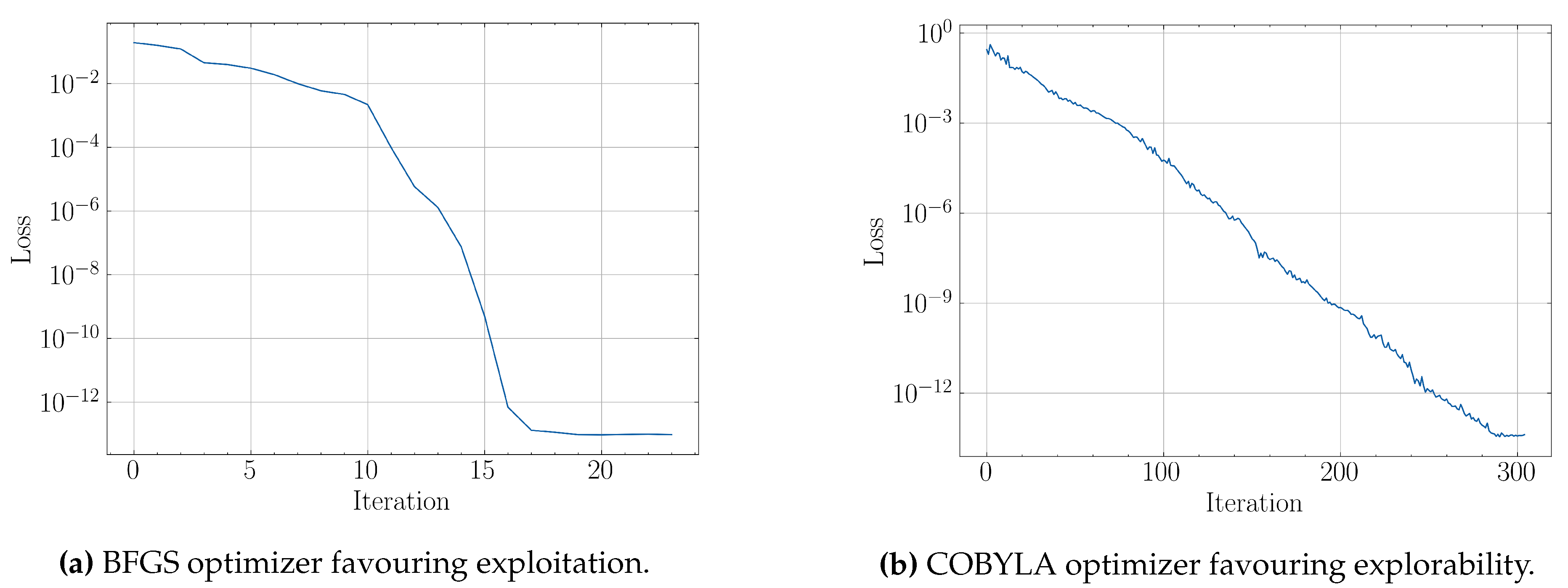
From the above, it is apparent that in order to ensure precision and suffice to simple, scalable model architectures, it is imperative to take into account any potential hindrances posed by aforementioned discontinuities, which can obstruct training and prediction to a substantial extent. Coherently, various classical optimizations schemes used in VQLS may introduce different convergence behaviours with respect to the utilized algorithm. When dealing with convergence alone, the only optimization property that matters is the execution time, where the fastest algorithm to reach a minimum loss, can be considered best for the given problem. In our case though, continuity is of equal importance, since we seek to not only reach a solution, but to force systems with close physical parameters to produce output in the ansatz parameter space in the same neighbourhood. An optimization algorithm that favours explorability instead of exploitation has a higher chance to visit different local minima during the optimization of concurrent, similar QLSPs and thus resulting in optimal parameter discontinuities with higher probability. In the subsequent experiments, we were confined to gradient-free optimizers in order to evaluate their sufficiency with respect to the potential discontinuities.
5.2. Example 1: two-qubit system
The first example consists of the QLSP in Equation
17 for
, which results in a parametric system of size
, with the coefficients
chosen as trigonometric functions of the physical parameters
e.g.
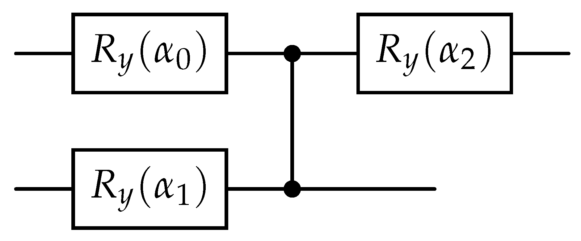
. For the solution of the QLSPs a BFGS optimizer was used with numerical first and second order derivatives approximation. The ansatz used in the example is shown in
Figure 10
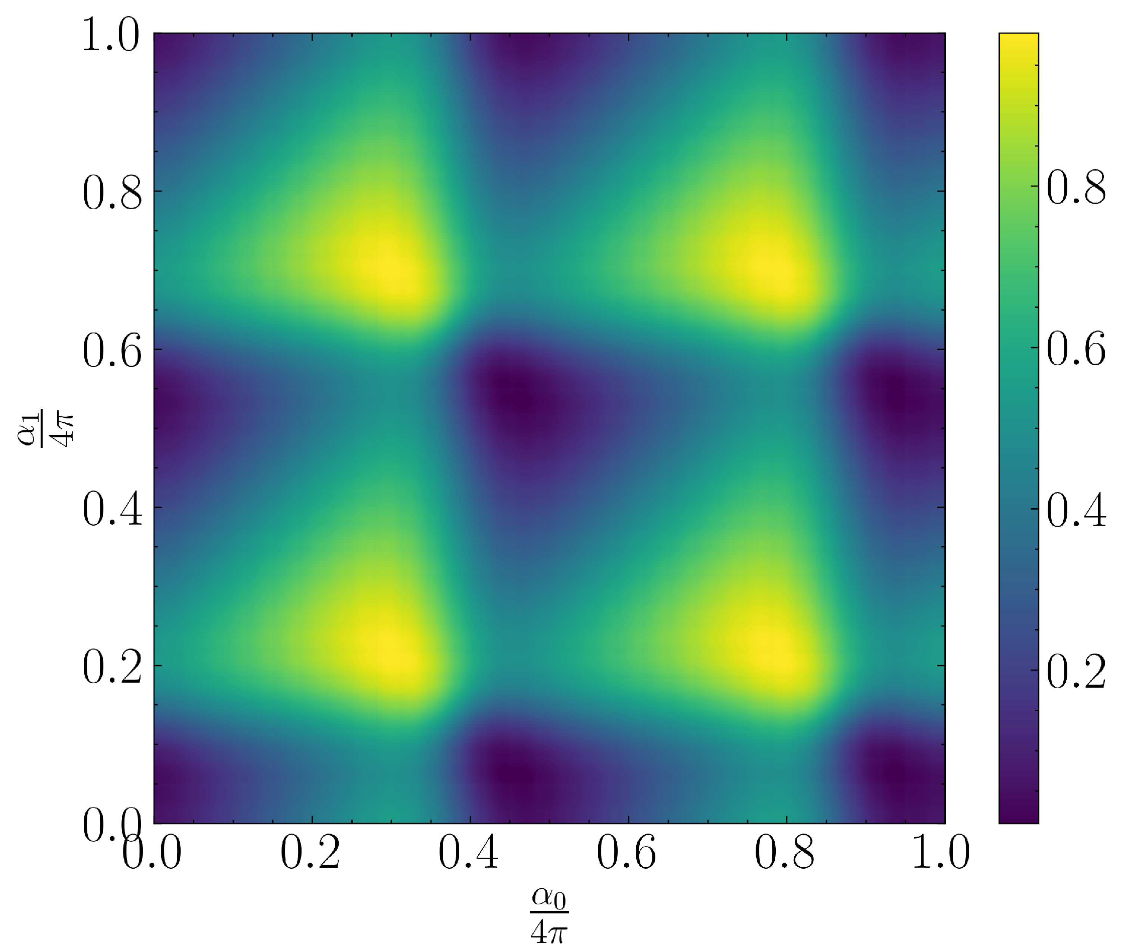
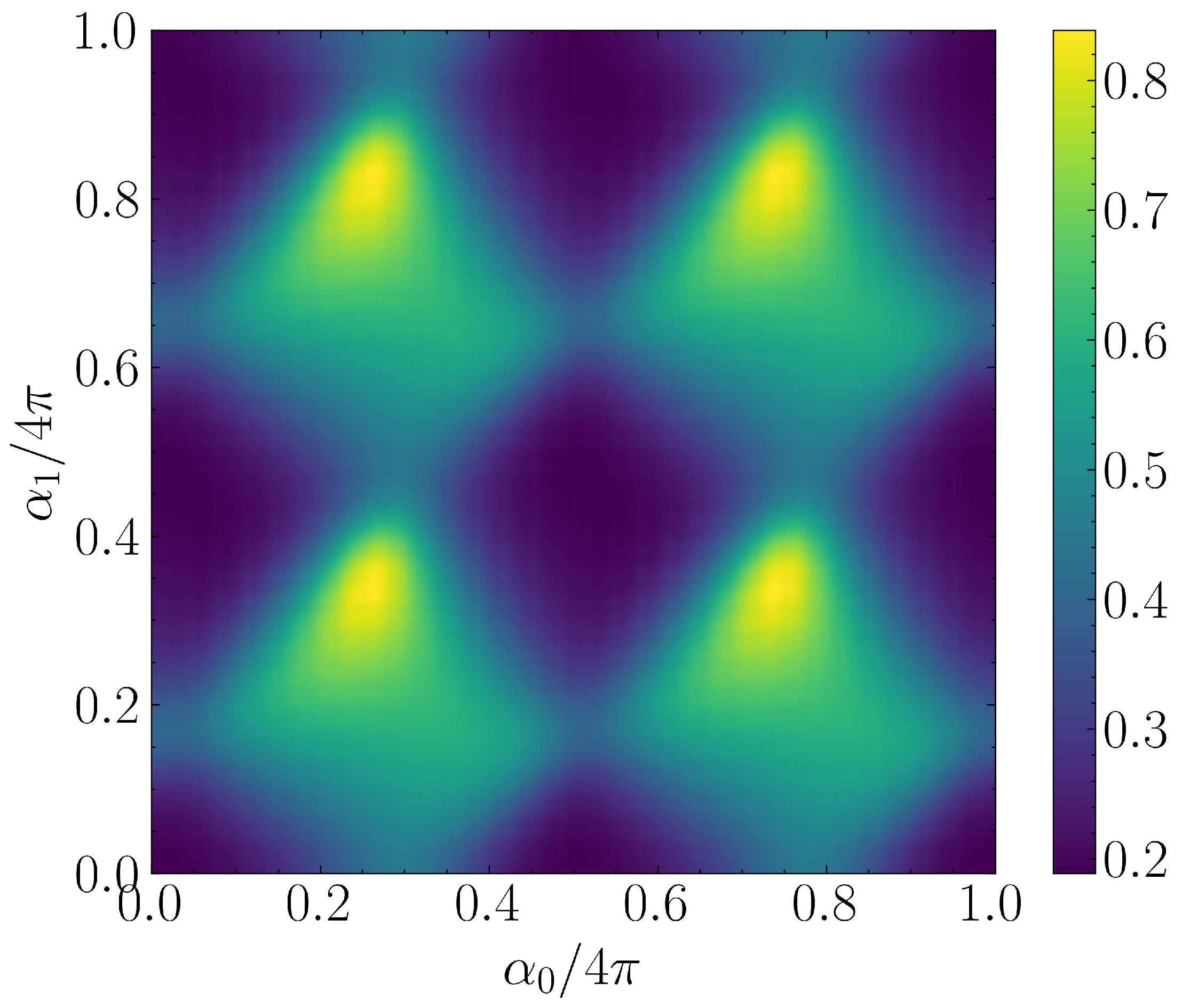
The Hamiltonian cost function for a given QLSP instance can be seen in
Figure 11. We observe an intensive non-convex behariour and periodicity resulting in different local minima which may have hindered optimization algorithm to consistently extract continuous optimal solutions
across all QLSP instances.
In this example, three strategies were implemented: in the first two the basic VQLS scheme was used with constant, , and uniformly random, , proposed initial parameters respectively, while the third strategy consists of a naive nearby scheme, where the proposed initial parameters for each linear system were the optimal parameters of the previous one . The nearby strategy requires an initial reordering of the QLSPs w.r.t the dimensions of the physical parameters. The latter strategy takes advantage of the continuity of the QLSP and requires that are mostly sorted at each dimension in order to avoid large gaps between the sought optimal ansatz parameters. This scheme is quite efficient in the sense that it does not require any training, , prior to its application and can be compared in a direct manner with the base VQLS.
In
Figure 12 one can see the joint probability distributions of the optimal parameters
for
,
for the
example of this section. In this example the dataset had no discontinuities which led to a trainable ML model.
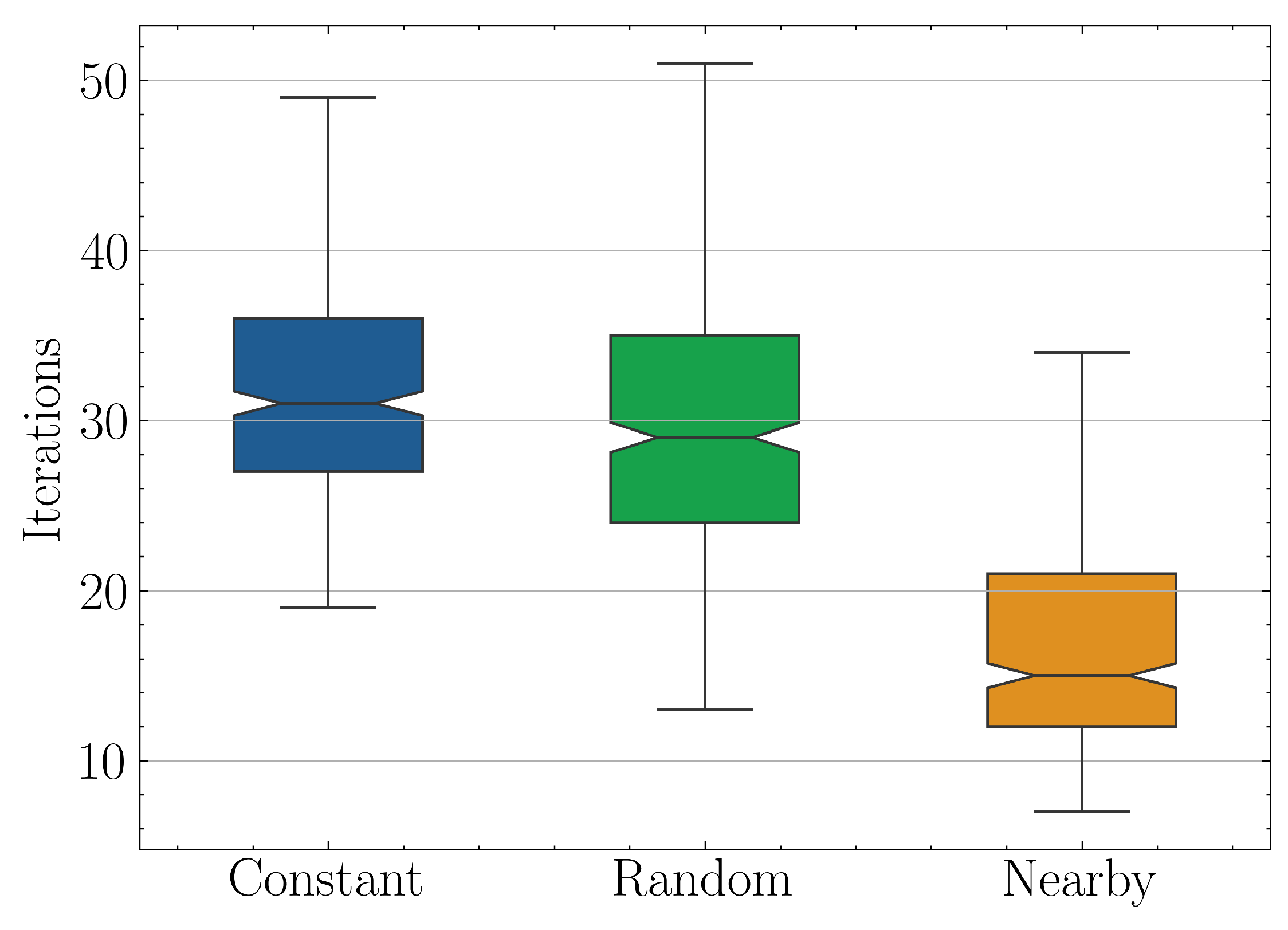
The comparative results of the three strategies can be summarized in
Figure 13, where the required iterations distribution for solving one instance of the parametric QLSP
are shown. On the left is the pure-VQLS scheme with constant initial ansatz parameters, in the middle a similiar approach but with random initialization and on the right the naive nearby approach, where the proposed ansatz parameters for each system is taken as the optimal of the previous. The speedup factor of the latter over first two schemes based on their median values is
.
5.3. Example 2: three-qubit system
For the second example, a three-qubit system was chosen, which results in a parametric system of size
, with the coefficients
being polynomial functions of the physical parameters
e.g
. For the solution of the QLSPs a BFGS optimizer was used with numerical first and second order derivatives approximation. The 2-layered ansatz used for this example takes as input a vector
. Each angle
is used as a parameter for the
gates which are structured as shown in
Figure 14. For the solution of the systems a BFGS optimizer was used with numerical first and second order derivatives approximation.
Three distinct strategies were compared, the first two are the pure VQLS scheme with constant initial parameters and the naive nearby scheme, as before. Additionally, as a third approach a simple MLP with 2 hidden layers was trained in the first
samples using standard MSE loss and an Adam optimizer. In contrast to the nearby scheme, the optimal parameters used for training must cover the whole solution space in order to better approximate the manifold they reside in. In
Figure 15, one can observe the non-convex Hamiltonian cost function
for an instance of the QLSP. As in the first example, the Hamiltonian is non-convex resulting in different local minima, each one with similar loss values. This behaviour is expected when using local cost functions
.
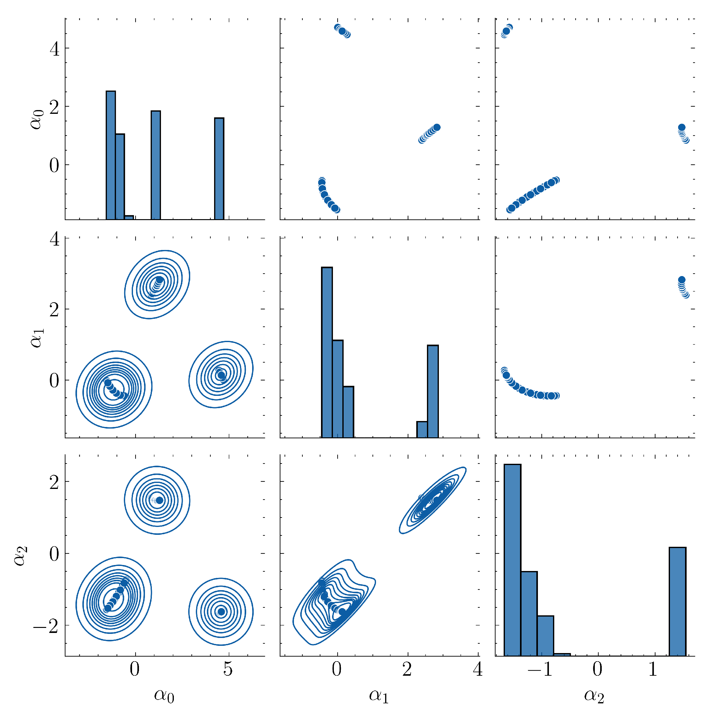
In
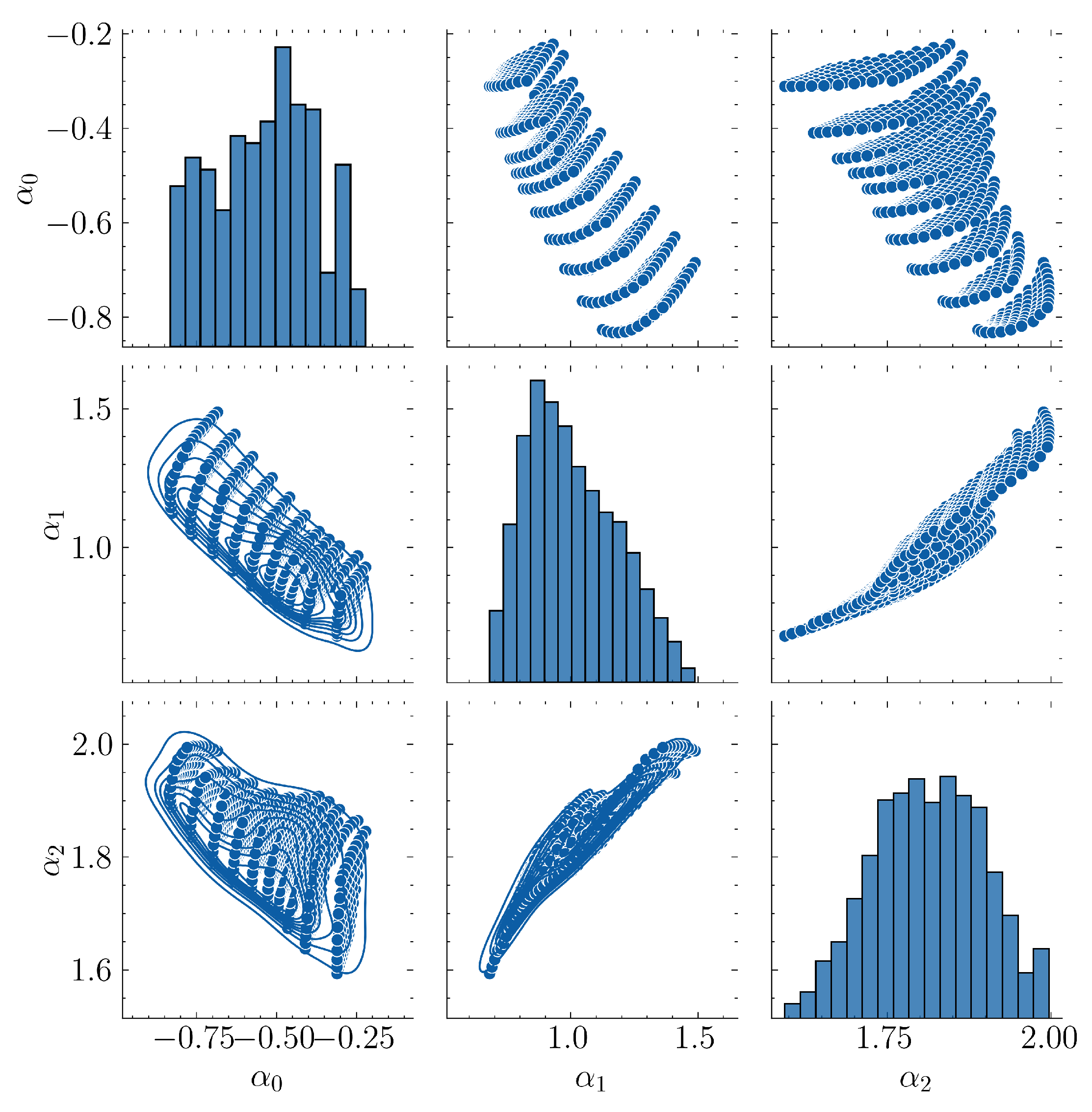
Figure 12 one can see the joint probability distributions of the optimal parameters
for
and
for the
example of this section. In this example the dataset had no discontinuities which led to a trainable ML model.
Figure 16.
Pairwise joint probability distributions of optimal parameters
for example
5.3. In this example there are no discontinuities resulting in easier training of ML models.
Figure 16.
Pairwise joint probability distributions of optimal parameters
for example
5.3. In this example there are no discontinuities resulting in easier training of ML models.
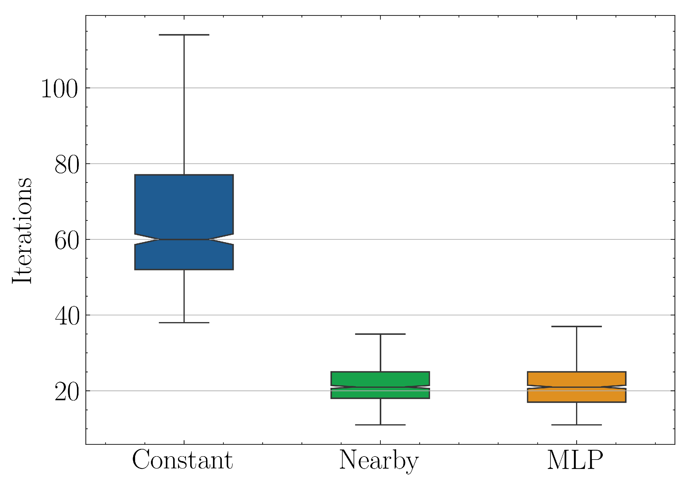
The numerical results of the three strategies Constant, Nearby and MLP, are summarized in
Figure 17. For each strategy, the graph shows the quartile distribution of the number of BFGS iterations required to reach a minimum Hamiltonian loss of at least
for a given QLSP instance. The last two strategies seemingly provide the same level of acceleration with speedup factor over the original algorithm being
based on the median values. However, the MLP model didn’t outperform the naive Nearby method, since the mean square error, after an initial drop, usually was trapped in plateaus which were difficult to overcome without hyperparameter fine-tuning. Due to the fact that our experiments were simulated and did not include QPU runtimes, which are directly comparable to the time spend in fine-tuning, we were forced to be quite conservative with the latter. To our knowledge, unless one can use real quantum hardware and time metrics, it is not apparent how to take into account and compare the required MLP training time with respect to overall VQLS iterations. The assumption eventually made was that by using scalable models and as
, which is the field quantum algorithms are supposed to excel, the model training time will be negligible with respect to the total solution time since
.
Regarding the low MLP performance, it seems that in order to outperform a naive nearby approach in such a small scale, a very delicate fine-tuning of the undermine the predictive ability of simple models played the most important role. Furthermore, the majority of the optimized parameters dataset cannot be used for training, as is common practice, since increasing the training data means that more solutions will be generated using the base VQLS scheme which is slower.
6. Conclusions and future work
Variational algorithms — specifically in our context VQLS algorithm — are designed for the noisy qubits of the current NISQ era. In order to solve the QLSP, VQLS optimizes classically a parametric ansatz w.r.t a quantumly computed Hamiltonian cost function.
Our proposed machine-learning scheme aims to accelerate the convergence of variational quantum algorithms when they are utilized as solvers in parametric problems by taking advantage of continuity. As a proof of concept, we showed that there is potential in that direction, since we managed to achieve a speed-up factor of up to 2.9. In the studied cases, the nearby shceme which combines both speed-up and simplicity seems to be preferable. We also demonstrated that when using gradient-free solvers, and especially ones which favour explorability, discontinuities in the optimal ansatz parameters emerge for various reasons, most prominently due to non-convexity of Hamiltonian loss and periodicity of quantum ansatzes w.r.t. their paramaters. This considerably handicaps the performance of machine learning models such as MLPs, a problem that should be addressed in the future in order to take full advantage of modern ML models.
A natural next step in order to overcome those hindrances is to use exact gradient-informed optimizers, which shall favour exploitation over exploration of parameter-space. Additionally, using domain constraint optimizers will help alleviate discontinuities related to the periodicity of the Hamiltonian. In particular, the use of natural gradient methods initially proposed in [
25] for classical neural networks and their quantum counterparts [
26] may provide sufficient robustness to the optimation process and in this way addressing the discontinuities originating from non-convex loss functions. An extensive evaluation of transformation-preprocessing techniques may also help significantly in this regard. Without doubt, increasing the scale of the experiments will allow bigger training datasets, which will in turn enable more complex, deeper machine learning models to be trained. Finally, experiments with real quantum hardware noise must be conducted so that similar obstructive phenomena are highlighted and addressed.
Author Contributions
Conceptualization, I.K. and K.A.; methodology, K.A.; software, K.A.; validation, I.K.; formal analysis, K.A.; investigation, K.A.; resources, G.S.; data curation, K.A.; writing—original draft preparation, K.A. and I.K.; writing—review and editing, G.S. and V.P.; visualization, K.A.; supervision, I.K. and V.P.; project administration, V.P.; funding acquisition, G.S. All authors have read and agreed to the published version of the manuscript.
Funding
This research was funded by the European Regional Development Fund of the European Union and Greek national funds through the Operational Program Competitiveness, Entrepreneurship and Innovation, under the call “RESEARCH–CREATE–INNOVATE“ project code: T2EDK-03206 Materialize.
Institutional Review Board Statement
Not applicable.
Informed Consent Statement
Not applicable.
Data Availability Statement
Research data can be shared after justified request.
Conflicts of Interest
The authors declare no conflict of interest.
Abbreviations
The following abbreviations are used in this manuscript:
| QC |
Quantum Computing |
| QPU |
Quantum Processing Unit |
| CSE |
Computational Science & Engineering |
| MLP |
Multi-Layer Perceptron |
| NISQ |
Noisy Intermediate-Scale Quantum |
| (Q)LSP |
(Quantum) Linear System Problem |
| BFGS |
Broyden–Fletcher–Goldfarb–Shanno |
| HHL |
Harrow-Hassidim-Lloyd |
| VHQC |
Variational Hybrid Quantum-Classical |
| QAOA |
Quantum Alternating Operator Ansatz |
| QAOA |
Quantum Approximate Optimization Algorithm |
| VQE |
Variational Quantum Eigensolver |
| VQLS |
Variational Quantum Linear Solver |
| IBM |
International Business Machines |
References
- Shor, P.W. Polynomial-Time Algorithms for Prime Factorization and Discrete Logarithms on a Quantum Computer. SIAM Review 1999, 41, 303–332. [Google Scholar] [CrossRef]
- Grover, L.K. Quantum Computers Can Search Arbitrarily Large Databases by a Single Query. Phys. Rev. Lett. 1997, 79, 4709–4712. [Google Scholar] [CrossRef]
- Harrow, A.W.; Hassidim, A.; Lloyd, S. Quantum Algorithm for Linear Systems of Equations. Phys. Rev. Lett. 2009, 103, 150502. [Google Scholar] [CrossRef] [PubMed]
- Xin, T.; Wei, S.; Cui, J.; Xiao, J.; Arrazola, I.n.; Lamata, L.; Kong, X.; Lu, D.; Solano, E.; Long, G. Quantum algorithm for solving linear differential equations: Theory and experiment. Phys. Rev. A 2020, 101, 032307. [Google Scholar] [CrossRef]
- Farhi, E.; Goldstone, J.; Gutmann, S. A Quantum Approximate Optimization Algorithm Applied to a Bounded Occurrence Constraint Problem, 2014. [CrossRef]
- Farhi, E.; Goldstone, J.; Gutmann, S. A Quantum Approximate Optimization Algorithm, 2014. [CrossRef]
- Schuld, M.; Sinayskiy, I.; Petruccione, F. An introduction to quantum machine learning. Contemporary Physics 2015, 56, 172–185. [Google Scholar] [CrossRef]
- Dunjko, V.; Briegel, H.J. Machine learning & artificial intelligence in the quantum domain: A review of recent progress. Reports on Progress in Physics 2018, 81. [Google Scholar] [CrossRef]
- Havlíček, V.; Córcoles, A.D.; Temme, K.; Harrow, A.W.; Kandala, A.; Chow, J.M.; Gambetta, J.M. Supervised learning with quantum-enhanced feature spaces. Nature 2019, 567, 209–212. [Google Scholar] [CrossRef] [PubMed]
- Bravo-Prieto, C.; LaRose, R.; Cerezo, M.; Subasi, Y.; Cincio, L.; Coles, P.J. Variational Quantum Linear Solver 2019. [CrossRef]
- Huang, H.Y.; Bharti, K.; Rebentrost, P. Near-term quantum algorithms for linear systems of equations with regression loss functions. New Journal of Physics 2021, 23. [Google Scholar] [CrossRef]
- Koczor, B.; Benjamin, S.C. Quantum analytic descent. Physical Review Research 2022, 4. [Google Scholar] [CrossRef]
- Peruzzo, A.; McClean, J.; Shadbolt, P.; Yung, M.H.; Zhou, X.Q.; Love, P.J.; Aspuru-Guzik, A.; O’Brien, J.L. A variational eigenvalue solver on a photonic quantum processor. Nature Communications 2014, 5. [Google Scholar] [CrossRef] [PubMed]
- Childs, A.M.; Kothari, R.; Somma, R.D. Quantum Algorithm for Systems of Linear Equations with Exponentially Improved Dependence on Precision. SIAM Journal on Computing 2017, 46, 1920–1950. [Google Scholar] [CrossRef]
- Dervovic, D.; Herbster, M.; Mountney, P.; Severini, S.; Usher, N.; Wossnig, L. Quantum linear systems algorithms: a primer, 2018. [CrossRef]
- Harrow, A.W.; Hassidim, A.; Lloyd, S. Quantum Algorithm for Linear Systems of Equations. Phys. Rev. Lett. 2009, 103, 150502. [Google Scholar] [CrossRef] [PubMed]
- Aaronson, S. Read the fine print. Nature Physics 2015, 11, 291–293. [Google Scholar] [CrossRef]
- Cerezo, M.; Sone, A.; Volkoff, T.; Cincio, L.; Coles, P.J. Cost function dependent barren plateaus in shallow parametrized quantum circuits. Nature Communications 2021, 12. [Google Scholar] [CrossRef] [PubMed]
- Farhi, E.; Goldstone, J.; Gutmann, S. A Quantum Approximate Optimization Algorithm, 2014. [CrossRef]
- Hadfield, S.; Wang, Z.; O’Gorman, B.; Rieffel, E.G.; Venturelli, D.; Biswas, R. From the Quantum Approximate Optimization Algorithm to a Quantum Alternating Operator Ansatz. Algorithms 2017, 12, 34. [Google Scholar] [CrossRef]
- Wang, Z.; Hadfield, S.; Jiang, Z.; Rieffel, E.G. Quantum approximate optimization algorithm for MaxCut: A fermionic view. Phys. Rev. A 2018, 97, 022304. [Google Scholar] [CrossRef]
- Crooks, G.E. Performance of the Quantum Approximate Optimization Algorithm on the Maximum Cut Problem, 2018. [CrossRef]
- Kandala, A.; Mezzacapo, A.; Temme, K. Hardware-efficient variational quantum eigensolver for small molecules and quantum magnets. Nature 549, 242–246. [CrossRef] [PubMed]
- Qiskit: An Open-source Framework for Quantum Computing, 2021. [CrossRef]
- Amari, S.i. Natural Gradient Works Efficiently in Learning. Neural Computation 1998, 10, 251–276, [https://direct.mit.edu/neco/article-pdf/10/2/251/813415/089976698300017746.pdf]. [Google Scholar] [CrossRef]
- Stokes, J.; Izaac, J.; Killoran, N.; Carleo, G. Quantum Natural Gradient. Quantum 2020, 4, 269. [Google Scholar] [CrossRef]
|
Disclaimer/Publisher’s Note: The statements, opinions and data contained in all publications are solely those of the individual author(s) and contributor(s) and not of MDPI and/or the editor(s). MDPI and/or the editor(s) disclaim responsibility for any injury to people or property resulting from any ideas, methods, instructions or products referred to in the content. |
© 2023 by the authors. Licensee MDPI, Basel, Switzerland. This article is an open access article distributed under the terms and conditions of the Creative Commons Attribution (CC BY) license (http://creativecommons.org/licenses/by/4.0/).
