Preprint
Article

Reproducible Quantification of the Microstructure of Complex Quenched and Quenched and Tempered Steels using Modern Methods of Machine Learning

Altmetrics

Downloads

125

Views

59

Comments

0

A peer-reviewed article of this preprint also exists.

Submitted:

08 July 2023

Posted:

10 July 2023

You are already at the latest version

Alerts
Abstract
Current conventional methods of evaluating microstructures are characterized by a high degree of subjectivity and a lack of reproducibility. Modern machine learning (ML) approaches have already shown great potential in overcoming these challenges. Once trained with representative data in combination with an objective ground truth, the ML model is able to perform a task properly in a reproducible and automated manner. However, in highly complex use cases, it is often not possible to create a definite ground truth. This study addresses this problem using the underlying showcase of microstructures of highly complex quenched and quenched and tempered (Q/QT) steels. A patch-wise classification approach combined with a sliding window technique provides a solution for segmenting entire microphotographs where pixel-wise segmentation is not applicable due to the problem of reproducibly creating unambiguous training masks. Using correlative microscopy, consisting of light optical microscope (LOM) and scanning electron microscope (SEM) micrographs as well as corresponding data from electron backscatter diffraction (EBSD), a training dataset of reference states that covers a wide range of microstructures was acquired in order to train accurate and robust ML models. Despite the enormous complexity associated with the steels treated here, classification accuracies of 88.8% in the case of LOM images and 93.7% for high-resolution SEM images were achieved. These high accuracies are close to super-human performance, especially in consideration of the reproducibility of the automated ML approaches compared to conventional methods based on subjective evaluations through experts.
Keywords: 
Subject: Chemistry and Materials Science  -   Materials Science and Technology

1. Introduction

Due to the excellent combination of properties, the ability to selectively adjust the desired properties at relatively low costs, and the high sustainability in its value chain through high recyclability, steel is justifiably one of the most widely used materials of our time. The complexity of microstructures in modern high-strength steels is increasing enormously because of ever higher demands on the material and constant optimization of the manufacturing processes as well as ever tighter tolerances in quality control due to customer demands. Thus, modern steels have a large number of different microstructural constituents, not all of which can be easily distinguished from one another. Reliable analysis and characterization of the complex steel microstructure is essential to establish on the one hand, a well-founded development of new materials accompanied with a substantial quality control, as well as later process-property correlations to better understand the influences of the process parameters on the resulting microstructure and ultimately, on the properties of the material. The status quo of conventional microstructure analysis is still characterized by a high degree of subjectivity, as well as the experience of the respective metallographer, and is clearly limited by the resolution of the methodology used. Thus, the microstructures are usually evaluated only qualitatively, or only rough estimates of the fractions of the microstructural constituents are given. The experts' assessments are also characterized by poor reproducibility and a lack of objectivity. This also depends strongly on the type and quality of the underlying etching method used to observe the steels.
The use of modern computer vision approaches holds enormous potential for serial application in microstructure analysis, especially in the quantitative evaluation of those, which still is subject to a high degree of subjectivity and a lack of reproducibility. Previous publications demonstrate the valuable advantages of machine learning (ML) in microstructural analysis, particularly the increase in efficiency through automation, as well as the associated reproducibility combined with the objectivity, insofar as the ground truth is well-funded.
Stuckner et al. [1] could transfer common deep learning (DL) approaches to successfully segment microstructures based on a large microscopy dataset in general. De Cost et al. [2] were able to distinguish different microstructural image data classes through an image classification approach according to general microstructural classes, such as brass, different types of cast iron and hypoeutectoid steel, among others. More specifically in case of steels, Azimi et al. [3] could implement a sophisticated approach in order to segment more complex microstructures: They succeeded in performing a pixel-wise segmentation approach using a fully connected neural network (FCNN) in dual phase steels with the aid of correlative microscopy using light optical microscope (LOM) and scanning electron microscope (SEM) images. The final model was able to successfully and robustly segment the matrix as well as the second phase based on microscopic images and identify the second phase object according to the distinguished classes martensite, tempered martensite, bainite and pearlite. Müller et al. [4] extended this classification approach and further differentiated between very complex bainite subclasses. There, morphological features, as well as textural features were used in a traditional ML approach. In case of even more complex segmentation problems, UNets which originally were developed in order to segment medical images [5], could show their superior performance on microstructural images. Through a sophisticated approach, correlative electron backscatter diffraction (EBSD) measurements could help to create objective ground truths in the form of annotated masks to train UNets for semantic segmentation. Here, Durmaz et al. [6] succeeded in training the complex features of lath-shaped bainite to a DL model capable of separating it from polygonal ferrite.
Work on ML-based classification approaches for quenched steels is still limited to date. Tsuitsui et al. [7] used specially heat-treated low-carbon steels to classify entire types of microstructures using SEM images with the aid of texture-based information in the form of Haralick features. A similar approach was followed by Zhu et al. [8], who compared classification based on textural features using conventional ML with DL approaches in the form of a convolutional neural network (CNN) for feature extraction. Bachmann et al. [9] succeeded in using EBSD reconstructions to automatically create masks for an efficient and reproducible segmentation of prior austenite grain boundaries (PAGB) based on Nital-etched microstructural images of quenched steels using only optical microscopy. The authors have no knowledge of other approaches that aim at a direct multiclass segmentation of entire microstructural images, neither on the basis of LOM, nor SEM images of quenched or quenched and tempered steels. This would be of great added value for quality control and microstructure-based process development of these complex steels.
The steels investigated in this work are quenched, as well as quenched and tempered steels with low carbon contents. This type of steel is characterized by a particularly high degree of complexity since the constituents of the steel often differ morphologically only in very fine features. The most common phases found in quenched and tempered steels are martensite, tempered martensite, lower bainite, and partially upper bainite, illustrated in Figure 1.
Martensite is formed during cooling from the high-temperature phase austenite at very high cooling rates. The cooling rate required for martensitic transformation depends mainly on the chemical composition of the steel. Martensite is identifiable by its plate/lath-like structure. Due to the diffusionless and displacing character of the martensitic transformation, the carbon has no time to diffuse or to precipitate in the form of carbides, but is forcibly dissolved within the solid solution, leading to a tetragonal distortion of the cubic lattice [10]. The individual martensite laths can be identified with the help of the clearly pronounced topographical differences after contrasting.
Tempered martensite is formed by tempering processes within the martensite. This tempered state can be created either by an annealing process adjacent to the cooling step, or by self-tempering effects due to residual heat within the material during the cooling process itself [11]. During the tempering, the trapped carbon precipitates from the tetragonally distorted lattice by temporarily allowed diffusion in the form of carbides, which represents its main distinguishing criterion to conventional martensite.
Bainite formation exhibits both a diffusion-controlled and a displacive character [12]. Thus, it also forms at cooling rates intermediate between those of martensite and those of fully diffusion-controlled pearlite. Lower bainite is constituted of lath-shaped featureless ferrite with cementite precipitated within the ferrite laths. The upper bainite is composed of similar lath-like ferrite with continuous cementite precipitates at the boundaries of the laths. Hereby, the cooling rate of lower bainite is higher than the cooling rate at which upper bainite forms. The resulting more restricted diffusion is thus responsible for the different appearances of cementite precipitation within the different bainitic phases. For the sake of simplicity and clarity no further subdivision, as seen in [4], is used in this study investigating complex Q/QT steels.
Figure 1. Schematic Illustration of the morphology of the common microstructural constituents (martensite & tempered martensite – modified acc. to [13], and upper and lower bainite – modified acc. to [14] in Q/QT steels.
Preprints 78969 g001
Despite the different microstructure development mechanisms, all these different phases can occur simultaneously within a microstructure in industrial plates. The main reasons for this are the limited thermal conductivity associated with high material thicknesses and chemical irregularities such as segregation leading to inhomogeneous critical cooling rates along the plate thickness. For the reproducible characterization of these highly complex microstructures, a precise identification of the fine differences is required to identify the present phases.
The biggest obstacle in applying computer vision approaches to the field of materials science is establishing a representative and objective ground truth. In every of the aforementioned works, it was possible to create appropriate training masks with the help of corresponding domain expertise, as well as correlative microscopy, if necessary. This allowed DL models to be trained in order to be able to apply the learned knowledge to unseen images and segment them entirely.
Unfortunately, this is not readily possible with the complex microstructures of Q/QT steels. Even based on the high-resolution SEM images, there are many regions where a clear and doubtless assignment to a class is not possible. The identification of the boundaries between the different structural components is particularly complex, as they frequently merge into one another. This is due to the formation process of the microstructure components. Diffusion in quenched steels is strongly limited and even small differences in local chemical composition have a significant influence on the microstructure development.
Furthermore, the characteristic morphological features of the different phases are mostly, if at all, only visible in high-resolution images. These include the spatial distribution and the shape of the carbide precipitates. Only based on LOM images in most of the cases, even long experienced experts cannot clearly identify these characteristics.
To make the analysis of such complex microstructures more reproducible and efficient, this work aims to combine modern methods of microstructure analysis with promising deep learning approaches from the field of computer vision.

2. Materials and Methods

Material

Due to the high level of complexity combined with a variety of different manifestations of the individual microstructural constituents in QT steels, sample selection is critical to the success of the interdisciplinary approach. In order to cover a sufficient number of features that occur in industrial QT steels, a total of 22 specimens were fully investigated. These include 10 industrial samples from heavy plates taken after being thermo-mechanically treated and 12 dilatometry samples. All samples have a carbon content between 0.16 and 0.22%.
The dilatometry samples were cooled down continuously at different cooling rates (8 – 278ºC) after being fully austenitized at 1000ºC for 10 minutes. In addition, the sample with the highest cooling rate, entirely consisting of martensite, was annealed at 500ºC for 60 min to form reference sections of tempered martensite. Furthermore, other reference samples of the same chemical composition were isothermally cooled to generate additional bainitic reference states. After austenitizing, these were cooled at 50 K/s to the respective holding temperature (425ºC, 475ºC, 525ºC) and held there for a certain time (300 s, or 500 s at 525ºC) and then cooled again at 50 K/s to room temperature. All dilatometry samples used in scope of this study are taken from [4].
The industrial samples were taken from five different heavy plates with thicknesses of 15 mm, 20 mm, 30 mm and 180 mm. The latter was divided into five different samples, in order to map the entire plate thickness. The heavy plates went through different process routes, including direct quenching and conventional quenching and partially, subsequent annealing. In case of direct quenching, the quenching process immediately takes place after the thermomechanical rolling. For conventional quenching, the heavy plate gets time to cool down after rolling before it is heated up again to be quenched [15]. Due to the high material strength of the 180 mm heavy plate and the hereby limited heat transfer, self-annealing effects after the quenching influenced the materials microstructure significantly. Overall, the hereby used materials mainly consist of martensite (M), tempered martensite (MST) and lower (LB) as well as upper bainite (UB).
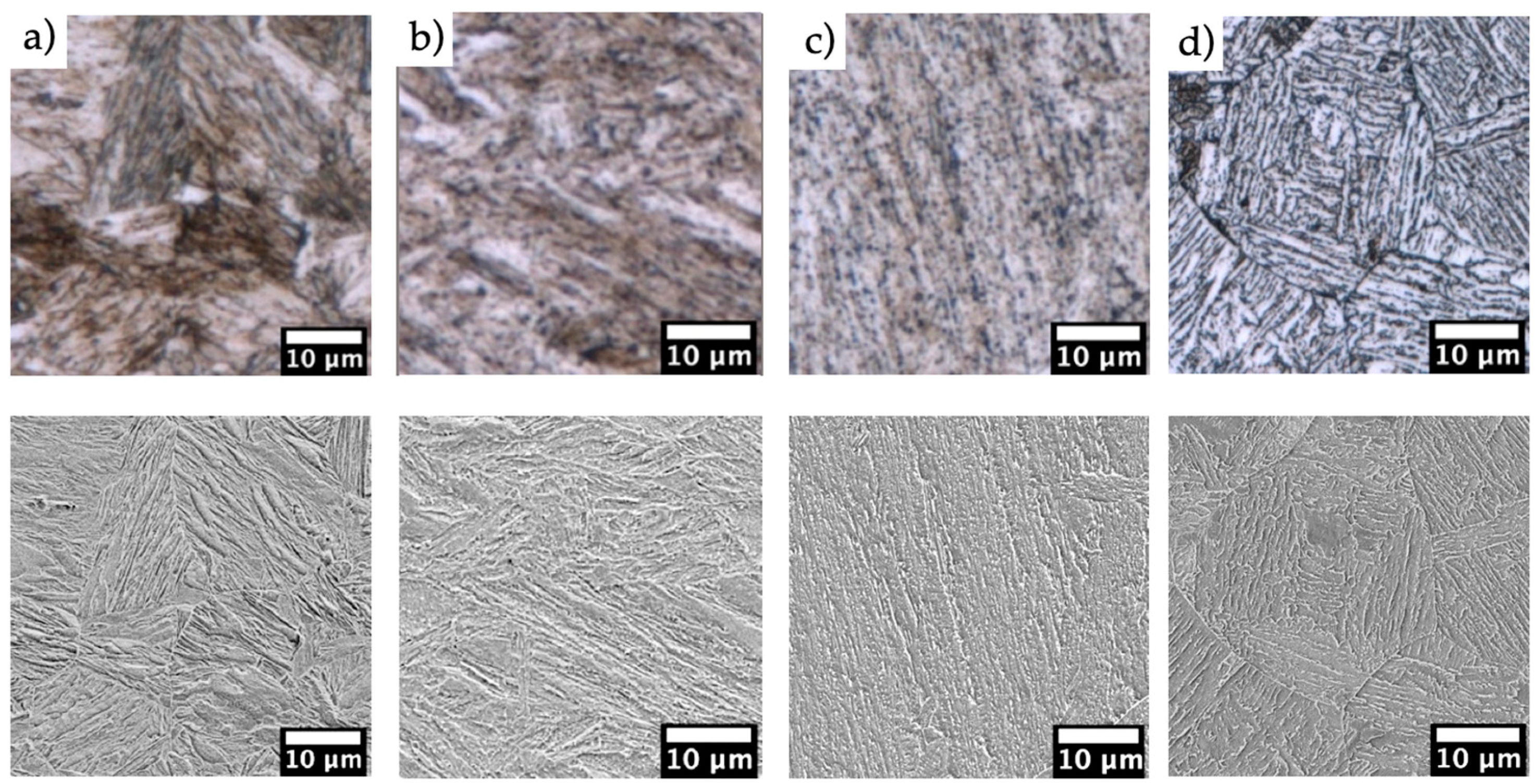
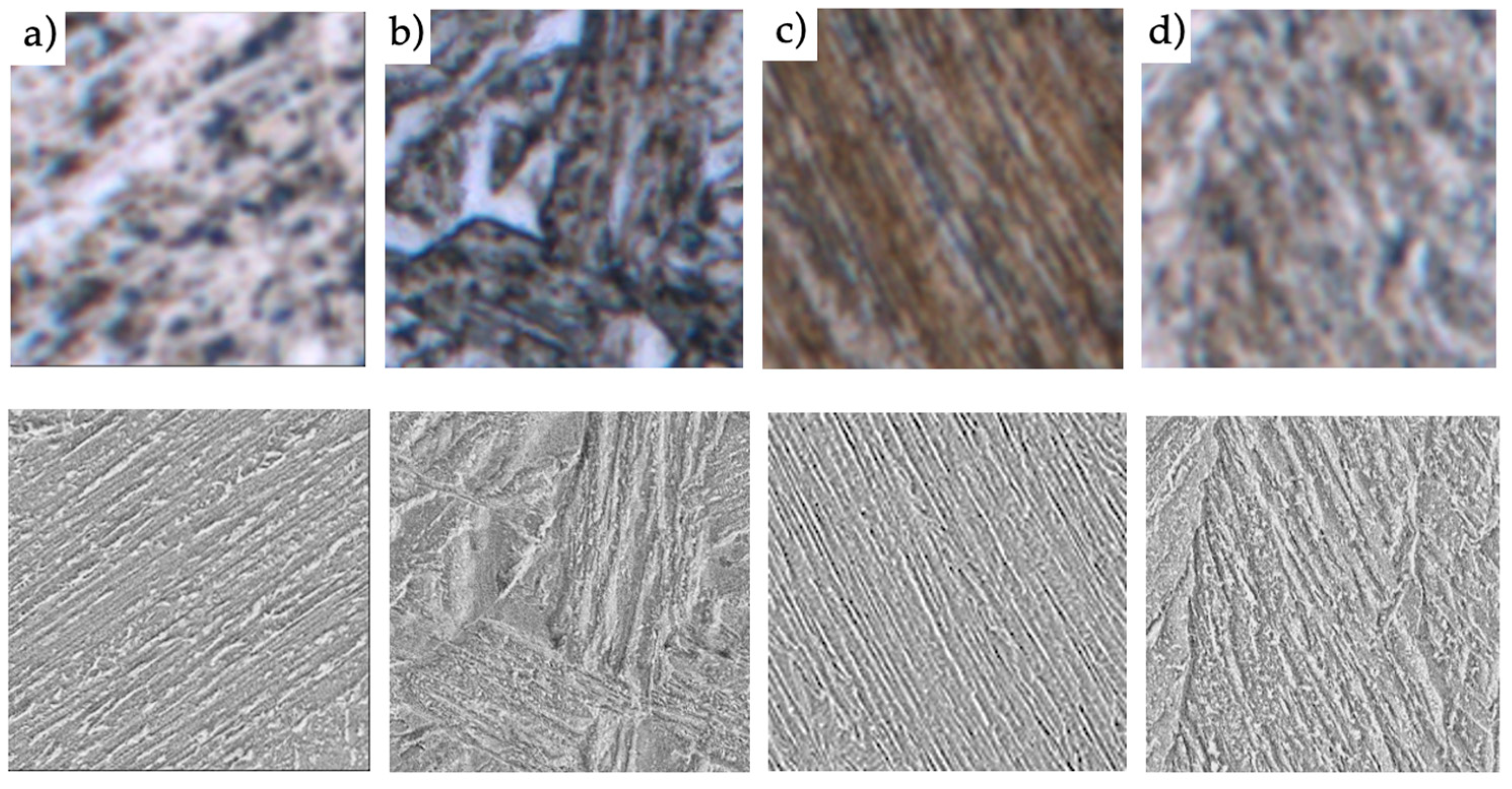
Figure 2 shows respective LOM and SEM images of representative and homogeneous areas of some of the specimens used for this study, illustrating distinct features of the different microstructural constituents. The different colorations in the micrographs are attributed to different phases, originating from different dissolved carbon concentrations, as well as to an orientation influence [16,17] . The high resolution of the SEM images reveals the highly complex features of each phase. Only with the help of those fine details, a clear identification of the different microstructural sections can be made. a) illustrates the significant coloring of a martensitic microstructure in combination with the strongly pronounced topography of the disordered needle structure. MST in b) shows a decrease in coloration due to the tempering process. Nevertheless, the coloration is much stronger than with LB or UB. In the SEM image, the topography and the disordered carbide precipitates can be identified. In the case of the LB c) and the UB d), the ordered lath structure is noticeable. The main focus here is on the differences in the carbide precipitates. In LB, shown in c), the carbon is precipitated in a preferential orientation within the laths in the form of fine carbides. In case of UB, shown in d), coherent carbides form between the bainitic laths.
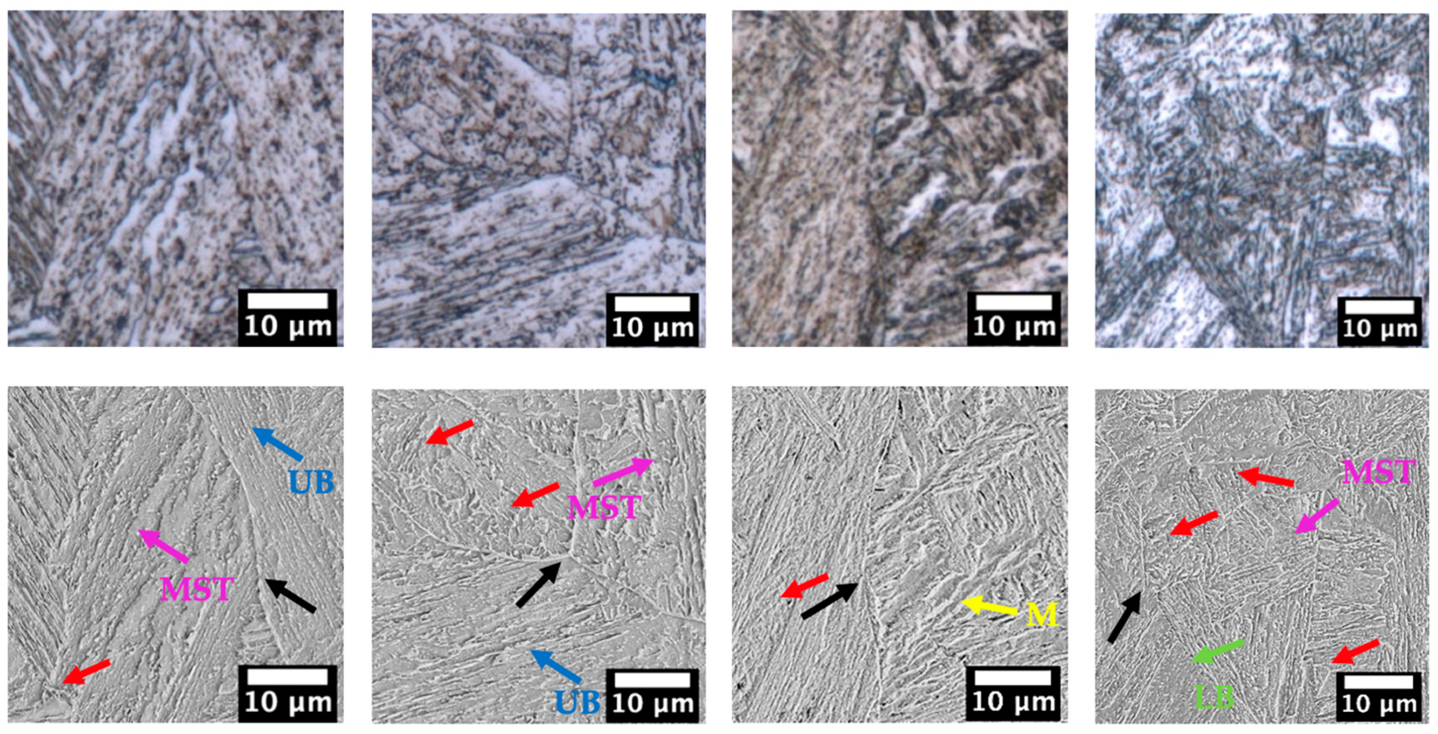
Figure 3, on the other hand, shows areas where a clear identification of the present phases and especially, an identification of the borders between them, is no longer possible without further ado (red arrows). Thus, various sections show characteristic features of different microstructural constituents at the same time. Furthermore, the characteristic areas are extremely diffuse and interwoven, so that no clear boundaries can be drawn. Another problem lies in the multi-layered contrasts of the different microstructural constituents, which are intensified on the one hand by the underlying contrasting technique, which is well known to be limited in terms of reproducibility, and on the other hand by the respective imaging settings of the microscopes.

Correlative Microscopy

In order to guarantee a reliable application of modern DL approaches in the field of material science, high quality data is essential. To establish an objective and well-founded ground truth, it is often not sufficient to limit oneself to a single methodology used for such complex steels, as demonstrated in figure 2 and 3. Therefore, all samples were characterized using LOM, SEM, as well as EBSD. In correlative microscopy, these methods were combined to benefit from the advantages of the different approaches and to eliminate their respective disadvantages and thereby to overcome their limits. In this way, the complementary information necessary for a holistic characterization can be collected on the different length scales and from different contrasting mechanisms. However, the goal behind the correlative microscopy approach is to reduce the actual application to the simplest methodology possible.
All specimens were first ground with 80-1200 grit SiC abrasive paper and then subjected to diamond polishing using 6, 3 and 1 µm suspension. Subsequently, the sample preparation was completed by a colloidal OPS polish to achieve the best possible surface quality for the subsequent EBSD measurement. The respective region of interests (ROI) with a size of 400 x 400 µm, at which the correlative microscopy is being conducted, are marked using hardness indentations.
After each EBSD measurement, which was made on a Zeiss Merlin with an EDAX detector under an accelerating voltage of 25 kV and a beam current of 10 nA at a working distance of 15mm with a step size of 0.35 µm, the sample was briefly polished again using OP-S to remove the contamination layer before further optical examination.
The EBSD data were post-processed with the help of the EDAX OIM software. For this purpose, a standard routine with a filter operation for poorly indexed measurement points was applied.
Subsequently, the samples were contrasted for 25 seconds using a 2.5% alcoholic Nital solution and the micrographs of the respective ROIs were captured in LOM and SEM. As LOM, an Olympus LEXT OLS 4100 laser scanning microscope was used and the images were taken at a 1000x magnification, resulting in a pixel size of 126.6 nm. The SEM images were acquired using a ZEISS Supra SEM using a secondary electron contrast at a magnification of 850x with a respective image size of 2048 x 1536 px corresponding to a pixel size of 47.5 nm. The brightness and contrast settings were adjusted so that the gray level histogram was approximately normally distributed. In order to capture an entire ROI, several single images need to be taken with a respective overlap and subsequently, stitched together. Therefore, Microsoft Image Composite Editor was used.
In order to superimpose the different image data congruently, an image registration is necessary due to the different contrast generation mechanisms as well as unequal perspectives on the respective sample location. For the registration operation the ImageJ [18] Plugin bUnwarpJ [19], as proposed in [16,20] was used. In contrast to their presented procedure, however, the individual features within the different images had to be selected manually. No corresponding features could be found using common automated feature extraction algorithms such as SIFT (=Scale-Invariant Feature Transform), due to the high complexity, as well as the fine visual features of the microstructural images of the investigated steels. First, the high-resolution SEM image was registered on the corresponding image quality (IQ) map of the EBSD measurement. Afterwards, the LOM micrograph was registered on the already registered SEM image.
Another obstacle here is the different resolutions of the individual methods: Either the lower-resolution method must be scaled up and thus interpolated, or important details of the higher-resolution methods may be lost when scaling down. Since the microscopy images are later used in DL algorithms, it is reasonable to adjust, for the sake of simplicity, the image dimensions to powers of 2. Here it is recommended to deviate as little as possible from the native resolutions of the microscopes.
Hence, the final DL approaches take LOM as well as SEM images as an input, the EBSD mappings will be resized to the native resolution of LOM/SEM in order to properly create the ground truth annotations using all complementary information. This results in image dimensions of 4096x4096 px for LOM and 8192x8192 px for SEM for respective imaging of the mentioned sample sections of 400x400 µm. The EBSD mappings with a native solution of 1320x1320 px, measured in a hexagonal grid using the mentioned step size of 0.35 µm, were resized accordingly.
Thus, the correlative datasets of the respective samples were aligned and congruent to be used directly as complementary information for the later annotations being used in the deep learning methodology.
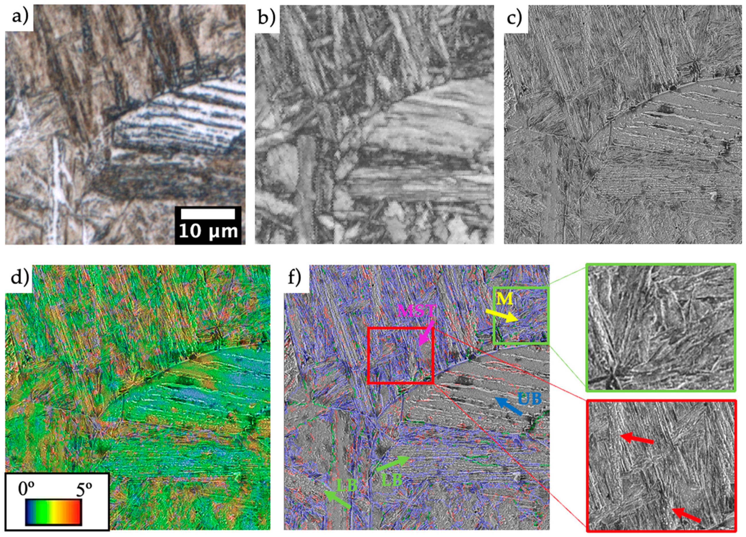
Figure 4 shows a section of a correlative data set consisting of LOM, SEM and EBSD data containing all phases to be distinguished. There, the corresponding added value of the complementary information for the identification of the occurring phases becomes clear. With the help of the high resolution of the SEM, fine carbide precipitates can be clearly identified and thus LB and MST can be reliably detected. In addition, a distinction between LB and UB is possible based on the localization and orientation of the fine carbides, which would not always be the case based purely on light microscopy images. Furthermore, contrasting artifacts as well as ambiguous morphologies can be considered with the help of the crystallographic EBSD information. Though, the most helpful information from EBSD data for identifying the different microstructural constituents is provided by the misorientation.

Used Quantification Approach: Patchwise Classification as Alternative to Semantic Segmentation

Semantic segmentation is the common DL approach for segmenting more complex problems that cannot be solved using conventional approaches, such as threshold segmentation. It is a pixelwise classification: each pixel of the image is assigned a class and thereby, the entire image is segmented [21]. Additionally, it is possible to carry out segmentation with more than two classes in the same segmentation step, which offers great added value. In order to train a model for semantic segmentation, masks must be created, in which every pixel can clearly be assigned to a specific class.
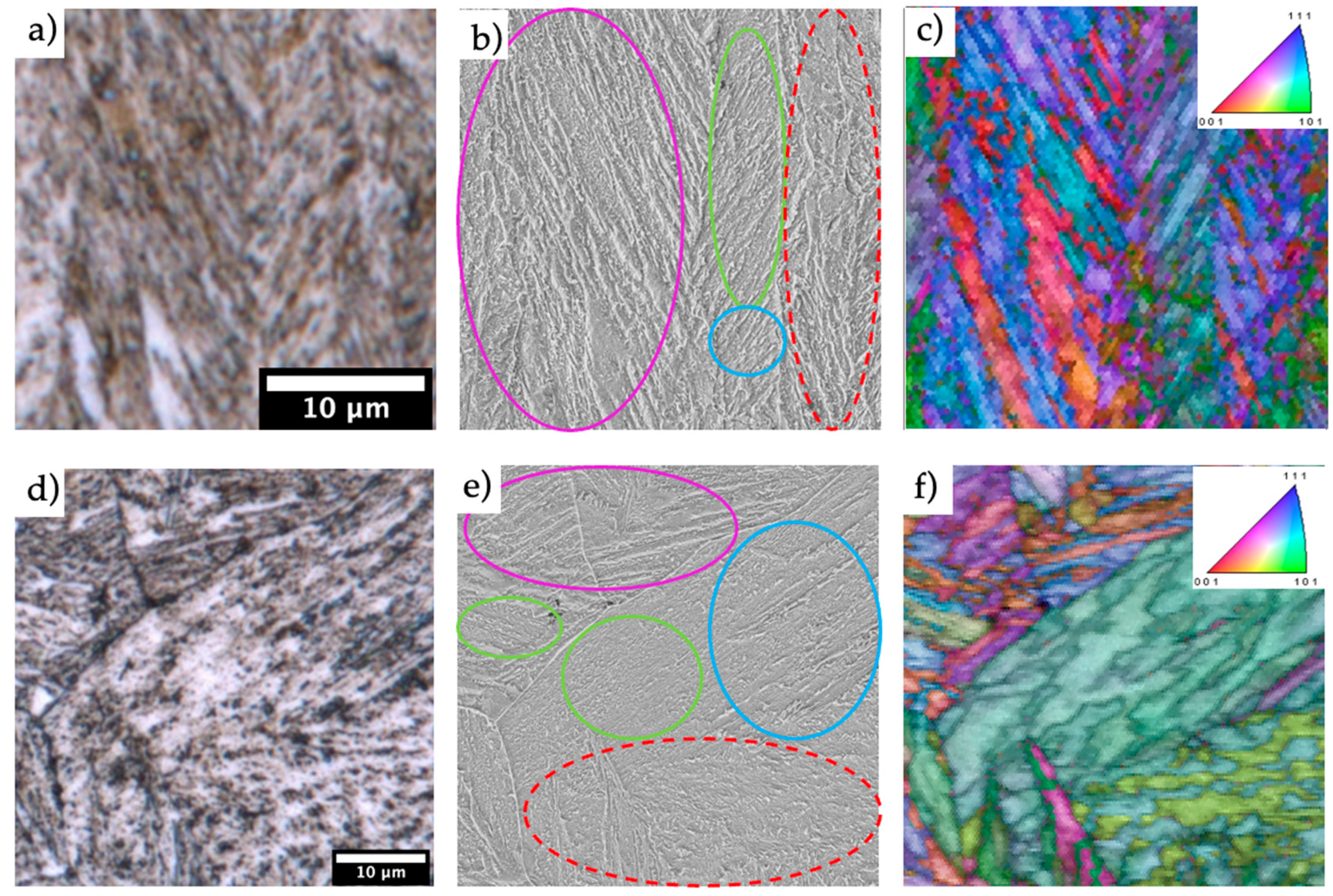
In contrast to most segmentation problems, for the microstructures of Q/QT steels it is not straightforward to create unambiguous masks to train a DL segmentation approach. In the case of dual-phase and complex phase steels, the complementary information of the correlative images is sufficient to clearly identify the respective microstructural constituents. There, the respective phases can be clearly separated from each other by grain/phase boundaries [3,6]. Morphology and corresponding misorientation information allow to confidently differentiate one phase from another. Due to the complex formation mechanisms in Q/QT steels and the resulting interwoven structure of the microstructural constituents, it is not possible to reproducibly define the boundaries of the different phase regions. In addition, various areas of the microstructure often cannot be clearly assigned to a corresponding class. Even crystallographic EBSD information, as well as corresponding high-resolution imaging techniques, often do not allow annotation with required confidence according to the common classification schemes, which is illustrated in Figure 5.
A reasonable approach would be to annotate only unambiguous regions and then assign the ambiguous regions to a common mixed class. An obvious disadvantage of this would be the great diversity of the resulting mixed class. This would accordingly mix up the characteristic visual features of the individual classes. Accordingly, it can be assumed that the significance of the decisive features for determining the clearly defined classes would decrease. Therefore, an alternative approach to segment the different microstructural constituents in Q/QT steels as reliably and unambiguously as possible was chosen in this work.
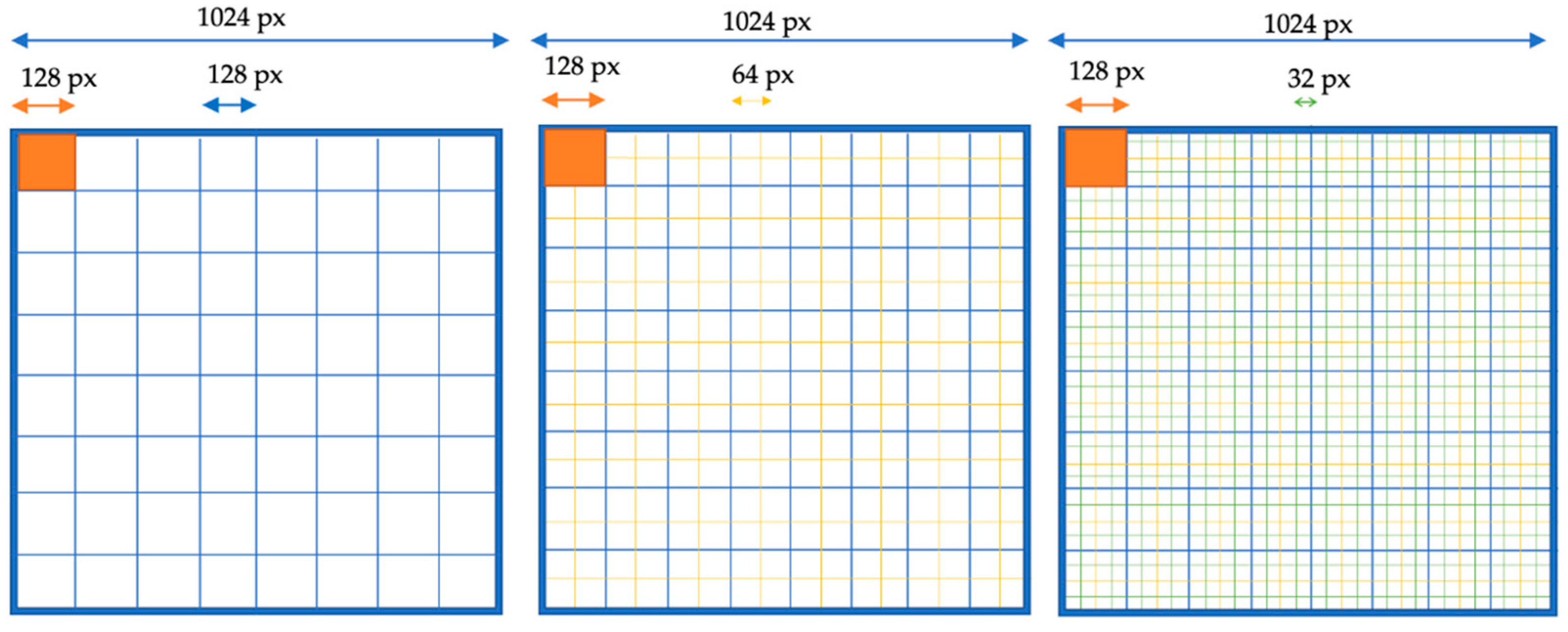
In contrast to the pixel-by-pixel approach used in semantic segmentation, this approach reduces the microstructural images to individual patches. These patches are classified individually, and the result is considered representative of the particular microstructure section. In order to be able to characterize an entire microstructure, the individual microstructural images are scanned and segmented by a CNN patch by patch using a sliding window approach [22]. Thereby, the complex problem of segmentation is reduced to a simple classification. This saves a decent amount of time during annotation, or makes annotation possible in the first place in complex cases.
The respective patch size is predefined by the CNN architecture's input size. However, in order to achieve a higher “segmentation resolution” and to better map the fine transitions between the areas of the individual microstructural components, the step size can be adjusted in the scanning process. The smaller the step size, the higher the resolution of the resulting classification map. As a result, the possible resolution of the result depends on the original resolution of the entire recording, as well as the step size with the corresponding input size and is thus, depending on the total amount of input images, limited by the computing resources.
In this approach, a classification model is trained with patches of reference states that are representative of the structural constituents that are present. With respect to the patches to be selected for training the models, only relatively unambiguous reference states are selected. Inconclusive patches are left out. The idea behind this is to classify these objectively and reproducibly by the ML model. Due to the versatility of the individual phases occurring in Q/QT steels, the training data must cover the widest possible spectrum of microstructural features and represent their high variance as accurately as possible. There is a trade-off between the amount of data and the confidence with which the data is labeled. Hence, 22 correlative data sets from the above-mentioned samples were elaborately created in the course of this work and used to extract sufficient high-quality data to build a final training dataset.
The probabilistic character of the CNN classification approach makes it possible to take the uncertainty of the ambiguous regions into account when evaluating entire microstructural images. Usually, classification CNNs give the corresponding probabilities of the available classes as output, from which a final prediction can be derived. A confidence component can be built into this approach by using appropriate thresholds with respect to the class probabilities. Thus, individual patches can be declared as uncertain with no clear class affiliation, which is an analogy to the microstructural regions that are ambiguous for experts during the characterization of the respective microstructure. This means that even ambiguous structure sections containing a combination of different phases can be identified and considered in the evaluation routine by summarizing the uncertain predictions in a separate class.

Annotations and final data set

Based on the microscopy images, a comparison of the respective structural components can be made using the morphological information after appropriate contrasting. In the case of LOM, further information is obtained by looking at the coloration. The major advantage of SEM methodology is the ability to resolve substructures, such as carbides and finer lath boundaries, which delivers essential information about the class affiliation. Considering the related step size of 0.35 µm, the resolution of the EBSD is behind those of LOM and SEM. Nevertheless, the crystallographic and misorientation information provides crucial added value in contributing to an objective labeling process.
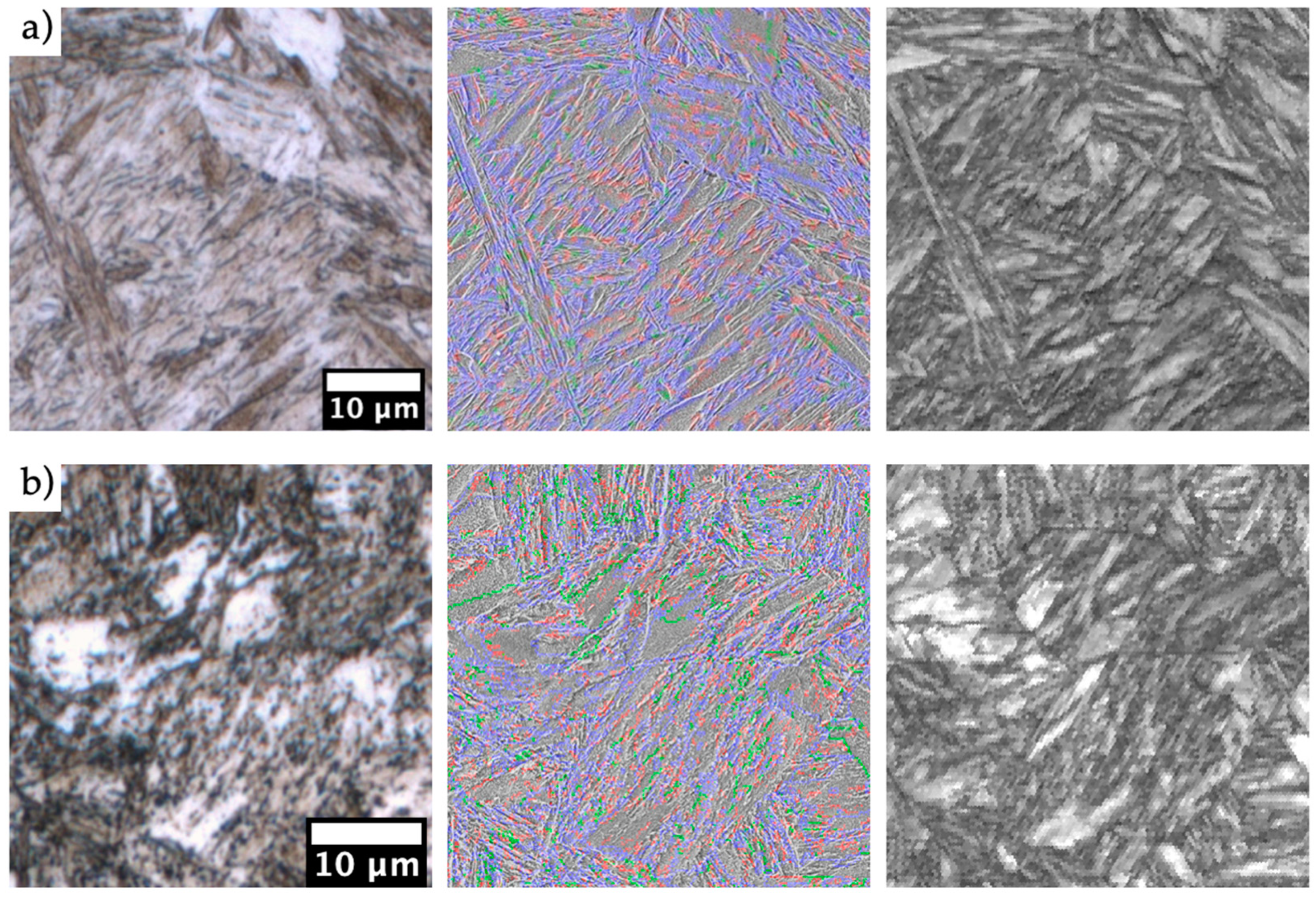
Thus, upper and lower bainite can be distinguished on the basis of the quantity and type of misorientations or boundaries that occur [14]. Upper bainite contains a higher fraction of low misorientations (<20º), as well as a low proportion of misorientations (>40º). In the case of the lower bainite, this situation is reversed. Bainitic objects also exhibit more global misorientations that create intra-structural gradients visible in the IPF. Furthermore, the packet size can provide information about a distinction between martensite and the different bainite types [23]. In addition, the IQ can be used to compare local dislocation densities qualitatively. Thus, this information can provide further evidence for an assignment to the ground truth [24,25]. Due to the displacive forming mechanism, martensite exhibits the highest misorientations, as well as the highest density of dislocations. The individual martensite plates are very well visible and separable from each other in the IPF as well as in IQ map [26]. Their lath boundaries are strongly contrasted and characterized by high misorientations (>50º). It was observed that the contrast of the lath boundaries is weaker in tempered martensite within the IQ map. In general, the contours become more blurred. The amount of high misorientations decreases slightly, whereas the amount of smaller misorientations increases during the tempering process. This is shown in Figure 7b) by the number of green interfaces. This is the same material as in Figure 7a), except that it has been subjected to a subsequent annealing process. These phenomena can be attributed to carbon diffusion during the tempering process.
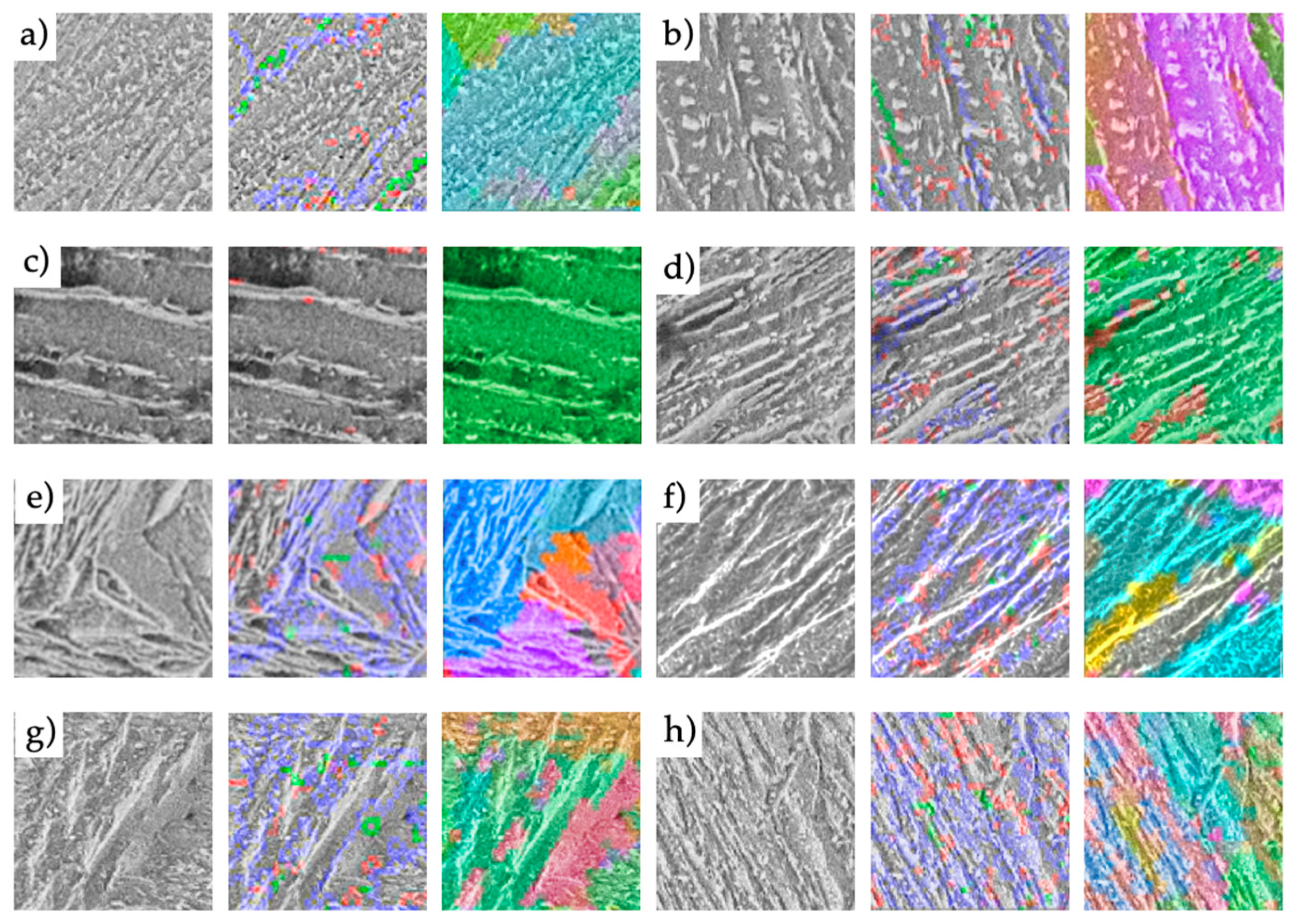
The key to this approach of quantitative structural evaluation via patch-wise classification lies in the creation of representative and well-founded data sets. A crucial parameter for the creation of the datasets is the choice of the patch size. To use the native resolutions of the microscopes to avoid resizing and thus falsification of the morphological features by interpolation, the size scales of the microstructural constituents within the specimens examined were used as a guide. As a result, it was decided to create two separate datasets, each optimized with respect to the different microscope types, LOM and SEM. To achieve the highest possible classification resolution in the evaluation routine described above, it makes sense to keep the size of the squared patches to be classified as small as possible. The size of the characteristic morphological features of the different structural components is another limiting factor. A patch should therefore be as small as possible, but it must contain enough information to be able to assign a well-founded and objective label for the ground truth. As a result, a patch size of 128px was chosen for the SEM optimized dataset, which corresponds to a size of 6.25µm. Due to the lower resolution of the LOM, a patch size of 128px was selected, which in this case corresponds to an actual length of 12.5 µm. In the labeling process of each dataset, the corresponding microscopy images of SEM, and LOM, respectively, were first inspected. Each section, which could be a candidate to be added to the training dataset, was validated with the help of the corresponding complementary information from correlative microscopy.
To extract the patches, the different representations were overlaid in an image processing program. For this purpose, LOM, SEM images, as well as the EBSD information in the form of IPF, IQ and KAM maps and, mostly, the representation of the different misorientations in the form of boundaries with the threshold values 2, 5 and 15 degrees, were used. To mark the labeled sections, a square brush tool was used to create masks of the respective four classes, respectively for the LOM and the SEM optimized dataset. These binary masks were then used to automatically extract the corresponding labeled patches from LOM and SEM images, respectively.
When creating the SEM data set, superimposed representation of the misorientations combined with the SEM images were used in order to be able to reproducible assign more of the unclear areas to one of the classes, which may have appeared ambiguous due to possible contrasting artifacts. The crucial information, e.g., regarding the orientation of the precipitated carbides, which is to be regarded as a decisive distinguishing criterion, is most evident in the SEM images themselves, as it is the highest-resolution method. Therefore, although it proved to be very time-consuming to create a well-founded data set from SEM patches due to the volume of information as well as criterions to be considered, it can be evaluated with great confidence as objective and representative.
Figure 8 shows a selection of characteristic features of the individual classes within the different complementary information sources. Thus, LB, shown in a) and b) is characterized by moderate misorientations, as well as the orientation and size of the carbides within the laths. The IPF overlay shows similar orientations of the adjacent laths. UB, as shown in c) and d) is characterized by elongated carbide precipitation between the laths, which have a homogeneous orientation by comparison, sometimes with pronounced gradients within the laths, and the least misorientation. For the remaining structural components M, shown in e) and f) and MST, shown in g) and h), the disordered orientation of the individual laths can be confirmed looking at the IPF. Here, MST can be identified by the fine and disordered carbide precipitates visible in the high-resolution SEM image.
The creation of the LOM data set proved to be much more complex. In order to be able to train a model that is able to assign the patches to a class, the input image must have sufficient characteristic visual features. For some patches that can be clearly assigned to a class based on the SEM image, a clear classification based on the LOM images was not possible. The resolution of the LOM was simply not sufficient to represent the fine microstructural features appropriately. For this reason, the corresponding input size of the LOM dataset was adjusted upward, as mentioned above, to capture more context and more global characteristics in the dataset accordingly. When selecting the LOM patches, care had to be taken to ensure that the decisive features could be identified solely based on the LOM image. The corresponding correlative information from SEM and EBSD should therefore only be consulted as additional information. Due to the increased input size, the number of possible representative areas was reduced. The reason for this is that the consideration of larger sample areas, accompanied by a larger patch size, results in fewer homogeneous areas that can be predominantly assigned to one microstructural constituent. This results, on the one hand, in a smaller amount of training data, which is not insignificant for DL applications, and, on the other hand, in patches that also include more visual features of further microstructural components in comparison to the SEM patches.
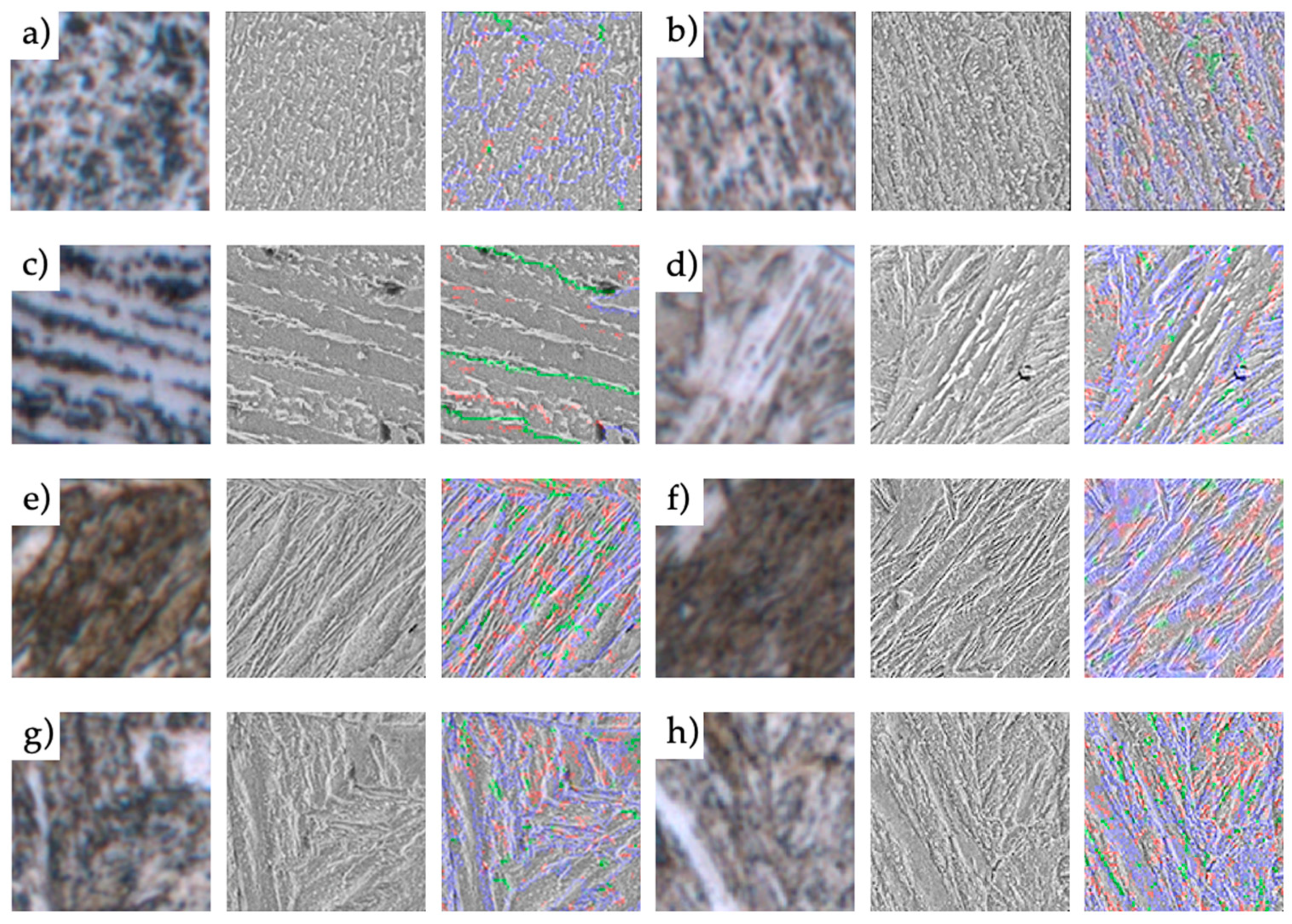
Figure 9 shows a selection of labeled patches based on the LOM dataset. Using the same characteristics outlined in case of Figure 8, the potential reference ranges were validated using the complementary information from the correlative datasets.
However, the explained compromise regarding the adjusted patch size of the LOM dataset leads to the fact that many, especially bainitic areas, are too small to fill an entire patch (Figure 8d)). As a result, features of the adjacent phases are also visible on these patches, which is unavoidable considering the amount of data required to capture the variety of the phases occurring in real Q/QT steels. Accordingly, these areas were nevertheless included in the data set. Care was taken to ensure that the characteristic areas occupy most of the patch area and are located in the center. However, this could prove to be advantageous for the evaluation routine explained, since the patches often contain more than one phase when the moving window approach is used.
Intensive review of the correlative data sets in a cross-scale and holistic approach revealed fundamental problems in assigning well-founded ground truth in the case if no complementary information was available and only the LOM images were used for the labeling processes. In the process, not only are the present micrographs accepted as such, but they are critically scrutinized along the entire process of data acquisition. Thus, additional information, such as differences in chemical composition, the manufacturing processes of the samples, as well as contrasting and methodological influences are also considered. Here, correlative microscopy enhances the interpretation of this information
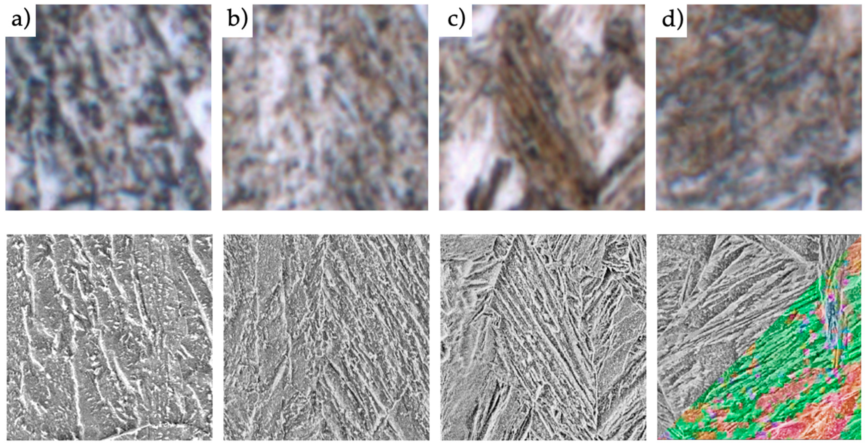
Figure 10 illustrates patches of the LOM optimized dataset with size of 12.5 µm, for which the exclusive use of LOM images for the labeling process could be quite misleading. Here, based on the visual characteristics, it can quickly lead to false labels regarding the assignment of ground truth.
Thus, a) appears to be lower bainite based on the LOM patch. This is indicated by the visible preferred orientation of the bainite plates, as well as the brownish coloration, which is caused by the finely precipitated carbides. However, if we now look at the high-resolution SEM image, it becomes apparent that the majority of the carbides has not precipitated within the laths, but that they have formed between the very fine bainitic laths. Thus, this is extremely fine upper bainite according to the common classification schemes.
Looking at the LOM micrograph of patch b), one would possibly choose martensite for classification as an experienced expert. This is supported by the disordered, lathlike morphology and the distinct coloration of the features. However, with the aid of the corresponding SEM image, the extremely fine, disordered precipitation of the cementite particles becomes clear, which in combination with the previously named morphology is a characteristic of tempered martensite.
Based on the pronounced dark brown coloration, as well as misinterpreting lath boundaries, the LOM patch shown in c) indicates a martensitic affiliation. Like a), however, the coloration can be attributed to the fineness of the cementite lamellae, which is even more pronounced in this case. Again, it can be assumed that according to the characteristics it deals with very fine upper bainite.
Due to the dark spots in combination with a light brown coloration, both corresponding to a fine dispersion of small cementite precipitations, one expects an assignment to lower bainite or tempered martensite for d). With the help of the SEM the distinct topography becomes visible, which provides a higher confidence in an assignment to the latter.
The holistic approach via correlative microscopy, which also takes into account the significant influence of contrasting as part of specimen preparation with regard to imaging, can identify further misleading factors.
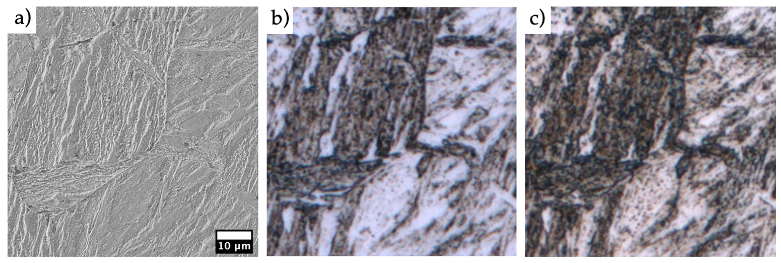
Figure 11 again illustrates the problematic reproducibility of electrochemical etching processes. After contrasting under apparently identical conditions b) and c), the correlative LOM images reveal an obvious difference. In c), especially the precipitated carbides within the microstructure, which was identified as tempered martensite, are clearly more pronounced, which simplifies an assessment as such. Based on b), one could also assume that it is martensite. Once again, only the high-resolution SEM image provides clarity regarding an unambiguous assignment.
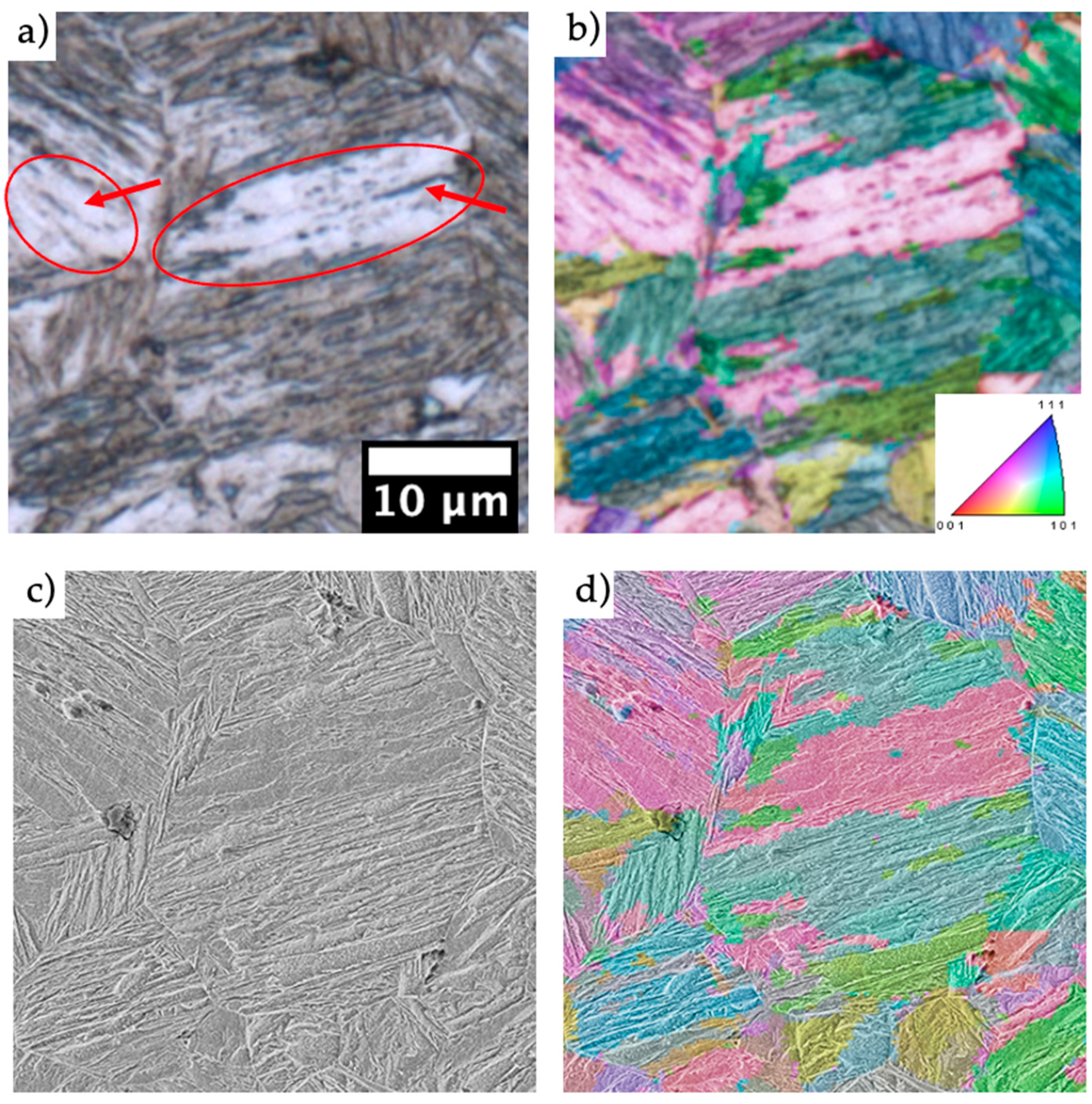
An orientation dependence of the Nital etching was observed across all specimens. Crystal orientations of <100> show a significantly reduced etching effect, as shown in Figure 12 [27]. As a result, the areas in the LOM appear bright, similar to areas associated with upper bainite. Though, the high-resolution SEM micrograph reveals the presence of martensitic topography, which due to the reduced etchability is not as pronounced as those regions with different crystal orientation. Therefore, it is not visible in the LOM image. Additionally, selective contrasting of the lath boundaries of the martensite reinforces the false impression, so that confusion with upper bainite can quickly arise (red marking).
Considering the problems demonstrated in this section, it can be concluded again that the most challenging problem behind the application of modern ML approaches in the field of materials science is finding an absolute ground truth. Considering the available complementary information, as well as the occurring misleading factors, two final datasets were created based on the 22 correlative datasets, optimized for SEM and LOM images, respectively. Unfortunately, these can only be compared indirectly due to different patch sizes and different underlying slices. In conclusion, it can be stated that despite reduction to the most homogeneous patches possible, it is not possible to guarantee the correctness of all labels. Nevertheless, a lot of time and consideration of all complementary information was used to work out the underlying ground truth. This represents, at the current state of research, the best approach to a classification in terms of the structural constituents that occur in combination with the samples investigated and taking into account the widely recognized identification criteria of the common phases occurring in modern steels. In order to train the model to a certain degree of variance and to make it as robust as possible, more critical patches were also included in the data set that partially deviate from the reference states of the respective microstructural constituents to be able to characterize real Q/QT steels as successfully as possible. Ultimately, a SEM optimized training data set of 6680 individual patches (14% LB – 41% M – 25% MST – 20% UB) as well as a LOM optimized training data set of 2246 individual patches (17% LB – 40% M – 27% MST – 15% UB) has successfully been created to train respective DL Classification models as good as possible.

Deep Learning Methodology

From DL’s perspective, this results in a multiclass classification problem with the four introduced classes. For each of the three independent models, a pre-trained CNN is used based on the principle of transfer learning [28]. This is done by taking advantage of the fact that each model is already capable of reliably recognizing important visual features and extracting corresponding low- and high-level features in order to allow an accurate classification of the respective structures. Several publications could confirm that transfer learning, using pretrained weights, even using data from different domains, is beneficial to the training process and the final model’s performance in material science [27,29,30], especially if, compared to usual DL applications, only little amount of data is accessible.
As model backbones, Xception [31], ResNet50 [32] and DenseNet201 [33] seemed to yield the best results in scope of the pre-tests. Each of the architectures was used without the respective dense layers. After the convolution layers as a feature extraction, a GlobalMaxPooling operation was implemented to reduce the features to a 1D feature vector [34], which is fed into a fully connected network. The latter consists of a dense layer with 64 neurons that is connected to a dense layer with 4 neurons, corresponding to the respective number of classes. The final prediction layer uses the SoftMax activation function to be able to interpret its entries as classification probability. To reduce the overfitting, an additional dropout layer has been added after the feature extraction part, as well as the dense layer with 64 neurons.
For both SEM and LOM dataset, 128 pixels has been selected as input size, in order to use the native resolution of the respective microscope, corresponding to the earlier mentioned sample section of 6.25µm tiles for SEM and 12.5µm tiles for LOM, respectively. As preparation step the default preprocessing function of the individual CNN architectures has been used, zero-centering each color channel with respect to the ImageNet dataset, which was used to pre-train the weights. Afterwards, each dataset has been normalized to a maximum value of 1 to be processible by the CNNs. The image labels were one-hot-encoded prior to the training process. The training dataset was divided into a training and a test-set (75%-25%). To tackle the problem of class-imbalance, class-weights according to the total number of images in respect to each class within the training dataset were included [35]. As loss function, the categorical-crossentropy was used in combination with classification accuracy as validation metric.
In terms of data-augmentation, common operations such as zoom (70 – 130%), rotations (0-360º), random contrast and brightness adjustments (0 – 10 %), as well as vertical and horizontal flip were selected. The thereby emerging empty areas are filled using the “reflect” argument.
Each model was trained for 25 epochs using the Adam optimizer at a learning rate of 0.0001 and subsequently, for 10 epochs at a learning rate of 0.00001 as fine-tuning, using the Keras API of the Tensorflow implementation [36] in Google Colab Pro with access to a NVIDIA Tesla T4 GPU.

Post-Processing: Combining Predictions of Different Models

Since different CNN architectures learn, extract and process visual features in different ways, it seems reasonable to combine the predictions of several different models. This allows for increased objectivity, as well as a higher robustness. For this work three independent optimized models were trained with the same data sets. In scope of a combined evaluation, each of these models independently classify the individual patches of the microstructure image to be analyzed. The corresponding predictions then contribute accordingly to the final classification. These are summarized and equally influence the final prediction within the framework of the majority voting approach used.
In the majority voting approach, the final prediction emerges based on the majority occurrence of the predictions after consideration of the respective threshold value. Accordingly, the final prediction must correspond to at least two of the three predictions resulting from the models used. In case either three different predictions are made by the separate models, or in case the majority of the predictions are to be assigned to the additional class of uncertainty after filtering by the confidence threshold, this will thus be the prognosis as final prediction.
A subsequent median filter with a kernel size corresponding to the corresponding step size leads to a removal of undesired artifacts, as well as a smoothing of the boundaries of the respective phase regions.

3. Results and Discussion

Classification Model Results

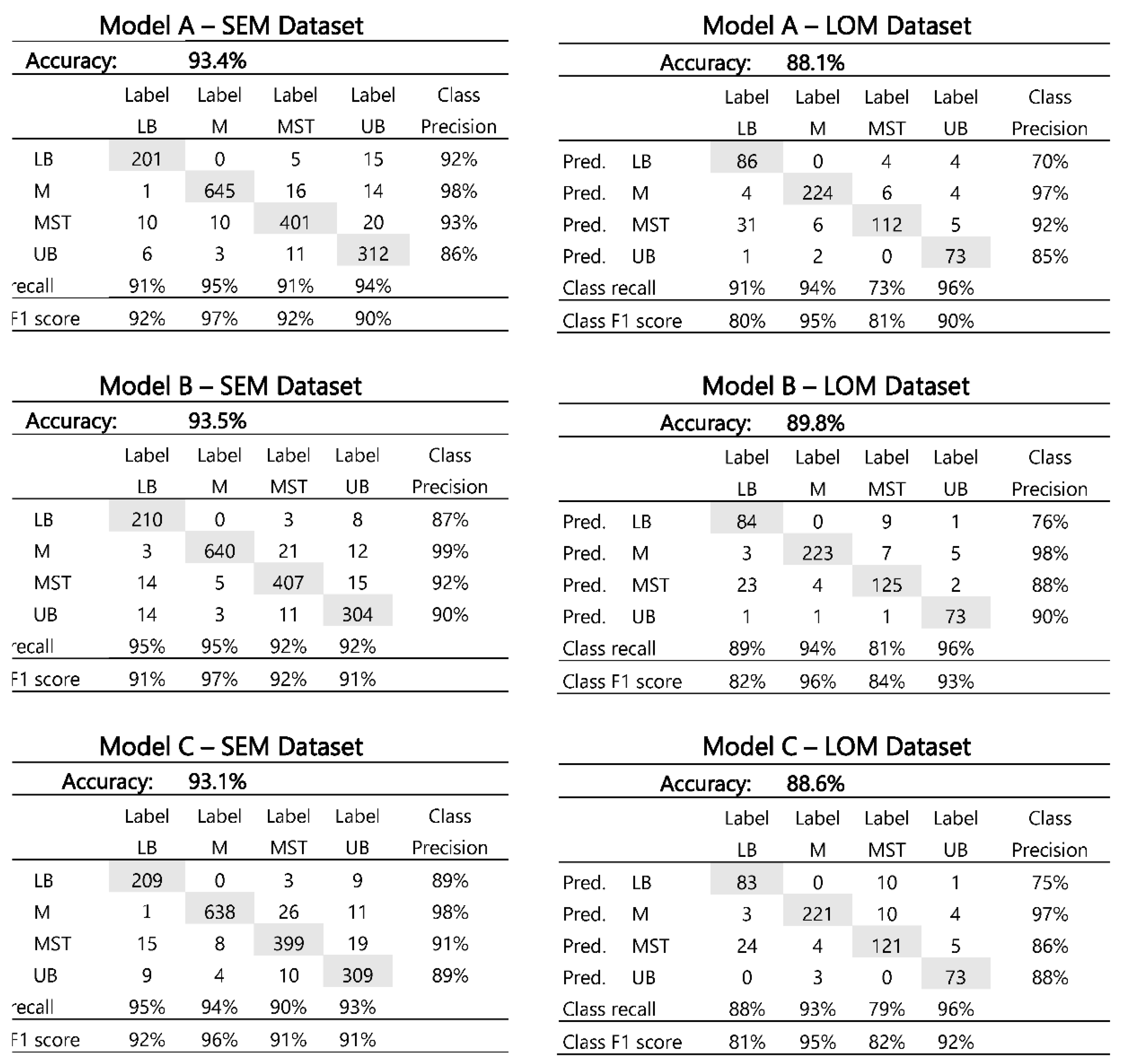
After training the respective architectures with each dataset, LOM, and SEM, the following performance could be achieved on the unseen test sets. As mentioned in the methodology part, model A is based on Xception, model B uses a DenseNet backbone, whereas model C consists of a ResNet.
Table 1. Summary of the confidence matrix combined with respective metrics, such as precision, recall and F1 score and overall accuracy of the three different architectures (Model A, B & C) for being trained on the SEM and LOM datasets.
Preprints 78969 i001
Overall, the three models could achieve an average accuracy of 88.8% for the LOM and 93.7% for the SEM dataset, respectively. These are exceptional results considering the high complexity due to the fine differences between the microstructural patches. With the standard deviation of 0.7% between the different architectures, and 0.6% in case of the SEM dataset, the performance between the models is quite homogeneous on both datasets.
Using the SEM patches delivers significantly higher performances. For example, the mean precision in classification of martensite reached a value of 98.3%. Thus, martensite was most reliably identified as such among all the classes, due to its distinct morphology which differs more from the other classes. Surprisingly, in the SEM dataset, the objects belonging to the UB class achieved the lowest relative accuracy. In the LOM dataset, however, the UB patches were the second best identified as such.
There, the martensite class also achieves the highest precision. Thus, in the case of the SEM images, each model was able to detect the subtle differences between LB and MST. From this it can be concluded that the models in relation to SEM images are successfully able to identify and process the differences in topography, as well as the fine discrimination criteria regarding the precipitation of the carbides in microscopic images of Q/QT steels. Once again, the extraordinary ability of modern DL approaches to independently learn decisive criteria based on visual features and to apply them in a reproducible manner became evident.
When looking at the LOM data, however, the comparatively low precision of averaged 73.7% in the classification of the LB class is noticeable. This also reflects the problems and resulting concerns during the annotation process of the LOM images. Based purely on LOM images, it was often not possible to distinguish LB from MST, so that the corresponding SEM images had to be consulted. Representing this fact, most of the misclassified patches of the LB class are assigned to the class of the MST.
Despite the remarkable classification accuracies, it is of great importance to investigate the models' misclassifications in detail. Only in this way can the possibilities and limits of the models really be assessed. When considering the misclassified patches of the SEM dataset, it must be admitted that almost none of the misclassified excerpts can undoubtedly be assigned to the corresponding label. Often, these examples were assigned to the respective ground truth class on the basis of complementary information and a more global view, with the aim of being able to represent as much variance as possible. Most of them leave some room for interpretation and a residual degree of subjectivity.
Patch a) shown in Figure 13 was incorrectly classified as UB from two of the three models. It clearly shows oriented lath-like structures with slightly pronounced carbides along the axis (red arrows). Due to the majority of particles being precipitated within the laths it was labeled as LB (black arrows). However, this lack of clarity is expressed in a low prediction probability of less than 60% for each model. The counterpart to this is provided by b). Here, due to the fact that the majority of the carbides run coherently along the laths, a classification to class UB was chosen (black arrows). Nevertheless, carbide precipitates also occur occasionally within the laths (red arrows), which would confirm the prediction of the model. In contrast to the first two examples, patch c) was assigned to the wrong class with high confidence (>90% probability). Due to the pronounced parallel and comparatively homogeneous edges throughout the patch, these boundaries of the martensitic laths were misinterpreted as those of the UB (red arrows). However, additional global information (e.g., larger range for a given input size) could lead to a correction by the model by identifying it at martensite.
In MST patch d), which was labeled as such based-on topography, the significance of the aligned laths in combination with the carbides precipitated within them (black arrows) apparently predominated, so the model classified this as LB.
In summary, using the SEM dataset, no misclassified patches could be identified for which the model’s prediction could be considered as totally inconclusive. Thus, no decisive argument can be found to question the general validity and reliability of the models in view of a given similarity to the specimens being considered within this study at this point.
For the LOM dataset, the number of correctly classified patches in the LB, M, and UB classes differs only marginally. Here, the greatest difference between the different architectures is expressed in the MST class. For the majority of the overall misclassified patches, the insufficient resolution of the LOM was found to be the cause. For the corresponding patches, the respective ground truth was selected based on the underlying complementary information. Minimal misinterpretations already lead to incorrect decisions by the model, which are, however, very comprehensible on closer examination.
For the classification of the LOM images, patch a) from Figure 14 was predicted as UB and LB, whereas it was labeled as MST. These decisions are both understandable due to the slightly brownish coloration in combination with the precipitated carbides, as well as due to possible contrasting lath boundaries of the avoidable bainite. However, due to the needle-like topography, which is only enhanced on the SEM image, the decision was made in favor of MST during the labeling process. Though, since all three models predicted different classes, the interpretability will be represented as an unclear label in the following post-processing routine during the quantification of an entire microstructural image.
A similar case occurs in patch b). Here, the as M incorrectly classified patch c) with ground truth UB represents the problem that already has been shown in Figure 10c) in an even more difficult way. There, the bainitic laths are extremely fine which allows misinterpretation towards the martensitic class. Additionally, in contrast to the previous example from Figure 10c), the bainitic features do not fill the entire patch, but are additionally surrounded by martensitic regions. Hence, this was one of the most ambiguous examples within the test dataset.
In patch d) an inverse misclassification compared to c) can be seen. There, the white shimmering areas between the sufficiently contrasted lath boundaries on the upper center, as well as the white region on the lower right, lead through the otherwise brownish coloration of the microstructure to a falsified impression. Through looking at the IPF, the assignment of those areas to the <100> orientation can be found. Thus, the orientation contrast observed during the labeling process is also involved in a misjudgment of the CNN. However, the fine and disordered needle structure of the martensite plates can be identified by SEM, which is why this class was chosen in the labeling process.
In summary, the classification of LOM patches performed much better than expected at the beginning. Compared to the SEM images, the biggest bottleneck of using the LOM images is the resolution, which is accompanied by a lack of crucial detailed information. Nevertheless, very high accuracies were achieved and the wrong decisions of the CNN could be comprehended in most cases, and most likely, would be confirmed by human experts in a similar manner.
All in all, based on the results presented here, it can be concluded that the trained models are very well able to perform a good differentiation between the individual classes based on both LOM and SEM images. The surprisingly high accuracies, despite the underlying complexity, illustrate the adaptability of the modern DL approaches. Despite the inevitable room for interpretation in a classification based on the given classification schemes and the residual subjectivity that is unavoidable in these approaches to microstructure evaluation, the classification approaches have the ability to successfully recognize and process the fine discriminatory criteria. It can be assumed that the performance of the models trained here is very close to that of an experienced expert, given the richness of the complementary information used to find an objective ground truth and its overwhelming ability to apply this knowledge. Nevertheless, this knowledge is limited to exactly these types of Q/QT steels with which the model was trained. The great added value here, however, is the existing reproducibility compared to conventional expert opinions.

Patch-wise Classification using a Sliding Window Technique as Segmentation Approach

In the following section, the trained models are used to quantify entire microstructural images. The sliding window approach used for this purpose allows segmentation using classification models that need a fixed patch size of 128px, respectively, as an input.
Here, the results of LOM recordings and SEM images are compared with each other, and the similarities and differences are discussed. Thereby the aim is to clarify to what extent a quantification based on the LOM images is sufficient as the simplest and fastest method, and to what extent more complex high-resolution SEM images are needed for a representative evaluation.
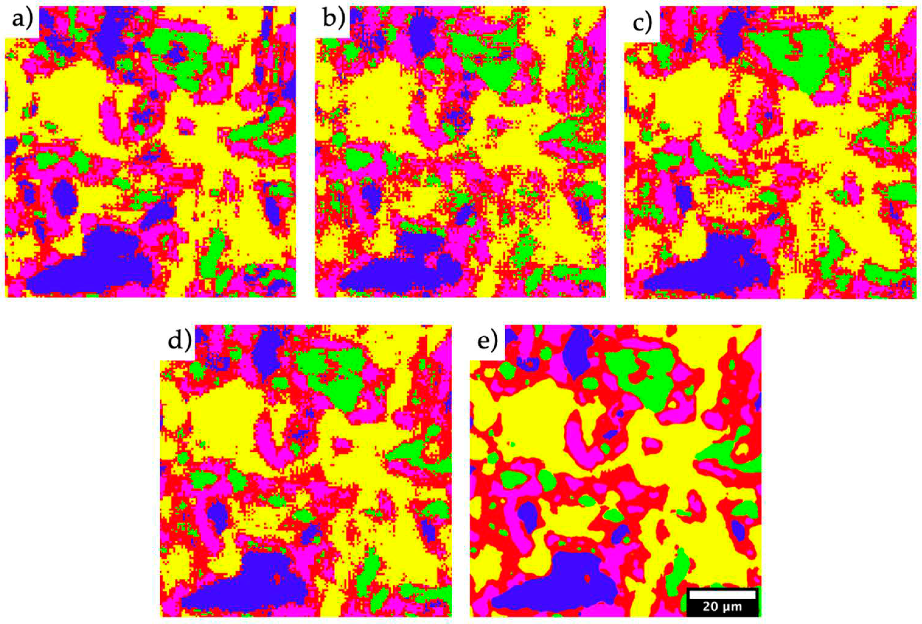
In Figure 15a-c, the different segmentation results of the trained models can be examined separately. It is noticeable that the majority of the color-coded predictions (LB – green, M – yellow, MST – purple, UB – blue, uncertain – red) are very comparable between the individual models. Nevertheless, there are isolated areas in which the different models also produce different estimates. As described in the methodology section, the final decision is made by majority vote. This allows an increase in objectivity and a reduction of errors, similar to a consultation between experts.
In order to eliminate individual artifacts and to smooth the boundaries of the detected phase ranges, a median filter with a kernel size corresponding to the respective step size is used as the final step of post processing.
Consequently, an evaluation on the majority vote requires a classification by each of the models used and then a unification of the predictions. The quantification of a 200x200 µm test area with a high-resolution SEM image with a step size of 16 px (approx. 0.8 µm) required 3 minutes in the Colab environment used for this purpose. The duration is thus dependent on the dimension of the section to be quantified, as well as the step size, which corresponds to the resolution of the evaluation, and can thus be adjusted accordingly.
The confidence threshold for decision-making in this case was deliberately chosen to be extremely high at 75%. This is usually the majority, i.e., 50%. In this case, however, this illustrates the problems discussed in the segmentation of complex Q/QT steels. Similar to the labeling process by experts, the transition zones between two phase areas have been classified as ambiguous (red). This was the basic idea behind the patch-wise approach: to be able to precisely map this uncertainty, without having to add a separate class within the training data, which then contains characteristic visual features of various other classes.
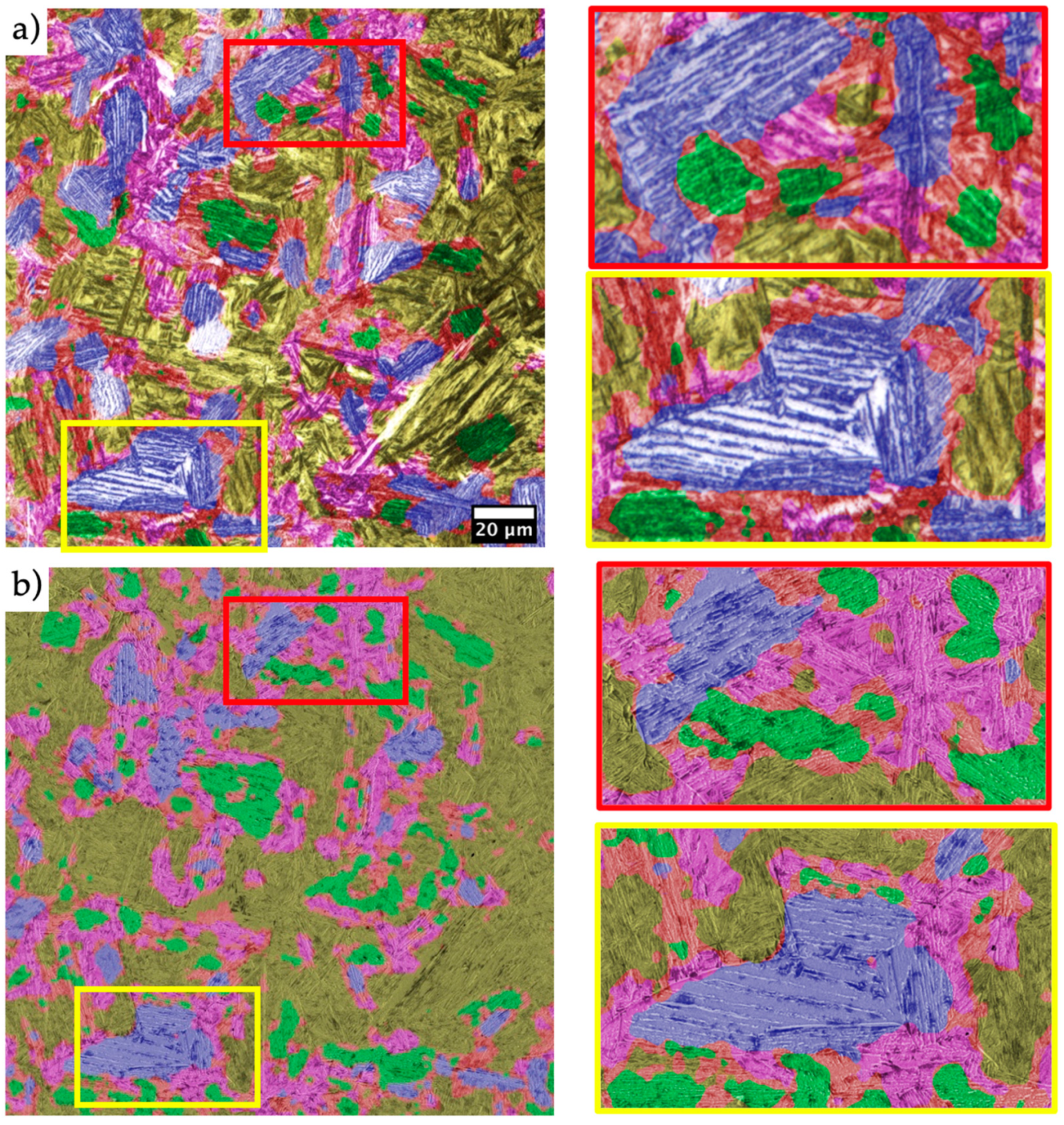
At first glance, a large part of the segmented areas between LOM and SEM image matches. The discrepancies become clearer in the enlarged section (red). There, the UB fraction (blue) in the LOM is overestimated. This is due to the strong expression of the laths in the LOM. A closer look in the SEM confirms the prediction of the model based on the SEM data regarding a classification in favor of the MST class. Furthermore, there are occasional confusions between UB (blue) and LB (green) within the LOM. As explained in the section above, this is due to the insufficient resolution of the precipitated carbides between and within the ferritic laths and thus again represents the greatest limitation of an evaluation based on LOM as a simpler methodology.
It would be desirable to reduce the proportion of misclassifications and to increase the lack of unambiguity by an increased uncertainty, expressed by a larger proportion of the corresponding uncertain class. This can be achieved by adjusting the confidence threshold upward. Thus, in general, the proportion of the additional class representing the model uncertainty can be interpreted as a measure of the complexity of the analyzed microstructure.
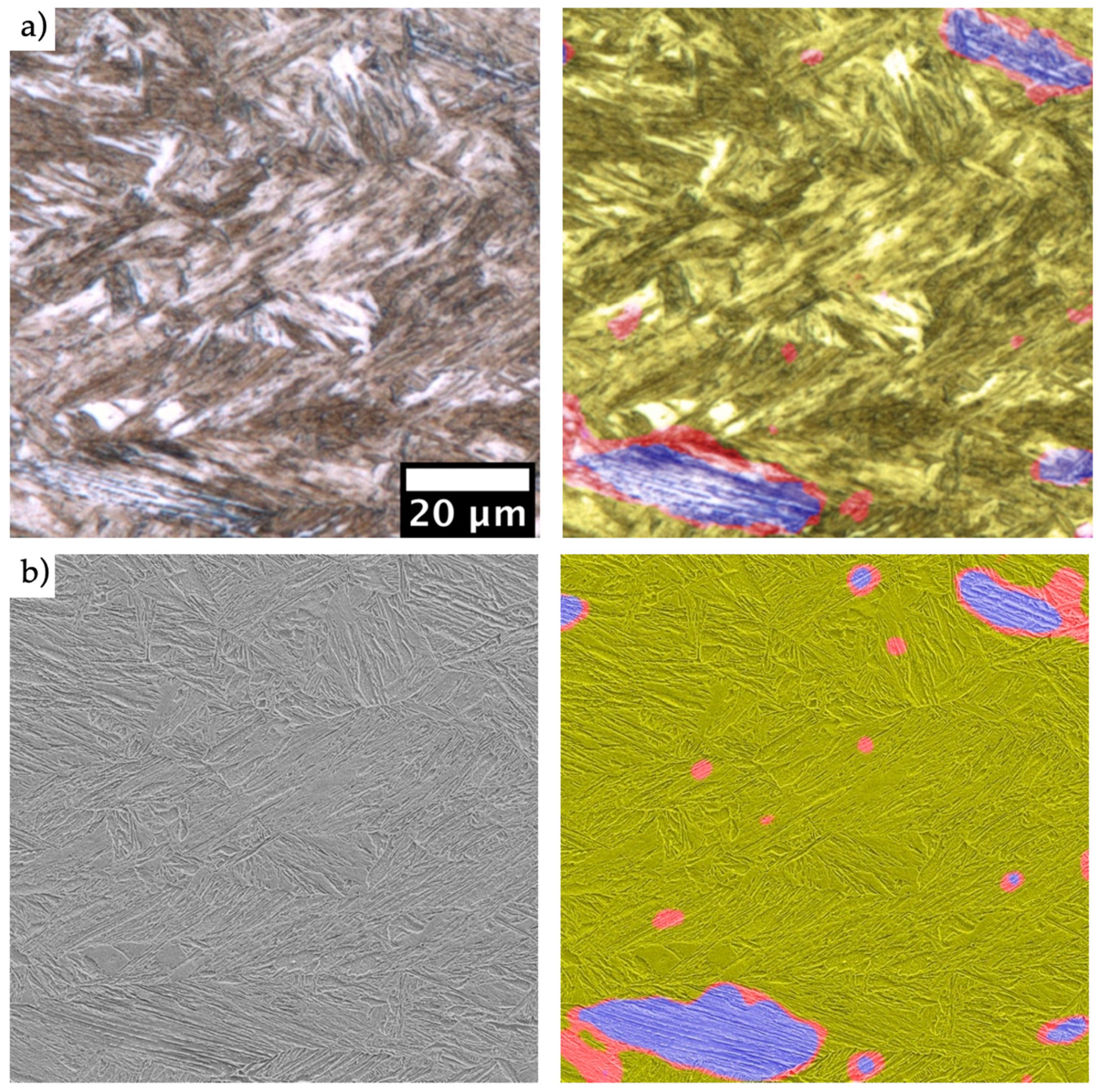
This martensitic (yellow) steel with areas of upper bainite (blue) illustrates the robustness of the underlying models (see Figure 17). The quantification based on the LOM image corresponds, apart from minimal differences, to that of the SEM image. Thus, it can be concluded that there are applications in which the evaluation based on the easier to generate LOM image is undoubtedly sufficient for a reliable characterization. Although the corresponding UB areas are relatively small and the differences of the visual features of the UB in this case to that of the M are only minor, the model was able to identify all corresponding areas from the LOM image.
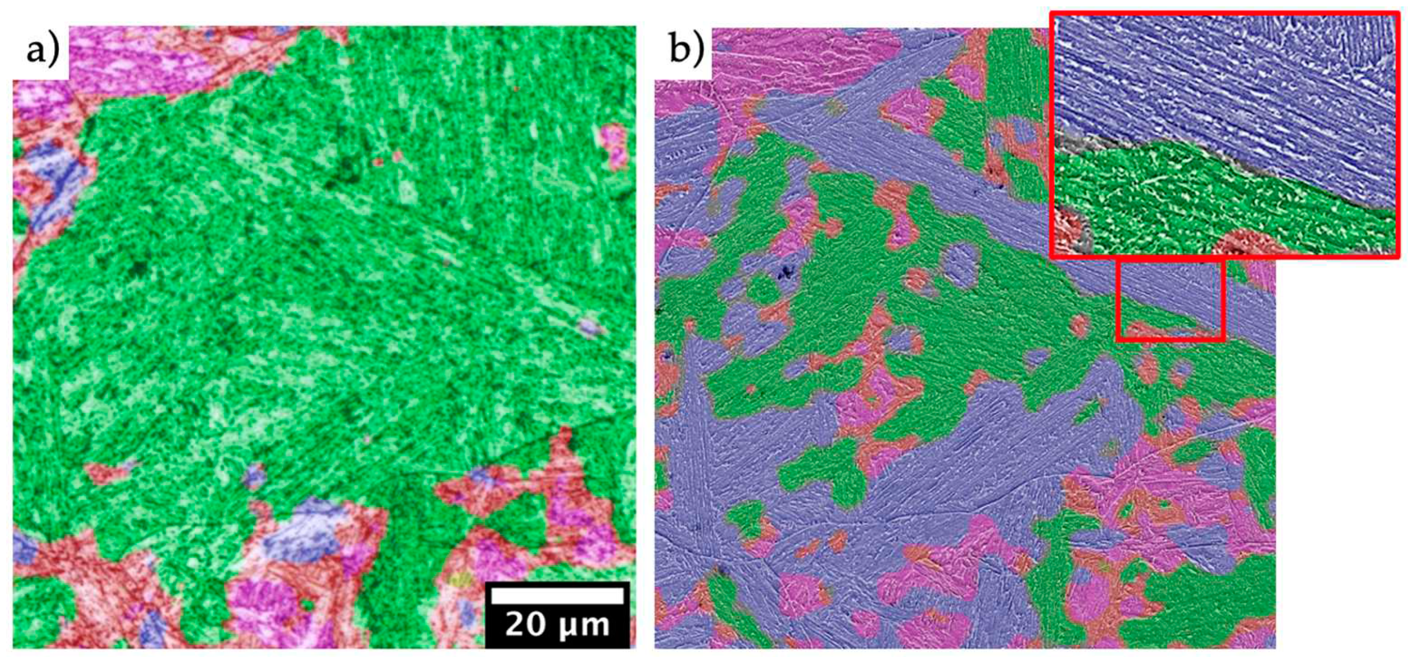
In contrast, Figure 18 again illustrates the limitations of evaluating only LOM images. Based on the LOM image, most of this section is assigned to the LB phase. Based on the SEM image, the majority can be assigned to the UB phase. Both decisions are comprehensible based on the respective images. However, only the SEM image reveals the specific morphology of the precipitated carbides. Although these are also finely distributed and not excessively coherent, a closer look reveals that they were precipitated between the extremely fine laths along their boundaries, which confirms the assessment as UB. Thus, it can be concluded once again that the evaluation of both recording methods can also be carried out on unseen steels, but that the significance of the LOM recording depends on the complexity and fineness of the present structure. If the characteristic features are too fine, it is not possible to evaluate the LOM recording alone to yield the desired result. Nevertheless, even in the LOM, the isolated areas belonging to the MST class (purple) could be correctly identified, which reduces the aforementioned concerns about limited distinguishability between LB and MST. In this case, the topography of the MST is sufficiently contrasted that it can be reliably distinguished from the LB based on the LOM micrograph.
In summary, the functionality and applicability of the proposed approach could be demonstrated. The relatively high variance within the elaborate datasets, consisting of 22 samples, allowed to train a robust model that allows a successful application of the learned criteria and characteristic visual features. Thus, LOM and SEM microstructural images that included the diverse microstructural constituents were successfully segmented and quantified. An example was used to show the extent to which it is sufficient to carry out quantification using the simpler LOM methodology and where its limitations are. Thus, high-resolution SEM images are necessary for a meaningful evaluation of the fine and more complex microstructural constituents. However, this also applies to a conventional evaluation by a metallographer. The great added value in the automation of this evaluation routine by the DL approach presented here therefore also lies in the reproducibility. Assuming reproducible contrasting and constant recording conditions for comparable steels, the quantifications by this approach are preferable to the subjective evaluations by different experts. In order to further improve the robustness and reliability of this approach, it is recommended to generate additional well-founded training data, which may additionally represent an even higher variance with respect to chemical composition, process conditions, as well as acquisition conditions including more variable contrasting methods.

4. Conclusions

Quenched as well as quenched and tempered steels are known for their wide range of applications and high complexity of microstructures which can often mainly qualitatively assessed using higher-resolution microscopy methods due to their fine microstructural features. For the segmentation of these type of steel microstructures, an automated, objective, and reproducible machine learning (ML) approach is proposed. The four microstructural constituents martensite, tempered martensite, lower bainite and upper bainite are considered for the segmentation, which can all be present simultaneously in a single region of interest. Instead of the typical semantic segmentation, a patch-wise classification is used, which significantly simplifies the annotations required for the ML approach. An advanced sliding window approach combined with suitable post-processing nevertheless enables a finely resolved segmentation based on the classifications.
The foundation for a successful implementation is a correlative microscopy approach, combining light optical microscope (LOM), scanning electron microscope (SEM) and electron backscatter diffraction (EBSD). Additional information from EBSD was essential for a well-funded and objective assignment of the ground truth. From this correlative characterization, datasets with a large microstructural diversity were generated for a LOM and a SEM classification aiming to evaluate limits of the proposed model’s robustness.
The ML models achieved an accuracy of 88.8% for the LOM patches and 93.7% for the SEM patches. Building on this, the segmentation of new unseen images was demonstrated. The possibilities and limitations of segmentation, also with regard to potential uncertainties in the assignment of the ground truth, were discussed in detail. In addition, the authors specifically investigated which performance is still achievable using only low-resolution LOM images, and for which use cases higher resolution SEM images are preferable. The presented approach offers a universally valid alternative to a quantitative evaluation of highly-complex microstructures, where an unambiguous generation of pixel-wise training masks, is not possible in a reproducible way, similar to this showcase of Q/QT steels. This ML-based quantification is noted for its automation, objectivity, and reproducibility, and enables microstructural analyses of previously unfeasible quality and detail and thus, can form the basis for future process–microstructure–property correlations as well as for improving industrial quality control.

Author Contributions

Conceptualization, B.-I. B., M.M. and D.B.; methodology, B.-I. B., M.M.; software, B.-I. B.; validation, B.-I. B., M.M.; formal analysis, B.-I. B., M.M. ; investigation, B.-I. B.; resources, B.-I. B.; data curation, B.-I. B.; writing—original draft preparation, B.-I. B., M.M.; writing—review and editing, B.-I. B., M.M., D.B. and T.S.; visualization, B.-I. B.; supervision, F.M., D.B.; project administration, T.S., D.B. and F.M; funding acquisition, M.M., D.B., F.M and T.S. All authors have read and agreed to the published version of the manuscript.

Funding

This research was funded by the EFRE Funds of the European Commission.

Data Availability Statement

The dataset presented in this article are not readily available yet because it is still part of an ongoing study. Requests to access the datasets should be directed to bjoernivo.bachmann@uni-saarland.de.

Acknowledgments

The authors thank steel manufacturer Aktien-Gesellschaft der Dillinger Hüttenwerke for the strategic collaboration in which this research project was elaborated, and for providing the sample material. The EFRE Funds of the European Commission and the State Chancellery of Saarland for support of activities within the ZuMat project is acknowledged. We acknowledge support by the Deutsche Forschungsgemeinschaft (DFG, German Research Foundation).

Conflicts of Interest

TS was employed by the company Aktien-Gesellschaft der Dillinger Hüttenwerke. The remaining authors declare that the research was conducted in the absence of any commercial or financial relationships that could be construed as a potential conflict of interest.

References

  1. Stuckner, J.; Harder, B.; Smith, T.M. Microstructure Segmentation With Deep Learning Encoders Pre-Trained on a Large Microscopy Dataset. 2022. Available online: http://www.sti.nasa.gov (accessed on 8 August 2022).
  2. Decost, B.L.; Holm, E.A. A computer vision approach for automated analysis and classification of microstructural image data. Comput Mater Sci 2015, 110, 126–133. [Google Scholar] [CrossRef]
  3. Azimi, S.M.; Britz, D.; Engstler, M.; Fritz, M.; Mücklich, F. Advanced steel microstructural classification by deep learning methods. Sci Rep 2018, 8, 1–14. [Google Scholar] [CrossRef] [PubMed]
  4. Müller, M.; Britz, D.; Ulrich, L.; Staudt, T.; Mücklich, F. Classification of bainitic structures using textural parameters and machine learning techniques. Metals 2020, 10, 630. [Google Scholar] [CrossRef]
  5. Ronneberger, O.; Fischer, P.; Brox, T. U-Net: Convolutional Networks for Biomedical Image Segmentation. Lecture Notes in Computer Science (including subseries Lecture Notes in Artificial Intelligence and Lecture Notes in Bioinformatics) 2015, 9351, 234–241. [Google Scholar] [CrossRef]
  6. Durmaz, A.R.; et al. A deep learning approach for complex microstructure inference. Nat Commun 2021, 12, 1–15. [Google Scholar] [CrossRef] [PubMed]
  7. Tsutsui, K.; et al. A methodology of steel microstructure recognition using SEM images by machine learning based on textural analysis. Mater Today Commun 2020, 25. [Google Scholar] [CrossRef]
  8. Zhu, B.; Chen, Z.; Hu, F.; Dai, X.; Wang, L.; Zhang, Y. Feature Extraction and Microstructural Classification of Hot Stamping Ultra-High Strength Steel by Machine Learning. JOM 74, Springer. 2022; 3466–3477. [Google Scholar] [CrossRef]
  9. Bachmann, B.I.; et al. Efficient reconstruction of prior austenite grains in steel from etched light optical micrographs using deep learning and annotations from correlative microscopy. Front Mater 2022, 9. [Google Scholar] [CrossRef]
  10. Bargel, H.-J.; Schulze, G.; Werkstoffkunde; Heidelberg, S.-V.B., 2005.
  11. Xie, B.S.; Cai, Q.W.; Yun, Y.; Li, G.S.; Ning, Z. Development of high strength ultra-heavy plate processed with gradient temperature rolling, intercritical quenching and tempering. Mater. Sci. Eng. A 2017, 680, 454–468. [Google Scholar] [CrossRef]
  12. Bhadeshia, H.D.K.H.; Honeycombe, R.; Steels: Microstructure; properties; th ed. Butterworth-Heinemann, 2017.
  13. Abe, F. Precipitate design for creep strengthening of 9% Cr tempered martensitic steel for ultra-supercritical power plants. Sci. Technol. Adv. Mater. 2008. [Google Scholar] [CrossRef]
  14. Zajac, S.; Schwinn, V.; Tacke, K.H. Characterisation and Quantification of Complex Bainitic Microstructures in High and Ultra-High Strength Linepipe Steels. Mater. Sci. Forum 500 2005, 501, 387–394. [Google Scholar] [CrossRef]
  15. Schwinn, V.; Streißelberger, A. Die Grobblechherstellung aus verfahrenstechnischer Sicht. Grobblech–Herstellung und Anwendung. Dokumentation 570, 7–16.
  16. Britz, D.; Hegetschweiler, A.; Roberts, M.; Mücklich, F. Reproducible Surface Contrasting and Orientation Correlation of Low-Carbon Steels by Time-Resolved Beraha Color Etching. Mater Perform Charact 2016, 5, 20160067. [Google Scholar] [CrossRef]
  17. Ulyanov, P.G.; et al. Microscopy of carbon steels: Combined AFM and EBSD study. Appl Surf Sci 2013, 267, 216–218. [Google Scholar] [CrossRef]
  18. “Image_Processing_with_ImageJ”.
  19. Arganda-Carreras, I.; Sorzano, C.O.S.; Marabini, R.; Carazo, J.M.; Ortiz-De-Solorzano, C.; Kybic, J. Consistent and elastic registration of histological sections using vector-spline regularization. in Lecture Notes in Computer Science (including subseries Lecture Notes in Artificial Intelligence and Lecture Notes in Bioinformatics), Springer Verlag, 2006, pp. 85–95. [CrossRef]
  20. Müller, M.; Britz, D.; Mücklich, F. Scale-bridging Microstructural Analysis – A Correlative Approach to Microstructure Quantification Combining Microscopic Images and EBSD Data. Pract. Metallogr. 2021, 58, 408–426. [Google Scholar] [CrossRef]
  21. Garcia-Garcia, A.; Orts-Escolano, S.; Oprea, S.; Villena-Martinez, V.; Garcia-Rodriguez, J. A Review on Deep Learning Techniques Applied to Semantic Segmentation. Apr. 2017, [Online]. Available online: http://arxiv.org/abs/1704.06857.
  22. Vigueras-Guillén, J.P.; et al. Fully convolutional architecture vs sliding-window CNN for corneal endothelium cell segmentation. BMC Biomed Eng 2019, 1. [Google Scholar] [CrossRef] [PubMed]
  23. Morito, S.; Pham, A.H.; Hayashi, T.; Ohba, T. Block boundary analyses to identify martensite and bainite. Mater Today Proc 2015, 2, S913–S916. [Google Scholar] [CrossRef]
  24. Pinard, P.T.; Schwedt, A.; Ramazani, A.; Prahl, U.; Richter, S. Characterization of dual-phase steel microstructure by combined submicrometer EBSD and EPMA carbon measurements. Microsc. Microanal. 2013, 996–1006. [Google Scholar] [CrossRef]
  25. Na, S.-H.; Seol, J.-B.; Jafari, M.; Park, C.-G. A correlative approach for identifying complex phases by electron backscatter diffraction and transmission electron microscopy. Appl Microsc 2017, 47, 43–49. [Google Scholar] [CrossRef]
  26. Baek, M.S.; Kim, K.S.; Park, T.W.; Ham, J.; Lee, K.A. Quantitative phase analysis of martensite-bainite steel using EBSD and its microstructure, tensile and high-cycle fatigue behaviors. Mater. Sci. Eng. A 2020, 785. [Google Scholar] [CrossRef]
  27. Ulyanov, P.G.; et al. Microscopy of carbon steels: Combined AFM and EBSD study. Appl Surf Sci 2013, 267, 216–218. [Google Scholar] [CrossRef]
  28. Tammina, S. Transfer learning using VGG-16 with Deep Convolutional Neural Network for Classifying Images. Int. J. Sci. Res. Publ. (IJSRP) 2019, 9, p9420. [Google Scholar] [CrossRef]
  29. Ajmi, C.; Zapata, J.; Elferchichi, S.; Zaafouri, A.; Laabidi, K. Deep Learning Technology for Weld Defects Classification Based on Transfer Learning and Activation Features. Adv. Mater. Sci. Eng. 2020, 2020. [Google Scholar] [CrossRef]
  30. Goetz, A.; et al. Addressing materials’ microstructure diversity using transfer learning. NPJ Comput Mater 2022, 8, 1–13. [Google Scholar] [CrossRef]
  31. Chollet, F. Xception: Deep Learning with Depthwise Separable Convolutions. October 2016, Available online: http://arxiv.org/abs/1610.02357.
  32. He, K.; Zhang, X.; Ren, S.; Sun, J. Deep Residual Learning for Image Recognition. December 2015, [Available online: http://arxiv.org/abs/1512.03385.
  33. Huang, G.; Liu, Z.; van der Maaten, L.; Weinberger, K.Q. Densely Connected Convolutional Networks. August 2016, Available online: http://arxiv.org/abs/1608.06993.
  34. Lin, M.; Chen, Q.; Yan, S. Network In Network. December 2013, Available online: http://arxiv.org/abs/1312.4400.
  35. Gour, N.; Khanna, P. Ocular diseases classification using a lightweight CNN and class weight balancing on OCT images. Multimed Tools Appl 2022, 81, 41765–41780. [Google Scholar] [CrossRef]
  36. Abadi, M. et al. TensorFlow: A System for Large-Scale Machine Learning. In 12th USENIX Symposium on Operating Systems Design and Implementation (OSDI 16); USENIX Association: Savannah, GA, USA, 2016; pp. 265–283. [Google Scholar]
Figure 2. Representative micrographs from LOM (upper row) and corresponding SEM images (lower row) showing the described microstructural constituents: a) – martensite, b) - tempered martensite, c) – lower bainite, d) – upper bainite.
Preprints 78969 g002
Figure 3. Representative micrographs from LOM (upper row) and corresponding SEM images (lower row) showing more complex microstructures of the materials investigated containing mixtures of different phases (labeled arrows) as well as no clear borders between them and respective prior austenite grain boundaries (PAGB - marked with black arrows). Red arrows mark regions where a clear identification is not possible.
Preprints 78969 g003
Figure 4. Excerpt of a correlative dataset consisting of LOM a), IQ Map b), SEM c), kernel average misorientation (KAM) d) & thresholded misorientation borders (red - 2º, green - 5º, blue - 15º) f) overlayed with SEM, respectively. This region contains representative areas of all four considered microstructural constituents (labeled arrows). The magnifications show the slight differences between Martensite (green) and tempered Martensite (red) with the finely precipitated carbides (red arrows).
Preprints 78969 g004
Figure 5. Excerpt of correlative datasets from two different samples (in a row) containing LOM a) & d) as well as SEM b) & e) micrographs and the corresponding IQ overlayed with inverse pole figure (IPF) c) & f). Many different microconstituents can be identified (MST – purple, LB – green, UB – blue), but also regions that cannot properly be identified (red - dashed). Furthermore, the underlying problem of the definition of clear borders becomes clear.
Preprints 78969 g005
Figure 6. Illustration of the proposed approach of segmentation of an entire input image (1024px) using the patch-wise classification approach using a sliding window technique (orange square) with respective step-sizes (128px, 64px, 32px) resulting in different resolutions for segmentation.
Preprints 78969 g006
Figure 7. LOM micrograph, SEM + overlayed boundaries (red - 2º, green - 5º, blue - 15º) and IQ map of a fully martensitic dilatometry sample a) and the identical sample after annealing b). The tempering process can be presumed to reduce major misorientations. Instead, the density of lower misorientations (red and green) is apparently higher. Furthermore, the boundaries of the individual battens within the structure appear less pronounced.
Preprints 78969 g007
Figure 8. Overview of selected representative patches of the SEM-optimized dataset (6.25µm) showing LB a) & b), UB c) & d), M e) & f) and MST g) & h). In addition, the corresponding correlative information is shown as overlays (SEM + misorientation boundaries (red – 2º, green – 5º, blue - 15º) & SEM + IPF, see figure 5 for color-coding), which was consulted for labeling.
Preprints 78969 g008
Figure 9. Overview of selected representative patches of the LOM-optimized dataset (12.5 µm) showing LB a) & b), UB c) & d), M e) & f) and MST g) & h). In addition, the corresponding correlative information is shown (SEM & Overlay: SEM + misorientation boundaries (red – 2º, green – 5º, blue - 15º)), which was consulted for labeling.
Preprints 78969 g009
Figure 10. Showcases where a clear classification based purely on the LOM recordings might lead to false labels. The necessary information for correct classification can only be taken from the high-resolution SEM image.
Preprints 78969 g010
Figure 11. Example of the influence of contrasting method using the same electrochemical etching procedure (a) as corresponding correlative SEM micrograph to b). Though etching under similar conditions at different times, the micrograph (c) shows a significantly stronger etching effect, resulting in more distinct visual features. This can lead to a shift in the significance of the individual features, which has a significant influence on the corresponding classification.
Preprints 78969 g011
Figure 12. Correlative micrographs of the same sample region (a) – LOM, b) – LOM + IPF, c) – SEM, d – SEM + IPF). The orientation dependence of the Nital etchant becomes clear: Regions with <100> orientation topography (reddish in IPF) show a significantly weaker etching effect with a correspondingly softer topography (only visible in SEM).
Preprints 78969 g012
Figure 13. Showing misclassified patches based on the SEM dataset with a corresponding patch-size of 6.25 µm. a) was labeled as LB and classified as UB. b) was classified as LB but has UB as label. c) was labeled as martensite, but classified as UB and d) has MST as label, but was classified as LB.
Preprints 78969 g013
Figure 14. Showing misclassified patches based on the LOM dataset with a corresponding patch-size of 12.5µm and correlative SEM patch for clarification. A) was labeled as MST and classified as UB and LB. b) was classified as LB from two models but has MST as label. c) was labeled as M but classified as UB from all three models and d) has M as label but was classified as UB. The SEM image of d) is partially overlayed with the corresponding IPF (consult Figure 5 for color-coding) map in order to identify the orientation dependence of the Nital etchant.
Preprints 78969 g014
Figure 15. Showing an overview of the segmentation result using the proposed patch-wise classification approach. a) – c) show the respective results using each model A, B & C, based on a SEM micrograph independently. d) shows the combined result, using the MaxVoting approach. e) shows the combined result after applying a median filter with a kernel size corresponding to the selected step size of the sliding window technique to smooth the borders and to eliminate artifacts. The colors correspond to the following classes: green - LB, yellow - M, purple - MST, blue - UB, red - uncertain.
Preprints 78969 g015
Figure 16. Segmentation result as colored overlay for the sample shown in Figure 4 due to its high variety in occurring phases based on correlative LOM a) and SEM b) including magnified regions. The colors correspond to the following classes: green - LB, yellow -M, purple - MST, blue - UB, red - uncertain.
Preprints 78969 g016
Figure 17. Correlative LOM a) and SEM b) images of an unseen sample, that was not included in the training datasets including the respective overlay of the segmentation results of the combined approach at a confidence threshold of 75% after using the smoothing operation. The colors correspond to the following classes: yellow - M, blue - UB, red – uncertain.
Preprints 78969 g017
Figure 18. Correlative LOM a) and SEM b) images of another unseen sample, that was not included in the training datasets including the respective overlay of the segmentation results of the combined approach at a confidence threshold of 60% after using the smoothing operation. The colors correspond to the following classes: green - LB, yellow - M, purple - MST, blue -UB, red - uncertain.
Preprints 78969 g018
Disclaimer/Publisher’s Note: The statements, opinions and data contained in all publications are solely those of the individual author(s) and contributor(s) and not of MDPI and/or the editor(s). MDPI and/or the editor(s) disclaim responsibility for any injury to people or property resulting from any ideas, methods, instructions or products referred to in the content.
Copyright: This open access article is published under a Creative Commons CC BY 4.0 license, which permit the free download, distribution, and reuse, provided that the author and preprint are cited in any reuse.
Prerpints.org logo

Preprints.org is a free preprint server supported by MDPI in Basel, Switzerland.

Subscribe

© 2024 MDPI (Basel, Switzerland) unless otherwise stated