1. Introduction
According to the gender statistics database published by the Gender Equality Committee of the Executive Yuan in Taiwan in 2023, breast cancer has the first rank among the top 10 cancer incidence rates in 2020 [
1]. Breast cancer in Taiwan has the highest crude incidence rate and age-standardized incidence rate, which is classified into five stages, with stage 0 indicating non-invasive cancer and stages 1-3 indicating invasive cancer. Stage 4 represents metastatic cancer [2, 3]. The primary goal of treating non-metastatic breast cancer is to remove the tumor from the breast and regional lymph nodes and prevent metastatic recurrence. Local treatments for non-metastatic breast cancer may include surgical tumor removal, sampling or removal of underarm lymph nodes, and adjuvant radiation therapy. For metastatic breast cancer, the goals of treatment are to prolong life, alleviate symptoms [
4] and better the patients’ life quality.
Current methods for detecting breast cancer metastasis include clinical observation of distant organ involvement, organ biopsies, diagnostic imaging, and serum tumor markers. The skeletal system is the most frequent site of breast cancer metastasis, often presenting as osteolytic lesions [
5]. Bone metastasis in breast cancer most commonly occurs in the spine, followed by the ribs and sternum [
6]. While there are various types of bone lesions, metastatic bone disease is the primary clinical concern [
7]. A study by Coleman and Rubens reported bone metastasis in 69% of breast cancer patients who died between 1979 and 1984, out of a total of 587 patients [
8]. Breast cancer, prostate cancer, lung cancer, and other prevalent cancers account for more than 80% of cases of metastatic bone disease. The clinical course of breast cancer is often prolonged, and the subsequent occurrence of bone involvement poses a significant burden on healthcare resources. Radiologically, bone metastases in breast cancer are predominantly osteolytic, leading to severe complications such as bone pain, pathological fractures, spinal cord compression, hypercalcemia, and bone marrow suppression [
6]. Early detection of breast cancer bone metastasis is crucial for preventing and managing potential complications. Hormone therapy is the preferred initial treatment for breast cancer with bone metastasis, while chemotherapy is administered to patients who do not respond to or experience relapse after hormone therapy. For patients with newly diagnosed bone metastasis, this indicates disease recurrence or treatment failure. It is necessary to have a modification of the treatment strategy through adjustments in chemotherapy or hormone therapy based on the individual patient’s disease condition. Therefore, a quantification on bone metastasis such as BSI computation before and after the treatment is clinically important for treatment observations.
One of the primary imaging techniques used in clinics for bone metastasis diagnosis is the whole-body bone scan (WBBS) with vein injection using the Tc-99m MDP tracer [9, 10]. WBBS offers the advantages of whole-body examination, cost-effectiveness, and high sensitivity, making it a preferred modality for bone metastasis screening [
11]. Unlike X-radiography (XR) and computed tomography (CT) images, which can only detect changes in bone when there is approximately 40%-50% mineralization [
12], bone scans exhibit higher sensitivity in detecting bone changes, capable of detecting alterations as low as 5% in osteoblast activity. The reported sensitivity and specificity of skeletal scintigraphy for bone metastasis detection are 78% and 48%, respectively [
13]. Given the relatively low specificity of WBBS in image diagnosis, our goal is to develop a computer-aided diagnosis system utilizing deep learning to assist physicians in interpretation.
The bone scan index (BSI) is an image biomarker utilized in WBBS to evaluate the severity of bone metastasis in cancer patients. It enables a quantification on the degree of tumor involvement in the skeleton [14, 15]. BSI is used for observing disease progression or treatment response. The commercial software EXINI bone, developed by EXINI Diagnostics AB, incorporates aBSI (automated bone scan index) technology for comprehensive automated quantitative assessment of bone scan images [
16]. In [
16], there exists a strong correlation between manual and automated BSI assessment values (ρ = 0.80), which further strengthens (ρ = 0.93) when cases with BSI scores exceeding 10 (1.8%) are excluded. This indicates that automated BSI calculations can deliver clinical value comparable to manual calculations. Shimizu et al. has proposed an image interpretation system based on deep learning [
17], using BtrflyNets for hotspot detection of bone metastasis and bone segmentation, followed by automatic BSI calculation. The aBSI technology has now become a clinically valuable tool. Nevertheless, there is still challenging on recognition performance (sensitivity and precision) in this technique.
Object detection and image segmentation are active research areas in computer vision since decades. Cheng et al. applied a deep convolutional neural network (D-CNN) for the detection of bone metastasis from prostate cancer in bone scan images [
18]. Their investigation specifically focused on the chest and pelvic regions, and the sensitivity and precision for detecting and classifying chest bone metastasis were determined by bounding boxes to be 0.82 ± 0.08 and 0.70 ± 0.11, respectively. Regarding pelvic bone metastasis classification, the reported sensitivity and specificity were 0.87 ± 0.12 and 0.81 ± 0.11, respectively. Cheng et al. conducted a more detailed study on chest bone metastasis in prostate cancer patients [
19]. The average sensitivity and precision for detecting and classifying chest bone metastasis based on lesion locations are reported as 0.72 ± 0.04 and 0.90 ± 0.04, respectively. For classifying chest bone metastasis based on patient-level outcomes, the average sensitivity and specificity are found to be 0.94 ± 0.09 and 0.92 ± 0.09, respectively. Patents filed by Cheng et al. are referenced as [20, 21], which leverage deep learning for the identification of bone metastasis in prostate cancer bone scan images. Since they use bounding boxes, therefore, they are unable to calculate BSI.
Convolutional neural network (CNN) has demonstrated its ability in medical image segmentation [
22]. For semantic segmentation tasks, early deep learning architectures include Fully Convolutional Networks (FCN). U-Net [
23] is another widely used image segmentation architecture. In a related study [
24], a neural network (NN) model based on U-Net++ is proposed for automated segmentation of metastatic lesions in bone scan images. The anterior-posterior and posterior-anterior views are superimposed, and image segmentation is exclusively performed on the chest region of whole-body bone scan images. The achieved average F1-score is 65.56%.
Jha et al. has proposed Double U-Net [
25], which combines an improved U-Net architecture with VGG-19 in the encoder part and utilizes two U-Net architectures within the network. In addition to using SE blocks to enhance the information in feature maps [
26], Double U-Net also uses atrous spatial pyramid pooling (ASPP) with dilated convolutions to capture contextual information in the network [
27]. These techniques contribute to achieving superior model performance compared to the U-Net architecture.
2. Materials and Methods
2.1. Materials
In this study, we have collected 200 bone scan images from the Department of Nuclear Medicine of China Medical University Hospital. Among these images, 100 images are obtained from breast cancer patients, including 90 images with bone metastasis and 10 images without bone metastasis. The remaining 100 images are from prostate cancer patients, with 50 images showing bone metastasis and 50 images without bone metastasis. This study has been approved by the Institutional Review Board (IRB) of China Medical University and Hospital Research Ethics Committee (CMUH106-REC2-130), approved in 27 September 2017.
The WBBS process can be described as follows. Patients undergo WBBS with a gamma camera (Millennium MG, Infinia Hawkeye 4, or Discovery NM/CT 670 system; GE Healthcare, Waukesha, WI, USA). Bone scans are acquired 2–4 hours after the intravenous injection of 740-925 MBq (20-25 mCi) of technetium-99m methylene diphosphonate (Tc-99m MDP) with an acquisition time of 10–15 cm/min. The collected WBBS images are saved in DICOM format. The raw images include anterior-posterior (AP) and posterior-anterior (PA) views, with a matrix size of 1024 × 256 pixels.
2.2. Image Labeling
To facilitate labeling the bone scan images, the Labelme software is used as the annotation tool. The manual annotation of bone metastasis images is carried out under the guidance and supervision of nuclear medicine physicians. This process is very time-consuming. The outputs generated by the Labelme software are saved in JSON format, and then converted to the PNG format.
2.3. Image Pre-Processing
The raw images possess a large memory size and the DICOM format is not directly suitable for neural network training. Moreover, the raw images exhibit variations in brightness and contrast levels. Thus, pre-processing of the raw images becomes imperative. The detection of the body range was accomplished using the projection profile, followed by the extraction of two views with dimensions of 950 × 256 pixels through cutting and centering. No scaling or other transformations were applied during this process. We utilized the brightness normalization method proposed in [
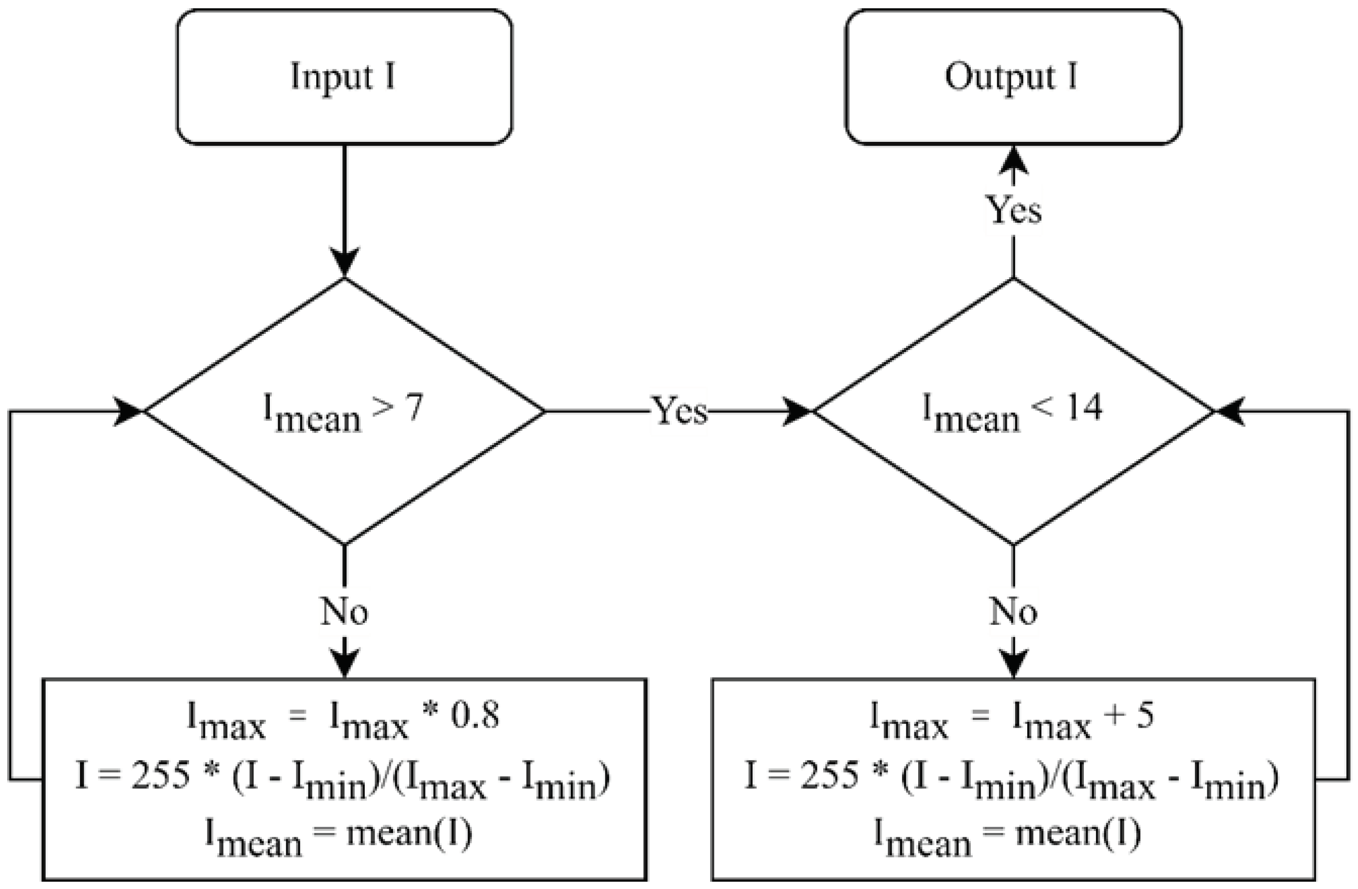
19] for brightness pre-processing. This method uses a linear transformation to adjust the dynamic range of an image, with the objective of controlling the average intensity of each image within the range of (7, 14). The algorithm for the linear transformation is illustrated in
Figure 1. The region below the knees, which is uncommon for bone metastasis, was excluded from the calculation of BSI. To obtain the region above the knees, pixels beyond row 640 are eliminated, resulting in two views with a spatial resolution of 640 × 256 pixels each. Finally, the pre-processed AP (anterior-posterior) and PA (posterior-anterior) view images were horizontally merged, generating images with a spatial resolution of 640 × 512 pixels.
Figure 1.
Flowchart of brightness normalization.
Figure 1.
Flowchart of brightness normalization.
2.4. Background Removal
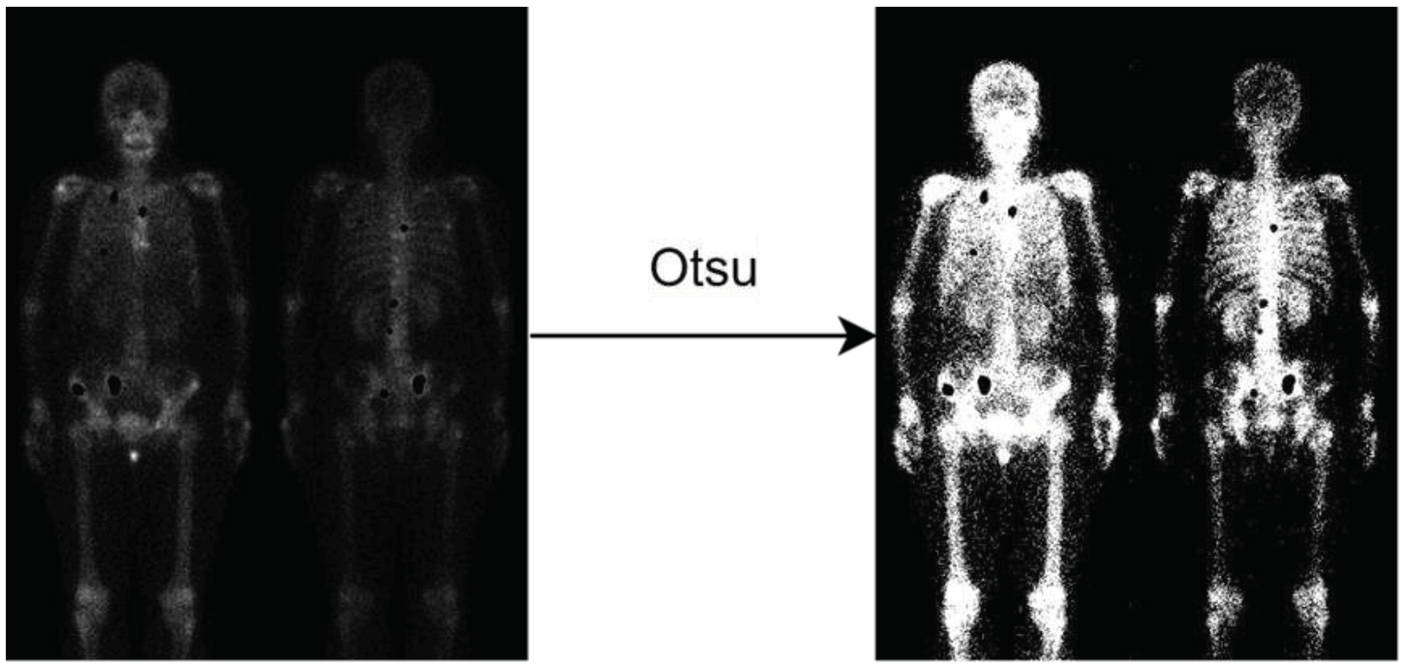
Given that the background of bone scan images predominantly consists of air, training on the air regions would generate meaningless results. Thus, a pre-process is used to eliminate the air regions from the images. This is achieved by applying Otsu thresholding [
28] to the non-metastatic regions, allowing for the automatic determination of the optimal threshold to remove the air regions and generate a mask specifically for the non-metastatic class, as shown in
Figure 2.
Figure 2.
Illustration of background removal. Notably, the metastasis hotspots are eliminated (the black holes), if this image has metastasis.
Figure 2.
Illustration of background removal. Notably, the metastasis hotspots are eliminated (the black holes), if this image has metastasis.
2.5. Adding Negative Samples
To solve the challenge of distinguishing between lesions and normal bone uptake hotspots, it is important to include normal images in the training dataset. This inclusion helps reduce the false positive rate and enhance the precision of the model. The mask for normal images can be generated using two different techniques: Otsu thresholding and negative mining.
The first approach involved generating a mask for non-metastatic samples by directly applying Otsu thresholding. This process can be applied on both normal images without metastasis or metastatic images. The Otsu thresholding finds a threshold to distinguish uptake regions from air, thus creating the non-metastatic class. Notably, the metastatic regions must be excluded manually if we are processing an image with metastasis. The second approach, known as negative mining [
19], utilizes a two-step process. Initially, the model is trained with bone metastasis images. Subsequently, this trained model is used to make predictions on normal images. Any output predictions on the normal images are for sure to be false positives and collected as the non-metastatic class. Negative mining offers the advantage of automatically generating negative samples without the need for manual annotation by experts, thereby saving time and effort. Additionally, negative mining focuses on areas where the model is prone to making mistakes, enabling error review and subsequent model improvement.
2.6. Transfer Learning
Transfer learning is a widely used technique in neural networks to increase their performance. Before applying transfer learning, two crucial factors need to be considered: (1) the size of the target dataset and (2) the similarity between the target dataset and the pre-training dataset.
In this study, a relatively small dataset is utilized, and it is anticipated that pre-training with a dissimilar dataset would have limited effectiveness. Consequently, we select a pre-training dataset comprising highly similar bone scan images from the prostate cancer. Subsequently, fine-tuning is performed on the model using the target dataset, which consisted of breast cancer bone scan images. By leveraging transfer learning and selecting a pre-training dataset that closely aligned with the target dataset, we aim to capitalize on the shared characteristics between the two datasets, thereby improving the model’s performance on the specific task at hand.
2.7. Data Augmentation
Neural networks (NNs) have demonstrated impressive performance in various computer vision tasks. However, to avoid overfitting, NNs typically require a substantial amount of training data. However, overfitting occurs while an NN excessively matches a specific dataset, whereas limiting its ability to generalize onto new test data. Medical images for annotations are often time-consuming so limited in training samples. Therefore, to solve the data scarcity and mitigate overfitting, data augmentation techniques are required.
In this study, we utilize two data augmentation techniques: brightness adjustment and horizontal flipping. For brightness adjustment, a linear transformation process like the brightness normalization shown in
Figure 1 is applied. The average brightness value (
m) of the original images served as a reference for adjusting the brightness. By setting the brightness range to (
m - 5,
m + 5), six additional brightness values were generated within this range, resulting in a total of seven brightness levels when combined with
m. Subsequently, the images corresponding to these seven brightness levels are horizontally flipped. Consequently, the dataset size is effectively augmented by a factor of 14.
2.8. 10-Fold Cross-Validation
To reduce the impact of a single random split and evaluate the model’s generalization performance on independent test data, we conduct 10-fold cross-validation for performance evaluation. The positive samples are divided into ten parts, with eight parts used for training, one part for validation, and one part for test, respectively in each fold. Additionally, the negative samples are included in the training set of each fold. Consequently, the model is trained on these ten subsets of data, and the results are averaged to obtain a comprehensive assessment of the model’s performance. This approach ensures a reliable evaluation and provides insights into the model’s effectiveness across different subsets of the dataset.
2.9. Neural Network Model
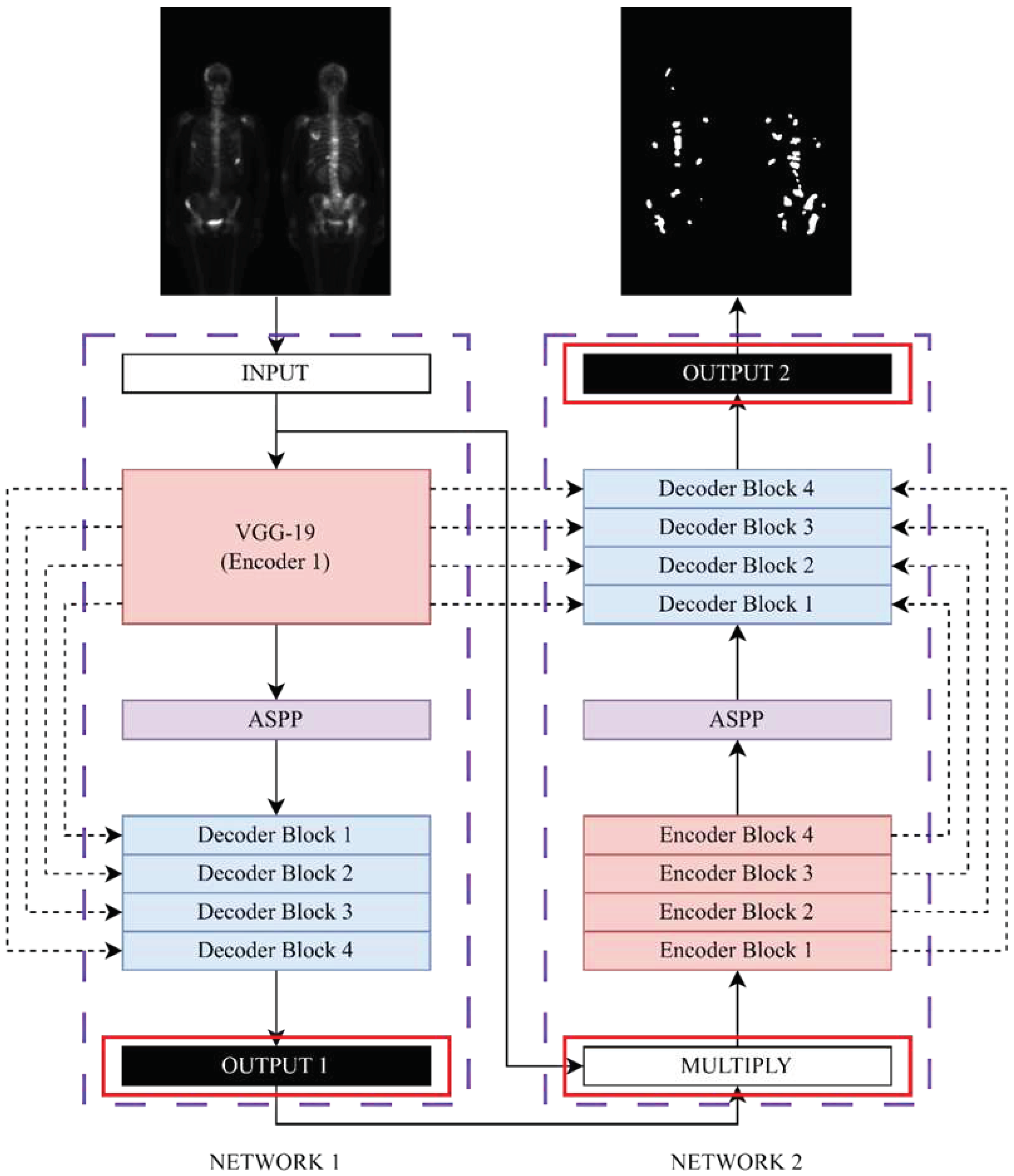
In this study, we modify Double U-Net model. The original Double U-Net architecture is developed for binary segmentation tasks, requiring modifications to adapt it for multi-class segmentation purposes. The modified Double U-Net architecture, as illustrated in
Figure 3, is utilized in this study. Specifically, the activation functions for OUTPUT 1 and OUTPUT 2 are changed to softmax to facilitate multi-class segmentation. Additionally, the original input image is multiplied with each output class, resulting in separate images that served as inputs for NETWORK 2. This modification enables the model to handle multi-class segmentation efficiently.
Figure 3.
The modified architecture diagram of Double U-Net.
Figure 3.
The modified architecture diagram of Double U-Net.
2.10. Loss Function
The selection of an appropriate loss function is a critical aspect in the design of deep learning architectures for image segmentation tasks, as it greatly impacts the learning dynamics of the algorithm. In our study, we consider two loss functions: the Dice loss (Equation 1), as originally proposed in [
25], and the Focal Tversky loss (Equation 2). By comparing these loss functions, we aim to explore their respective influences on the model’s performance in the context of our specific task.
The Dice coefficient is a widely adopted metric in computer vision for assessing the similarity between two images. In our study, we utilize a modified version of the Dice coefficient known as the Dice loss, which served as a loss function for our model.
where y is true value, and p is the predicted outcome.
The Focal Tversky loss is particularly well-suited for solving highly imbalanced class scenarios. It incorporates a γ coefficient that allows for the down-weighting of easy samples. Additionally, by adjusting the α and β coefficients, different weights can be assigned to false positives (FP) and false negatives (FN).
where γ = 0.75, α = 0.3, and β = 0.7.
4. Discussion
In this study, the vanilla Double U-Net architecture served as the baseline model for performance comparison. Subsequently, several optimization techniques are used to better the model. These techniques encompass adding negative samples (using Otsu thresholding), transfer learning, and data augmentation. Furthermore, the performance of different loss functions is compared. However, not all optimization methods result in improvement in performance. We discuss them in the following.
Among all the optimization methods, background removal is the most significant technique in improving the model’s performance. In bone scan images, the background mostly consists of air, which is unnecessary and irrelevant information. Extracting features from the air region would lower the model’s performance and waste computational resources. Applying Otsu thresholding can easily remove the air background. This method generates significant improvement without manual labeling, which is time-consuming.
In comparison from F1-score in
Table 2, the Otsu thresholding method shows slightly better than the negative mining method. We think that this might be due to the insufficient number of negative samples, compare to the area made by background removal as shown in
Figure 2. In the future, we plan to add more negative samples and further investigate the negative mining method to validate our assumption. The combination of background removing and negative mining would also a possible way to try.
In reference [
19], the task involves lesion detection and classification of three classes: metastatic, indeterminate, and normal hotspots. They use bounding boxes to define the region. The background removing we propose here cannot be applied to their application, since our task is semantic segmentation on bone metastatic lesions. In general, the negative mining technique reduces false positives, with the sacrifice of slight sensitivity. The difference in tasks between the two studies may have contributed to the variation in the effectiveness of negative mining.
Data augmentation is a commonly used technique to improve the robustness of deep learning models by generating new data samples from existing ones. It can solve data scarcity and alleviate overfitting issues. In our study, we utilize two data augmentation methods: brightness adjustment and horizontal flipping. However, the model performance is not better. Data augmentation has a smaller impact on more complex network models [
29]. In addition to the brightness adjustment and horizontal flipping used in our study, there are other methods such as geometric transformations, color space augmentation, random erasing, feature space augmentation, and generative adversarial networks [
30]. However, not all augmentation method is suitable to our study.
Apart from data augmentation, regularization methods specific to the model architecture, such as dropout, batch normalization, one-shot, and zero-shot learning algorithms, can effectively alleviate overfitting issues. In the Detectron2 and Scaled-YOLOv4 models [
31], using the same data and data augmentation methods, the two models exhibited significant differences in performance. The former achieves better results after data augmentation, while the latter obtains worse results. This indicates that the effectiveness of data augmentation is greatly influenced by the model architecture. Due to computational cost considerations, our study only uses brightness adjustment and horizontal flipping. In the future, we need to explore different data augmentation methods to find the optimal combination for the target dataset and network model.
In this study, we have tried Dice loss and Focal Tversky loss, and the latter generates better results. The selection of loss function plays a crucial role in model performance. For complex tasks like segmentation, there is no universally applicable loss function. It largely depends on the properties of the training dataset, such as distribution, skewness, boundaries, etc. For segmentation tasks with extreme class imbalance, Focal-related loss functions are more appropriate [
32]. Additionally, since the vanilla Double U-Net model has a higher precision than sensitivity, we are keen to use Tversky-related loss functions to balance the false positives (FP) and false negatives (FN) rates. Therefore, we adopt Focal Tversky loss as the compared loss function. In the future, further exploration and research can be conducted on the selection of optimizer.
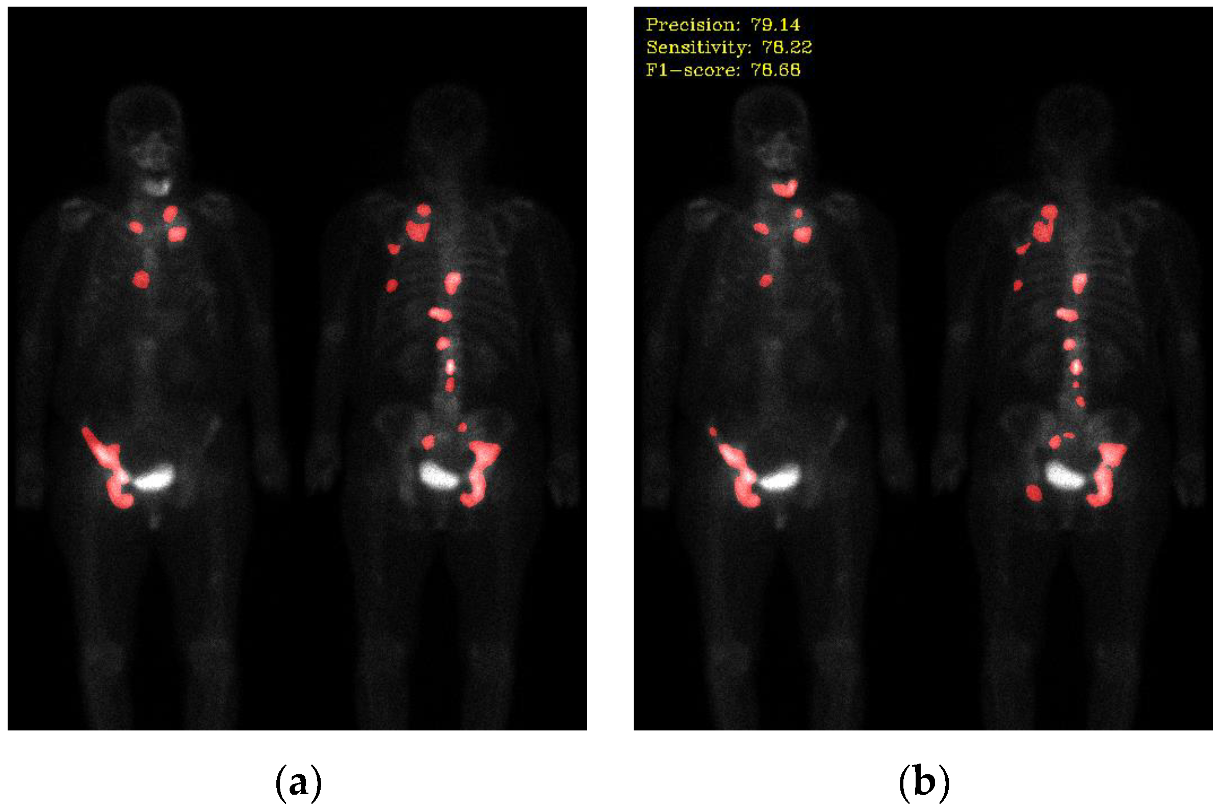
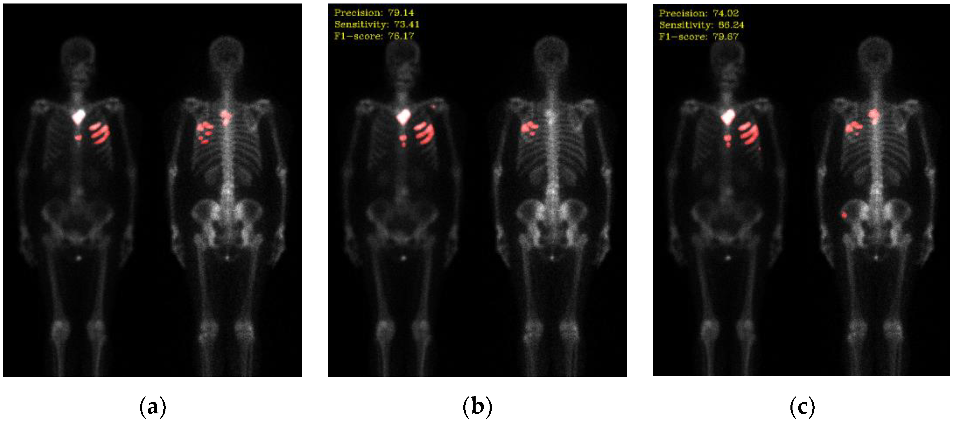
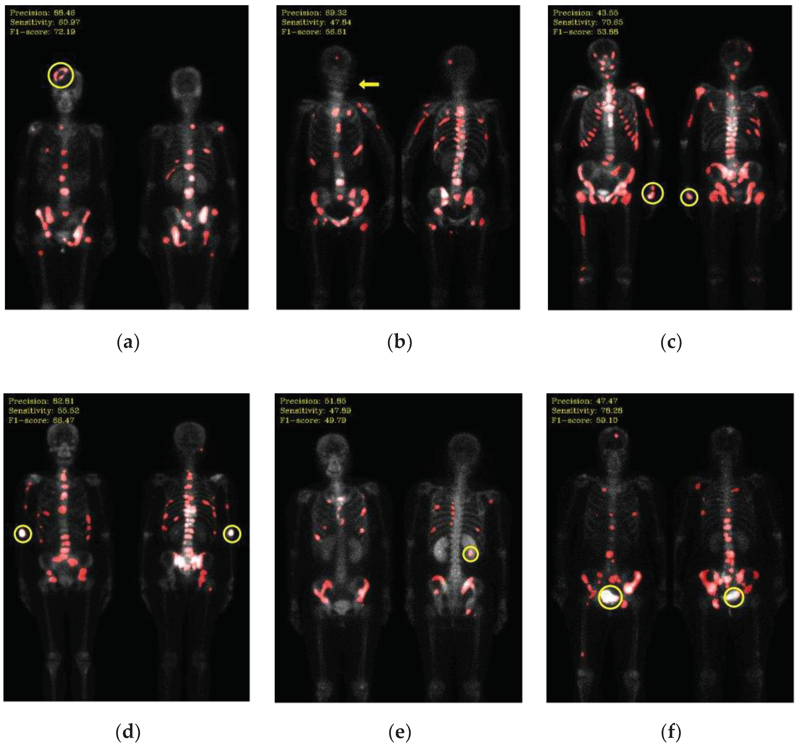
Not all hotspots in bone scan images represent bone metastases; normal bone absorption, renal metabolism, inflammation, and injuries can also cause hotspots in the images, leading to false positives in segmentation. In addition to the inherent imaging principles of bone scan images that make training the model challenging, the presence of artifacts in the images is also a crucial factor leading to misclassification. Examples of such artifacts include high-activity areas like the kidneys and bladder, the injection site of the radioactive isotope, and motion artifacts, as shown in
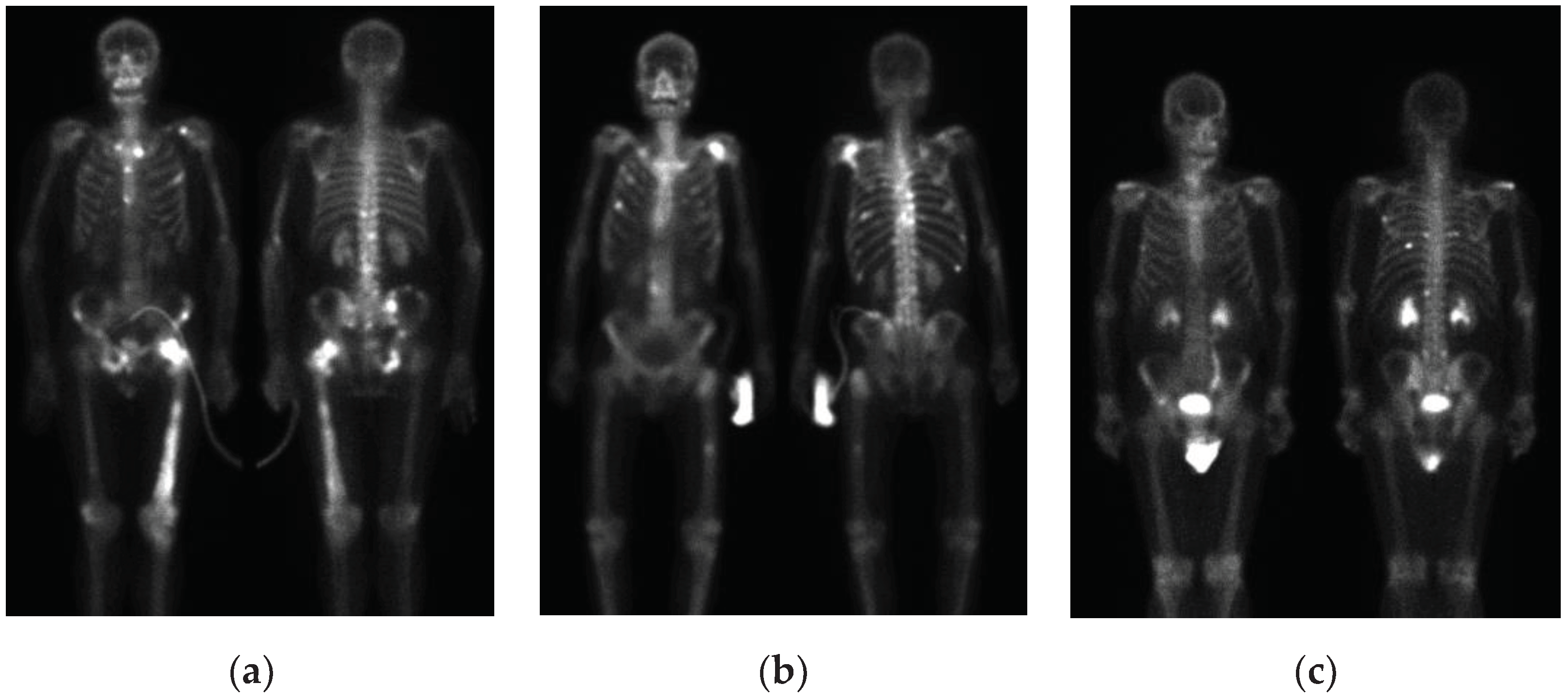
Figure 6. Apart from artifacts in breast cancer images, prostate cancer bone scan images also exhibit high-activity artifacts from catheters, urine bags, and diapers, as shown in
Figure 7. In the future, appropriate removal can be applied to minimize the impact from artifacts, or additional classes such as benign lesions and artifacts can be introduced to train the model more accurately.
Figure 6.
Mis-segmentation of non-metastatic lesions. (a) Bone fracture (head region) (precision: 88.46, sensitivity: 60.97, F1-score: 72.19); (b) motion artifact (head region) (precision: 69.32, sensitivity: 47.84, F1-score: 56.61); (c) injection site (wrist) (precision: 43.55, sensitivity: 70.65, F1-score: 53.88); (d) injection site (elbow) (precision: 82.81, sensitivity: 55.52, F1-score: 66.47); (e) kidney (precision: 51.85, sensitivity: 47.89, F1-score: 49.79); (f) bladder (precision: 47.47, sensitivity: 78.28, F1-score: 59.10).
Figure 7.
Artifacts in bone scan images of prostate cancer. (a) Catheter; (b) urinary bag; (c) diaper.
Figure 7.
Artifacts in bone scan images of prostate cancer. (a) Catheter; (b) urinary bag; (c) diaper.
The image pre-processing methods used in this study have significantly improved the model. Cheng et al. proposes a pre-processing method where the original images are combined into a 3D image to alleviate the issue of spatial connectivity loss [
19]. View aggregation, an operation applied to bone scan images, are used to enhance areas of high absorption [
24]. This method enhances lesions that appear in both anterior and posterior view images and maps lesions that only appear in either anterior or posterior view images. In the future, we can explore additional image pre-processing methods.
Due to the limited number of the dataset in house in this study, the model generalization is limited, and the training process may suffer from biases and limitations. The collaboration with other medical centers can be established to obtain more diverse and abundant data, thereby enhancing the model performance and generalization capability.
