Technical Note: Using Computer Vision’s Pixel Segmentation to Detect Beef Cattle Feeding Behavior

There is a need for cost-effective and non-invasive methods of monitoring feeding behavior in livestock operations, considering the significant impact of feed costs on economic efficiency and assisting in detecting health issues of group-fed animals. This paper proposes using deep learning-based computer vision techniques to detect pen-fed beef cattle feeding behavior using Mask Region-based Convolutional Neural Network (RCNN). A deep learning model was pre-trained on the Common Objects in Context (COCO) dataset to generate cattle instance segmentation. Manually defined feed bunk polygons are compared with these segmentation masks to derive feeding time for each bunk. A full day’s worth of video data and the corresponding physical sensor data are collected for the experiment. By benchmarking the computer vision detected data with physical ground truth over random time segments from morning to evening (thus various lighting conditions), the optimal thresholds for Mask RCNN are determined to be 0.7 for bounding boxes and 0.1 for masks. Using these parameters. The reports suggest that the computer vision system achieved a precision of 87.2% and a recall of 89.1%, signifying precise detection of feeding events. Our study, to the best of our knowledge, was one of the first investigations of instance segmentation on feeding time sense, which combines deep learning methods with traditional computer vision logistics, reporting on feeding time data collection and processing, camera testing and adjustment, and performance evaluation. Future research directions include computer vision applied in feed grading and animal re-identification for individual production analysis.

Keywords:

Subject: Biology and Life Sciences - Animal Science, Veterinary Science and Zoology

Introduction

The increasing incomes, expanding population, urbanization in various regions, and dietary changes in emerging countries have led to an unprecedented global demand for livestock products (Godde et al., 2018). Feed costs represent a significant portion (65-75%) of operational expenses in beef operations, making feed efficiency crucial for economic impact (Tedeschi et al., 2021). Thus, the scientific community must develop ways to increase production while maintaining or improving profitability and sustainability concurrently (Tedeschi and Beauchemin, 2023). Precision Livestock Farming (PLF) systems, incorporating a wide range of sensors to access production-related information, can potentially aid livestock producers’ livestock management (Banhazi et al., 2012). However, accurate scales are not widely applied in beef operations due to high cost and maintenance requirements (Wang et al., 2006). Besides, radio frequency identification sensors are needed to track individual animals, which requires frequent installation and maintenance (Halachmi et al., 2019).

Deep learning-based computer vision has experienced significant advancements driven by the increasing power of computers and neural network developments. Deep Convolutional Neural Network (CNN) algorithms can extract meaningful features, including shape, color, patterns, and more, from digital images (Krizhevsky et al., 2017). Combined with transformer attention head structure (Vaswani et al., 2017), algorithms such as DETR (Carion et al. 2020) are currently gaining popularity. Most CNN algorithms utilize the deep neural network to learn the high dimensional relationships between the digital input matrix and numerical output values for various tasks. For instance, ResNet (He et al., 2016) and VGG series (Simonyan and Zisserman, 2014) for image classification. YOLO series (Redmon et al., 2016), RetinaNet (Lin et al., 2017), and SSD (Liu et al., 2016) for object detection with bounding boxes. Mask RCNN (He et al., 2017) and SegNet (Badrinarayanan et al., 2017) for pixel segmentation. GAN (Goodfellow et al., 2014) and its variations for image generation.

Computer vision has a lot of applications in PLF (Tedeschi et al., 2021), including phenotyping, body measurements, production valuation, and animal tracking and behavior analysis (Fernandes et al., 2020). Li et al. (2017) investigated traditional statistic tools and deep learning methods to re-identify dairy cows with up to 99.6% precision. However, this method requires tailhead images which are somewhat challenging to take. Cominotte et al. (2020) tested four predictive approaches including multiple linear regression, least absolute shrinkage and selection operator, partial least squares, and artificial neural networks to estimate the livestock body weight and average daily gain using computer vision, with high accuracy (root mean square error of prediction of 0.02 kg/d). However, these methods require a particular top-down view and head-tail image for binary segmentation as pre-processing. For detailed animal reconstruction, Jakab et al. (2023) used diffusion structure to reconstruct 3D models from 2D images of animals for various following works. Li et al. (2019) developed a dataset for cattle pose estimation, containing 2,134 images of dairy and beef cattle on multiple poses under natural conditions. They trained a pose model using this dataset and achieved a remarkable PCKh mean score of 90.39% for 16 joints, with a threshold of 0.5. However, there is little work on feeding time analysis. Bresolin et al., (2023) labeled 2,209 images and trained an object detection algorithm on that to detect the feeding behavior. This work showed promising identification (benchmarked with manual labels) results but require manual labeling for different animal and bunk arrangements. Guo et al. (2021) designed a bi-directional gated recurrent unit to classify cattle behaviors, including exploring, feeding, grooming, standing, and walking. The overall F1 scores of such models are 82.16% (calf) and 79.32% (adult cow). Besides these two works, there is a lack of feeding behavior sensing based on computer vision signals.

Computer vision systems offer cost-effective and non-invasive monitoring of animals, capturing a wide range of behaviors with rich data. Deep learning-based computer vision techniques can extract meaningful information from digital images and classify, localize, and segment targets at the pixel level (LeCun et al., 2015) that can be used to monitor feeding behavior, health issues, and metabolism and energy utilization in beef cattle (Novais et al., 2019, Tedeschi et al., 2021). Our study proposes the application of a Mask Region-based Convolutional Neural Network (RCNN) (He et al. 2020) pre-trained on Common Objects in Context (COCO) dataset (Lin et al. 2014) and compares the pixel segmentations with the predefined feed bunks to derive feeding time.

Material and methods

Videos are made up of frames at a specific rate, usually 30 Frames Per Second (FPS) for real-time, but sometimes lower to save space, especially in monitoring systems. We decompress the video and extract individual frames which serve as input for the computer vision model. In this research, we select the Mask RCNN model due to its capability to produce individual animal masks which allow the comparison between the animal and bunk shapes. 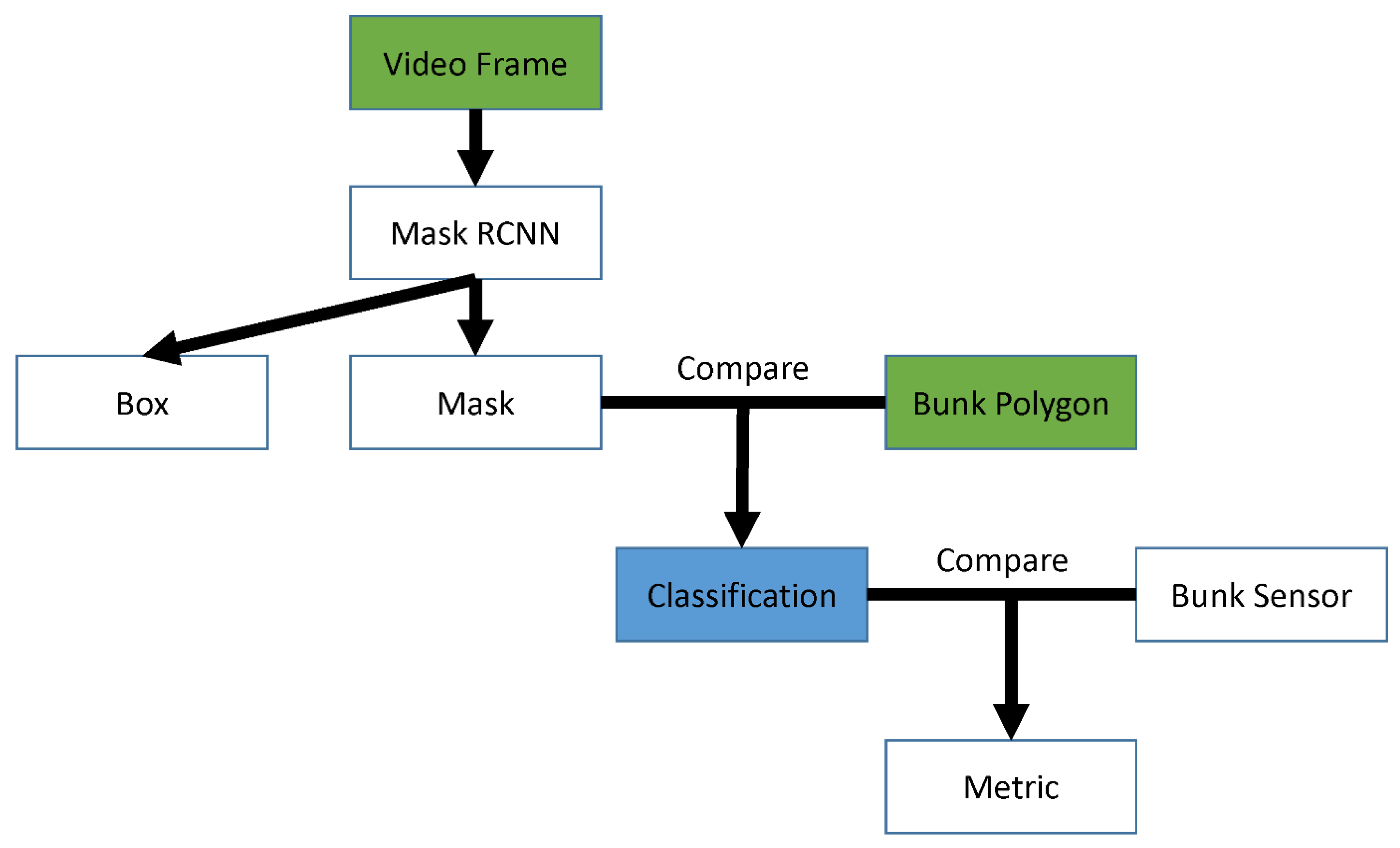Figure 1 shows the methodology of this research where the input is represented as green blocks and the blue blocks are the framework output. All the feed bunk polygons need to be manually defined by using free online tools, e.g., the VIA annotation tool (Dutta and Zisserman 2019). It is worth mentioning that this annotation should be done in the dimension of the full frame, not cropped frames. This task also requires the feeding bank opening to be both visible and substantial in size to facilitate accurate comparison.

Following the steps in Figure 1, each video frame is processed by the Mask RCNN model, which produces bounding boxes with pixel masks within them. Some low quality boxes and masks are dropped by using some optimized thresholds (more details in the subsection named Box and Mask Thresholds). Next, we compare each mask with each feeding bunk polygon geometrically. If there is an overlap between a mask and a polygon, we classify this as an indication of feeding at this bunk at the frame time T. The time T of such an event can be derived from the frame number, FPS, and the beginning time of the video. The computer vision classification records at all T are compared with the physical bunk sensor classification, and the following metric reports the performance.

Video and Feeding Data Collection

Thirty steers, 309 ± 4 kg of body weight, were randomly allocated into a pen for a feeding trial at the experimental research feedlot station located at Beef Cattle Systems from Texas A&M University, College Station, TX. Video data were recorded during the day by a camera (Microsoft LifeCam) at a resolution of 1280 x 720, on June 19th of 2022. The feeding events obtained were later converted to corresponding frames in the video to support frame level comparison. 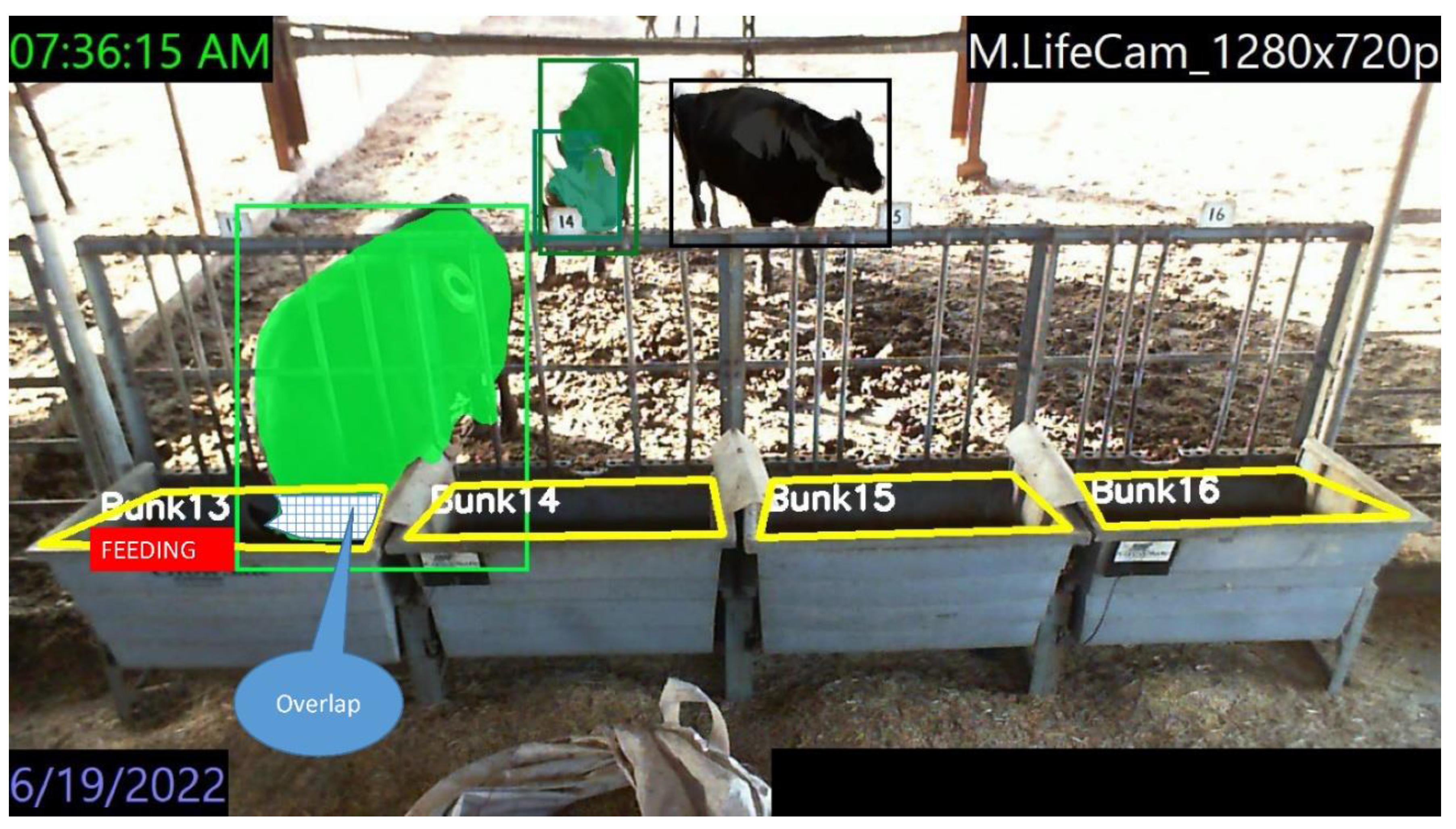Figure 2 provides one video frame example of a pen with four feeding bunks 13 to 16. Each feed bunk was manually marked with a yellow polygon for the CV analysis to identify the opening. The model, Mask-RCNN, first detects the animal with bounding boxes, then segments each pixel into the animal shape within the bounding box. Based on the segmentation results, each animal is highlighted with different color. When the colored pixels overlap with any yellow feed bunk polygons, area filled with grid in Figure 2, the time frame for that bunk is defined as feeding, and the corresponding bunk number is recorded. For instance, one cattle feeds at 7:36:15 AM at feed bunk 13.

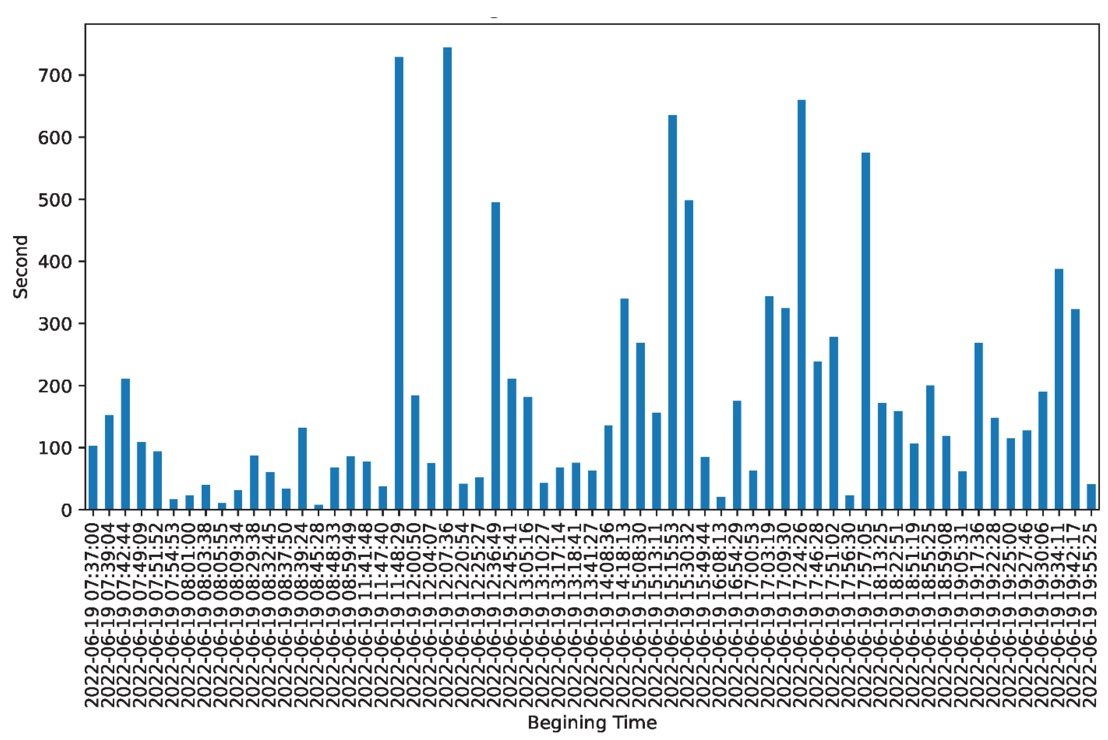
On the other hand, physical sensors are used to collect the feed time as shown in Figure 3-an example at bunk 15 on the same day. In this figure, the X-axis indicates the feeding starting time and the Y-axis represents the duration in seconds. The ultimate goal is to produce a time series that is as close as possible to this figure for each bunk. There is no records if there is no feeding. According to this figure, longer and more frequent feedings happened after 12:00.

Mask RCNN

Each video frame is a digital image with red, green, and blue channel pixels, which is a multi-dimensional matrix. Each pixel has a value ranging from 0 (darkest) to 255 (brightest) to represent the light intensity reflected by objects. The camera resolution means how many pixels are recorded, e.g., 1280 (width) × 720 (height) = 921,600 pixels. This matrix input is passed through multiple layers, each applying filters and convolutional computations. The network may also include pooling layers to resize the input and handle object movements. The final layer, a concatenation of the previous convolutional structure, is converted into a tall vector that represents the output. For example, in Mask RCNN, the output includes a list with X and Y coordinates and the confidence probability for bounding boxes that the system detects as corresponding to objects. Within each bounding box, the segmentation head classifies each pixel within the bounding box to determine if it belongs to the object. It provides the shape and instance segmentation of each object, which is crucial for comparing the shape of the cattle and the feeding bank, as shown in Figure 2.

The Mask RCNN’s weights are adjusted through multiple iterations using a large dataset called common objects in context (COCO) (Lin et al. 2014), developed by Microsoft, which contains 80 different common objects or classes. The weight optimization process aims to minimize the error between the manually labeled data and the predicted bounding boxes and segmentation. This process is named backpropagation (Yann LeCun et al. 1988). The final optimized model, along with its weights, is what we use in our system. Pre-trained versions of this model are readily available on various platforms such as Pytorch and free to use. It’s important to note that not all 80 classes such as car, person, airplane, etc, in the COCO dataset are used. We are primarily interested in the class for cows. The COCO dataset provides examples of cows that may not exactly match the breed and appearance of the cattle in our experiment, but they share similarities. This exploratory work allows us to test the preliminary applications.

Prediction Adequacy

Based on the frame rate (10 FPS in this research) and the video’s starting time, we calculate the corresponding time T for each frame. For each bunk at the time T, we compare the computer vision (CV) and bunk sensor measurements, which serve as the ground truth (GT). For instance, a feeding behavior is sensed at T1 for 10 seconds. Given the FPS=10, a total of T1 to T100 is marked as feeding for GT. To avoid confusion, we only use the abbreviation of CV and GT for metric calculation. Each CV and GT comparison is determined as true positives (TP), false positives (FP), false negatives (FN), and true negatives (TN), as shown in Table 1. A TP case occurs when a bunk in a frame is predicted as feeding aligns with the GT classification of feeding. On the other hand, an FP case arises when the CV model mistakenly identifies a bunk in a frame as feeding, despite GT indicating no feeding. TN represents cases where both CV and GT classify a bunk in a frame as not feeding, while an FN occurs when the CV suggests a bunk in a frame is not feeding, but the GT indicates feeding.

For all time T, we can compute the precision, recall, and overall performance (F1 score) for one bunk using Equations 1 to 3. Precision is the proportion of true positives out of all positive predictions (Eq. [1]), recall is the proportion of true positives out of all actual positive instances (Eq. [2]). Because this is a binary classification problem, we also report the F1 score (Eq. [3]), which is a balanced measure of the model’s precision and recall.

P r e c i s i o n = \frac{T P}{T P + F P}

(1)

R e c a l l = \frac{T P}{T P + F N}

(2)

F 1 = \frac{2 * (p r e c i s i o n * r e c a l l)}{p r e c i s i o n + r e c a l l}

(3)

Results and discussion

Experiment

In this experiment, the researchers utilized Python and popular computer vision packages like OpenCV, PyTorch, and related input/output tools. Python was chosen due to its comprehensive deep learning capabilities and community support, which are lacking in other programming languages. The code was executed on the High Performance Research Computing (HPRC) infrastructure at Texas A&M University. Specifically, the A100 GPU was employed to reduce processing time significantly but regular computer can also process long videos with skipping frames (e.g., one frame every second). 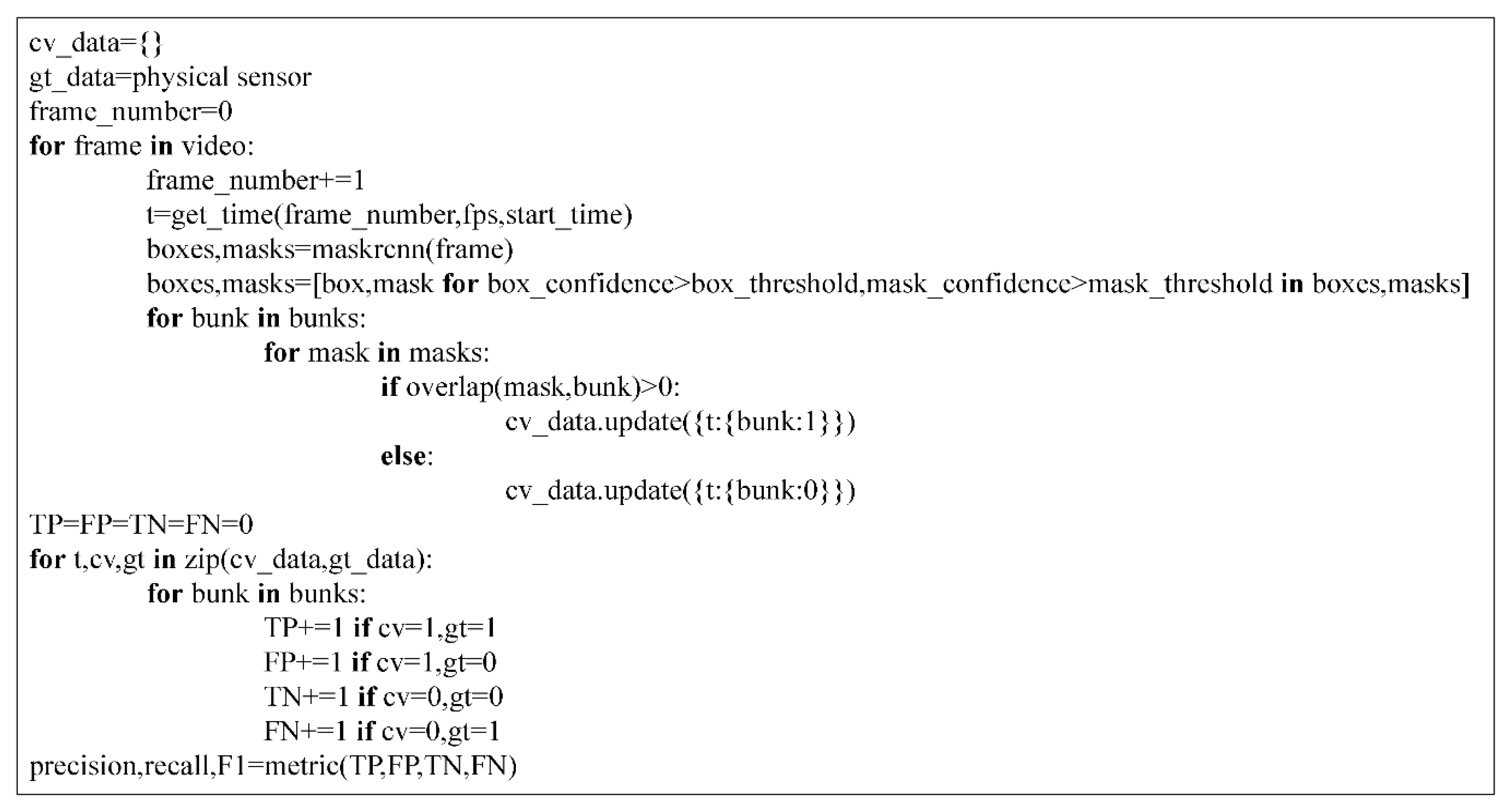Figure 4 depicts the pseudocode for the programs, which is an informal and human-readable representation of the algorithm. Pseudocode is not tied to any specific programming language and focuses on expressing the logic and structure of the code rather than the exact syntax. It allows programmers to plan, communicate, and understand algorithms before writing actual code.

The first part of the pseudocode initializes the necessary variables and data holders. The cv_data is an empty dictionary that will store the results of the computer vision analysis. gt_data represents the ground truth data obtained from the physical sensor. The frame_number variable is set to 0, indicating the initial frame. The pseudocode then enters a loop that iterates through each frame of the video. For every frame, the frame_number is incremented, and the corresponding time t is calculated using the get_time function. This function considers the frame number, FPS, and the start time to determine the time associated with the current frame.

Within the loop, the maskrcnn function is applied to the current frame to perform instance segmentation. This function returns two sets of data: boxes and masks with confidences. These results are then filtered based on confidence thresholds. Next, the pseudocode examines each bunk (predefined) and checks for overlap between each bunk and the masks. If there is an overlap between a mask and a bunk, a value of 1 is assigned to cv_data at the corresponding time t and bunk. Conversely, if there is no overlap, a value of 0 is assigned. This feature avoids duplicated counting. Moving on, the pseudocode focuses on evaluating the performance. It initializes variables for TP, FP, TN, and FN to 0. For each time t, computer vision prediction (cv), and ground truth (gt) in the cv_data and gt_data dictionaries, the pseudocode compares the predicted results with the ground truth. By iterating through each bunk, it increments the appropriate counters (TP, FP, TN, and FN) based on the conditions specified. Finally, the pseudocode invokes the metric function, which takes the TP, FP, TN, and FN values as inputs and calculates the precision, recall, and F1 score.

Box and Mask Thresholds

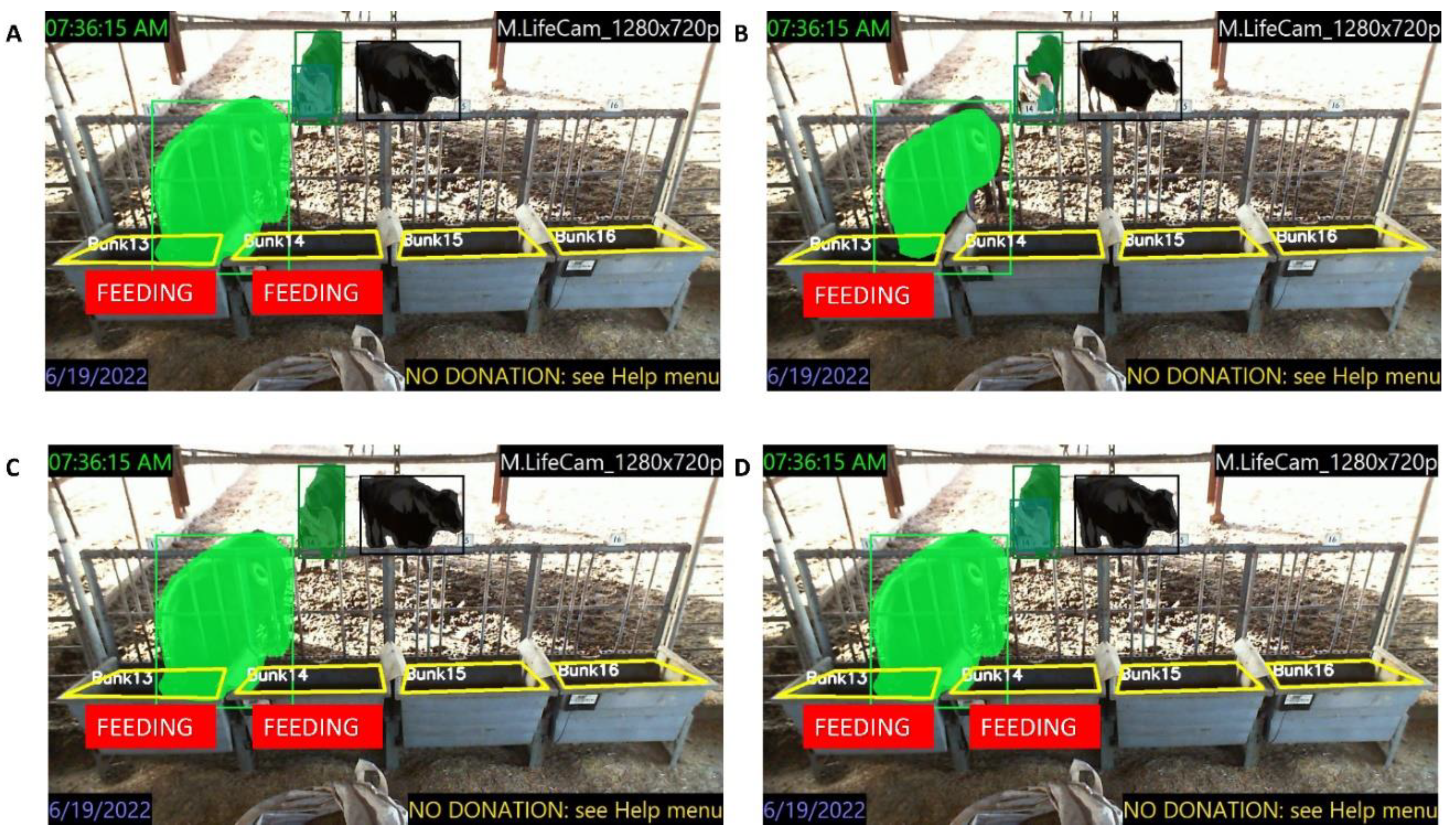
In generating the Mask RCNN results, each bounding box is assigned a score, and every pixel within that box is given a probability. Both these values range from 0 to 100%, indicating the model’s confidence level in classifying the box and the pixel. In practical terms, two thresholds exist for both the score and the probability to filter out detections with low confidence. As depicted in Figure 5, the effects of these two parameters are explored across a range from 0.1 to 0.9. The figure reveals that as the thresholds increase, fewer boxes and pixels are identified as the shape of a cattle, which leads to fewer feeding detections from the computer vision system. Conversely, setting low thresholds results in numerous predictions, including false detections. Thus, an experiment has been conducted to optimize the best combination of thresholds.

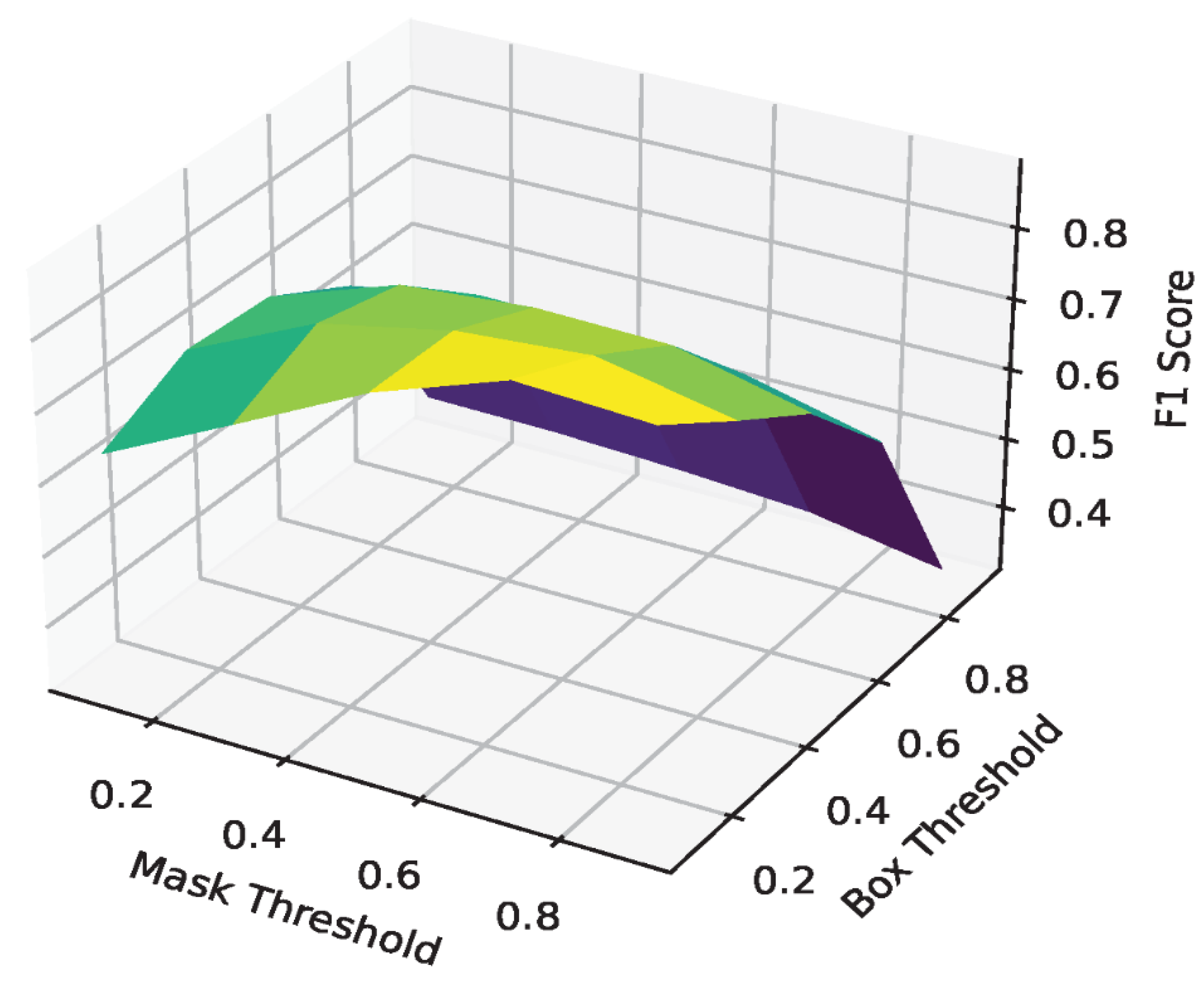
We randomly select 13 segments each lasting 2 minutes and 30 seconds (sampled from 7:00 to 19:00 to cover all lighting conditions) for the optimization process. In this experiment, an interval of 0.2 is used to loop through all box and mask thresholds, and the corresponding F1 scores are calculated and plotted. According to the resulting graph in Figure 6, the best threshold should be around 0.1 and 0.7 for box and mask, respectively. This selection is consistent with intuition because we want to have as many boxes as possible to consider all the castles, e.g., the false positive cases in the background will not decrease the performance. Next, we want to find very fine shapes of the animals to do the comparison. Too low a mask threshold will result in spilling segmentation hindering performance, e.g., Figure 5 (A) (C) and (D) bunk 14 has FP feeding signal.

Performance

After determining the best thresholds, all the video segments are processed using the optimum combination, e.g., 0.1 for box and 0.7 for mask. A total of 98,720 cases are classified as either feeding or not feeding by computer vision. To establish ground truth data, the feeding time records are converted into 98,720 cases with feeding and not feeding labels. This allows us to treat the problem as a binary classification task. Table 2 presents the total counts for each case in this experiment. The majority of cases are TP and TN, indicating good performance. Using equations 1, 2, and 3, and the values from Table 2, it is suggested that the computer vision system achieved a precision of 87.22% and a recall of 89.09%. These results imply a balanced performance of 88.15% F1 score.

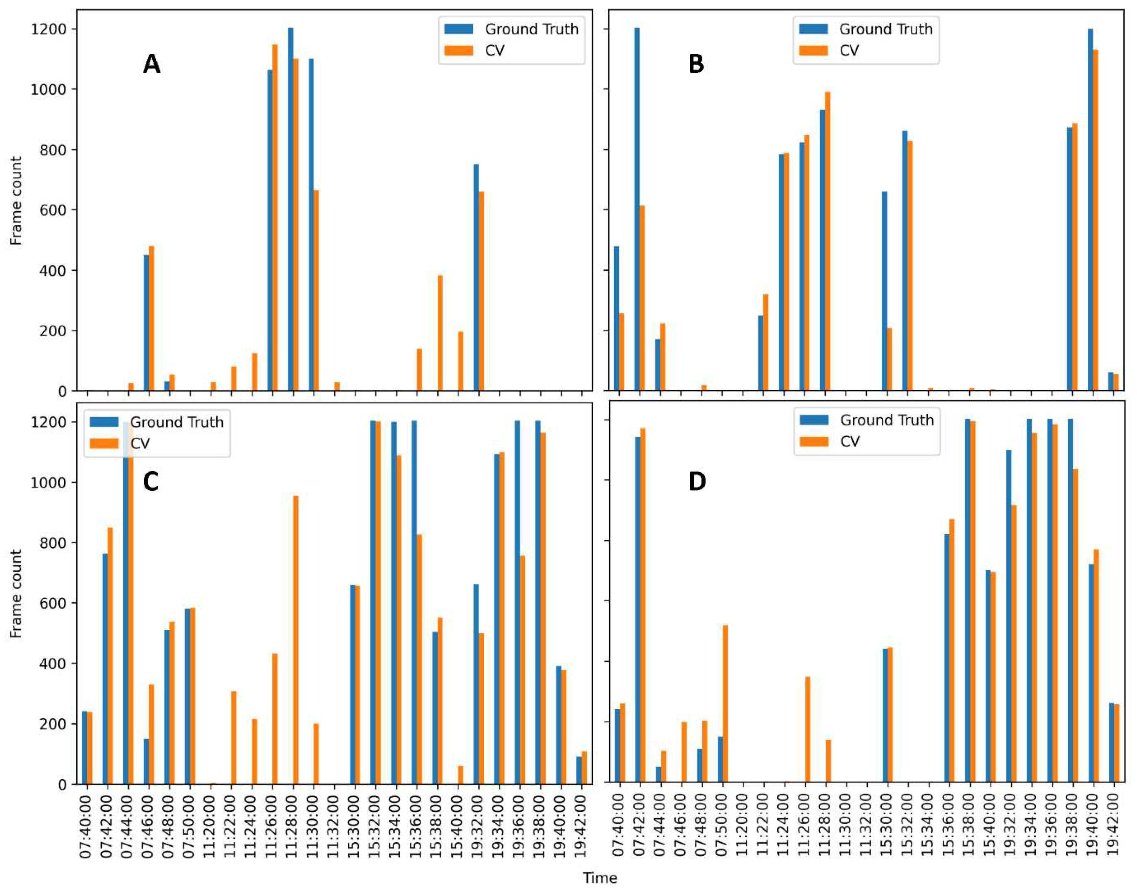
Figure 7 present a 40-minute comparison between the computer vision predictions and the ground truth data, focusing on two-minute intervals. We randomly select 4 (roughly 10-minute) time segments (7:41 - 7:51, 11:21 - 11:31, 15:30 - 15:40, 19:32 - 19:42) for the experiment. The vertical axis of the figure represents the number of frames classified as feeding, while the horizontal axis indicates the time in minutes. The data is aggregated with two-minute intervals, hence where minutes without feeding events have a height of zero, and minutes with continuous feeding have a height of 1200 frame count. All subfigures demonstrate a close alignment between the CV predictions and the GT data under various lighting conditions, i.e., from morning to night. Some bunks have more visits than others during different times. However, it is important to note that the CV predictions exhibit some noise, primarily due to FP masks.

Conclusion

In this research, we proposed the use of pixel segmentation and deep learning techniques, specifically Mask RCNN, for detecting feeding behavior in beef cattle. Each detected beef cattle mask was compared with predefined bunk polygons to determine feeding time in the camera pixel space. Next, the computer vision-generated feeding time data was compared with physical sensor data to measure the performance. The performance evaluation of the system demonstrated promising results with high precision and recall rates. The computer vision system achieved a precision of 87.22% and a recall of 89.09%, indicating accurate detection of feeding events. The optimum box and mask thresholds for Mask RCNN filtering were measured to be 0.1 and 0.7, respectively. The results indicate that computer vision can be applied to support detailed analysis for precision livestock farming management. Future research directions could include exploring feed grading and animal re-identification using computer vision signals that can contribute to enhanced monitoring and management.

Abbreviations

CNN = convolutional neural network, COCO = common objects in context, FPS =frames per second, PLF = precision livestock farming, RCNN = region-based CNN, CV=computer vision, GT=ground truth, TP=true positive, FP=false positive, TN=true negative, and FN=false negative.

References

Badrinarayanan, V., A. Kendall, and R. Cipolla. 2017. SegNet: A Deep Convolutional Encoder-Decoder Architecture for Image Segmentation. IEEE Trans. Pattern Anal. Mach. Intell. 39:2481–2495. Available from: https://www.ncbi.nlm.nih.gov/pubmed/28060704. [CrossRef]
Banhazi, T. M., L. Babinszky, V. Halas, and M. Tscharke. 2012. Precision livestock farming: precision feeding technologies and sustainable livestock production. International Journal of Agricultural and Biological Engineering. 5:54–61. Available from: https://research.usq.edu.au/item/q1yz0/precision-livestock-farming-precision-feeding-technologies-and-sustainable-livestock-production. [CrossRef]
Bresolin, T., R. Ferreira, F. Reyes, J. Van Os, and J. R. R. Dórea. 2023. Assessing optimal frequency for image acquisition in computer vision systems developed to monitor feeding behavior of group-housed Holstein heifers. J. Dairy Sci. 106:664–675. [CrossRef]
Carion, N., F. Massa, G. Synnaeve, N. Usunier, A. Kirillov, and S. Zagoruyko. 2020. End-to-End Object Detection with Transformers. In: Computer Vision – ECCV 2020. Springer International Publishing. p. 213–229. [CrossRef]
Cominotte, A. Cominotte, A., A. F. A. Fernandes, J. R. R. Dorea, G. J. M. Rosa, M. M. Ladeira, E. H. C. B. van Cleef, G. L. Pereira, W. A. Baldassini, and O. R. Machado Neto. 2020. Automated computer vision system to predict body weight and average daily gain in beef cattle during growing and finishing phases. Livest. Sci. 232:103904. Available from: https://www.sciencedirect.com/science/article/pii/S1871141319310856. [CrossRef]
Dorea, J. R. R., and S. Cheong. 2019. PSXI-2 A computer vision system for feed bunk management in beef cattle feedlot. J. Anim. Sci. 97:389. Available from: https://www.ncbi.nlm.nih.gov/pmc/articles/PMC6898560/. [CrossRef]
Dutta, A., and A. Zisserman. 2019. The VIA Annotation Software for Images, Audio and Video. In: Proceedings of the 27th ACM International Conference on Multimedia. Association for Computing Machinery, New York, NY, USA. p. 2276–2279. [CrossRef]
Fernandes, A. F. A., J. R. R. Dórea, and G. J. de M. Rosa. 2020. Image Analysis and Computer Vision Applications in Animal Sciences: An Overview. Front Vet Sci. 7:551269. [CrossRef]
Godde, C. M., T. Garnett, P. K. Thornton, A. J. Ash, and M. Herrero. 2018. Grazing systems expansion and intensification: Drivers, dynamics, and trade-offs. Global Food Security. 16:93–105. Available from: https://www.sciencedirect.com/science/article/pii/S2211912417300391. [CrossRef]
Goodfellow, I., J. Pouget-Abadie, M. Mirza, B. Xu, D. Warde-Farley, S. Ozair, A. Courville, and Y. Bengio. 2014. Generative Adversarial Nets. In: Z. Ghahramani, M. Welling, C. Cortes, N. Lawrence, and K. Q. Weinberger, editors. Advances in Neural Information Processing Systems. Vol. 27. Curran Associates, Inc. Available from: https://proceedings.neurips.cc/paper_files/paper/2014/file/5ca3e9b122f61f8f06494c97b1afccf3-Paper.pdf.
Guo, Y., Y. Qiao, S. Sukkarieh, L. Chai, and D. He. 2021. Bigru-attention based cow behavior classification using video data for precision livestock farming. Transactions of the ASABE. 64:1823–1833. Available from: https://elibrary.asabe.org/abstract.asp?aid=52831. [CrossRef]
Halachmi, I., M. Guarino, J. Bewley, and M. Pastell. 2019. Smart Animal Agriculture: Application of Real-Time Sensors to Improve Animal Well-Being and Production. Annu Rev Anim Biosci. 7:403–425. doi:10.1146/annurev-animal-020518-114851. [CrossRef]
He, K., G. Gkioxari, P. Dollár, and R. Girshick. 2017. Mask r-cnn. In: Proc. IEEE Int. Conf. Comput. Vis. Venice, Italy. p. 2961–2969.
He, K., G. Gkioxari, P. Dollar, and R. Girshick. 2020. Mask R-CNN. IEEE Trans. Pattern Anal. Mach. Intell. 42:386–397. Available from: http://openaccess.thecvf.com/content_iccv_2017/html/He_Mask_R-CNN_ICCV_2017_paper.html. [CrossRef]
He, K., X. Zhang, S. Ren, and J. Sun. 2016. Deep residual learning for image recognition. In: Proc. IEEE Conf. Comput. Vis. pattern Recognit. IEEE, Las Vegas, NV, USA. p. 770–778.
Jakab, T., R. Li, S. Wu, C. Rupprecht, and A. Vedaldi. 2023. Farm3D: Learning Articulated 3D Animals by Distilling 2D Diffusion. arXiv [cs.CV]. Available from: http://arxiv.org/abs/2304.10535. [CrossRef]
Krizhevsky, A., I. Sutskever, and G. E. Hinton. 2017. ImageNet classification with deep convolutional neural networks. Commun. ACM. 60:84–90. [CrossRef]
LeCun, Y., Y. Bengio, and G. Hinton. 2015. Deep learning. Nature. Available from: https://www.nature.com/articles/nature14539. [CrossRef]
LeCun, Y., D. Touresky, G. Hinton, and T. Sejnowski. 1988. A theoretical framework for back-propagation. In: Proceedings of the 1988 connectionist models summer school. Vol. 1. p. 21–28. Available from: https://www.researchgate.net/profile/Yann-Lecun/publication/2360531_A_Theoretical_Framework_for_Back-Propagation/links/0deec519dfa297eac1000000/A-Theoretical-Framework-for-Back-Propagation.pdf.
Lin, T.-Y., P. Goyal, R. Girshick, K. He, and P. Dollár. 2017. Focal loss for dense object detection. In: Proc. IEEE Int. Conf. Comput. Vis. IEEE, Venice, Italy. p. 2980–2988.
Lin, T.-Y., M. Maire, S. Belongie, J. Hays, P. Perona, D. Ramanan, P. Dollár, and C. L. Zitnick. 2014. Microsoft coco: Common objects in context. In: Eur. Conf. Comput. Vis. Springer. p. 740–755.
Liu, W., D. Anguelov, D. Erhan, C. Szegedy, S. Reed, C.-Y. Fu, and A. C. Berg. 2016. SSD: Single Shot MultiBox Detector. In: Computer Vision – ECCV 2016. Springer International Publishing. p. 21–37. [CrossRef]
Li, W., Z. Ji, L. Wang, C. Sun, and X. Yang. 2017. Automatic individual identification of Holstein dairy cows using tailhead images. Comput. Electron. Agric. 142:622–631. Available from: https://www.sciencedirect.com/science/article/pii/S0168169917300649. [CrossRef]
Li, X., C. Cai, R. Zhang, L. Ju, and J. He. 2019. Deep cascaded convolutional models for cattle pose estimation. Comput. Electron. Agric. 164:104885. Available from: https://www.sciencedirect.com/science/article/pii/S016816991831874X. [CrossRef]
Novais, F. J., P. R. L. Pires, P. A. Alexandre, R. A. Dromms, A. H. Iglesias, J. B. S. Ferraz, M. P.-W. Styczynski, and H. Fukumasu. 2019. Identification of a metabolomic signature associated with feed efficiency in beef cattle. BMC Genomics. 20:8. [CrossRef]
Redmon, J., S. Divvala, R. Girshick, and A. Farhadi. 2016. You only look once: Unified, real-time object detection. In: Proc. IEEE Conf. Comput. Vis. pattern Recognit. IEEE, Las Vegas, NV, USA. p. 779–788.
Simonyan, K., and A. Zisserman. 2014. Very deep convolutional networks for large-scale image recognition. arXiv Prepr. arXiv1409.1556.
Tedeschi, L. O., P. L. Greenwood, and I. Halachmi. 2021. Advancements in sensor technology and decision support intelligent tools to assist smart livestock farming. J. Anim. Sci. 99. [CrossRef]
Vaswani, A., N. Shazeer, N. Parmar, J. Uszkoreit, L. Jones, A. N. Gomez, Ł. Kaiser, and I. Polosukhin. 2017. Attention is all you need. Adv. Neural Inf. Process. Syst. 30. Available from: https://proceedings.neurips.cc/paper/7181-attention-is-all.
Wang, Z., J. D. Nkrumah, C. Li, J. A. Basarab, L. A. Goonewardene, E. K. Okine, D. H. Crews Jr, and S. S. Moore. 2006. Test duration for growth, feed intake, and feed efficiency in beef cattle using the GrowSafe System. J. Anim. Sci. 84:2289–2298. [CrossRef]

Figure 1. Research Methodology.

Figure 2. Example of computer vision feeding sensing. Each feed bunk was manually marked with a yellow polygon. When there is an intersection between the bunk polygon and the grey cattle mask, that bunk is defined as feeding. Otherwise, there is no feeding.

Figure 3. Bunk 15 feeding time based on physical sensors on June 19th, 2022. X-axis represents the beginning time of feeding. Y-axis indicates the duration of the feeding in seconds.

Figure 4. Experiment pseudocode. The first section generates the computer vision feeding behavior data (cv_data) at each frame per bunk. The second section compares cv_data with the gt_data that is collected by a physical sensor to report precision, recall, and F1 score.

Figure 5. Pixel segmentation examples using different mask and box thresholds. (A) Mask 0.1 and box 0.1. (B) Mask 0.9 and box 0.1. (C) Mask 0.1 and box 0.9. (D) Mask 0.9 and box 0.9.

Figure 6. F1 scores under the different box and mask threshold combinations.

Figure 7. Comparison of CV and GT feeding frame count aggregated by 120 seconds (hence 1200 maximum count on the vertical axis) at the Mask RCNN thresholds of 0.1 for box and 0.7 for mask. Four time segments are 7:41 - 7:51, 11:21 - 11:31, 15:30 - 15:40, and 19:32 - 19:42 marked on the horizontal axis. (A) Bunk 13. (B) Bunk 14. (C) Bunk 15. (D) Bunk 16.

Table 1. Examples of computer vision (CV) and bunk sensor ground truth (GT) classification at time T.

	CV	GT	Case
T1	Feeding (1)	Feeding (1)	TP
T2	Feeding (1)	Not Feeding (0)	FP
T3	Not Feeding (0)	Feeding (1)	FN
T4	Not Feeding (0)	Not Feeding (0)	TN
Tn	…	…	…

Table 2. TP, FP, TN, and FN count for all four bunks.

GT\CV	Not Feeding	Feeding
Not Feeding	56,472	5,941
Feeding	4,205	32,102

Disclaimer/Publisher’s Note: The statements, opinions and data contained in all publications are solely those of the individual author(s) and contributor(s) and not of MDPI and/or the editor(s). MDPI and/or the editor(s) disclaim responsibility for any injury to people or property resulting from any ideas, methods, instructions or products referred to in the content.

© 2023 by the authors. Licensee MDPI, Basel, Switzerland. This article is an open access article distributed under the terms and conditions of the Creative Commons Attribution (CC BY) license (https://creativecommons.org/licenses/by/4.0/).

Copyright: This open access article is published under a Creative Commons CC BY 4.0 license, which permit the free download, distribution, and reuse, provided that the author and preprint are cited in any reuse.

MDPI Initiatives

Important Links

Choose an area of interest and we will send you notifications of new preprints at your preferred frequency.

Disclaimer

Technical Note: Using Computer Vision’s Pixel Segmentation to Detect Beef Cattle Feeding Behavior

Abstract

Abbreviations

References

MDPI Initiatives

Important Links

Subscribe