The present paper provides a new definition for dual spline curves in a geometric intuitive way based on adaptive curve refinement techniques. The dual spline is an implementation of the interpolatory subdivision scheme for curve modeling, which is comprised of polynomial segments of different degrees. Specially, the dual spline curves are mainly aims to solve the difficult geometry defeaturing problems in the existing computer-aided technology. Dual spline curves maintain various desirable properties of conventional curve modeling methods, such as local adaptive subdivision, high interpolation accuracy and convergence, continuous and discontinuous boundary approximation. By adding fictitious and intrinsic nodes inside or at the vertices of interpolation elements, the dual spline is flexible and convenient for approximating a set of ordered points or discrete segments. Combined with the Lagrange interpolation polynomial and meshless method, the proposed approach is capable of approximating the non-smooth boundary for geometry defeaturing. Experimental results are given to verify the validity, robustness, and accuracy of the proposed method.

Keywords:

Subject: Computer Science and Mathematics - Geometry and Topology

1. Introduction

Reverse engineering is an attractive technique for computer-aided design (CAD) model construction from the scattered points of an existing solid [1,2]. Curve modeling has emerged as a powerful technology to treat experimental data points, which is concerned with fitting the given point set to a suitable mathematical model [3,4,5]. The existing geometric model in reverse engineering can be measured using various scanning and probing techniques. No matter what curve modeling techniques are applied, geometry noises and incomplete data points are often unavoidable in reverse engineering. Another critical difficulty in curve modeling is that measured points with the irregular format are tricky for desired curve construction [6,7]. For complicated geometries, curve modeling for automatic geometry repair is still a bottleneck in the field of computer-aided geometric design.

Various curve modeling methods have been proposed to eliminate the difficulties in dealing with solid modeling. Among all the representations, Non-Uniform Rational B-Spline (NURBS) has become the industrial standard for free-form curve construction [8]. 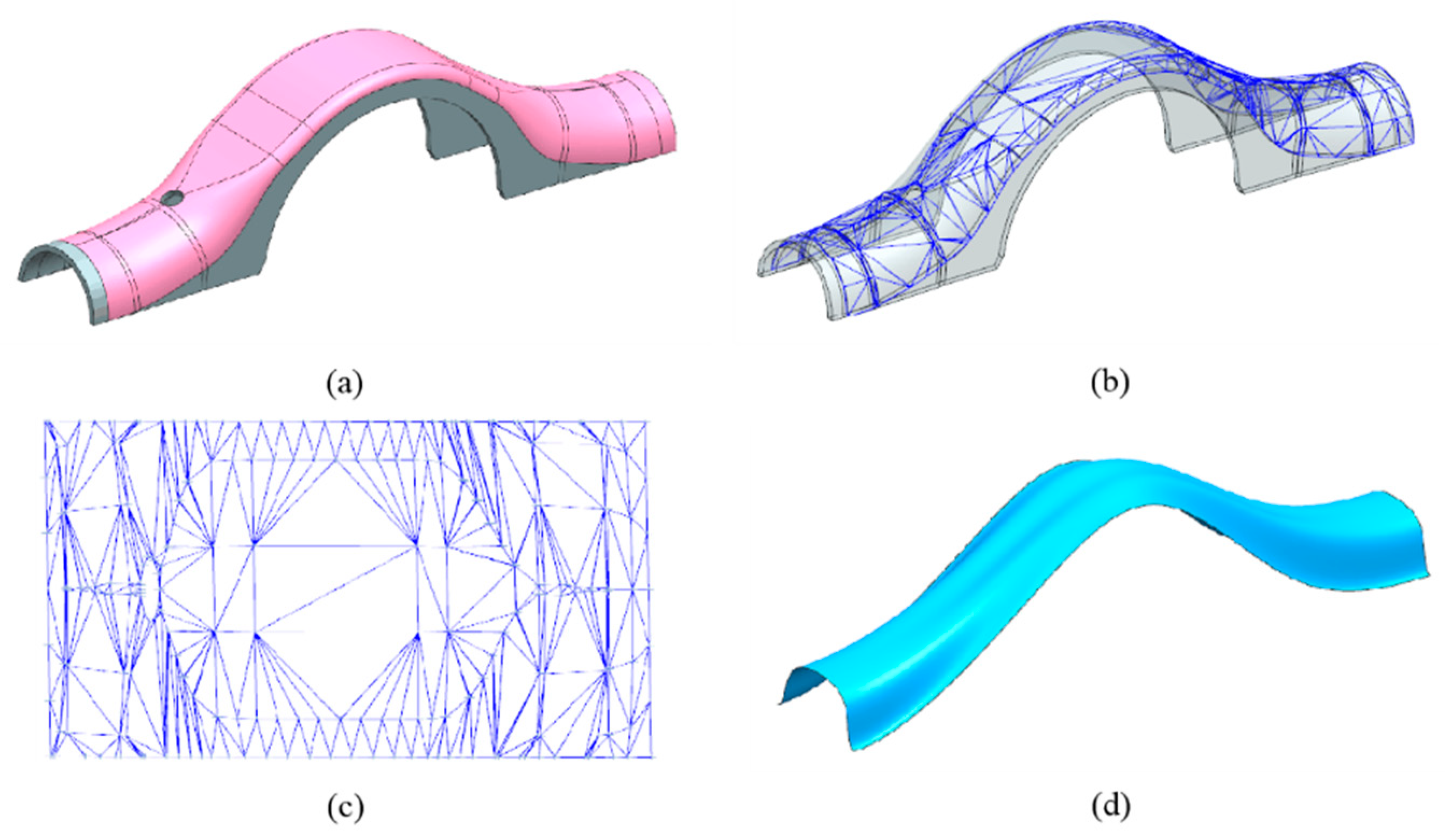For better adaptive curve construction, many different types of splines have been put forward for various curve modeling purposes, such as B-Spline [9], T-Spline [10], X-Spline [11], PH spline [12], B´ezier curves [13] and etc. In complicated solid modeling, there are plenty of lower-degree primitives and higher- degree free-form patches. Consequently, the conventional curve modeling methods are mathematically incapable of fulfilling the role of dealing with the geometry defeaturing problems. Suppose the lower-degree solid boundary is reconstructed by a few higher-degree patches, which will produce undesired geometry features and make them no longer to be primitives (see Figure 1). To construct a geometric model with complex topology. In that case, it is still a challenging task to keep the smoothness and continuity between the adjacent curved boundaries [14].

The alternative is to represent the solid boundary by subdivision methods [15,16], which is also a powerful and efficient technique to generate desired curves or surfaces. The subdivision scheme can be considered as the generalization of discrete modeling by spline representation, such as the Catmull-Clark subdivision [17], Doo-Sabin subdivision [18], Loop subdivision [19], and other classes of interpolatory subdivision schemes. The adaptive subdivision algorithm [20,21,22,23] is less cumbersome by defining the refinement rules to add new points as linear combinations of old ones. The process continues until the given terminating criteria for all discrete segments or patches are not met. Even more, when fitting a set of ordered points by the subdivision techniques, each segment can be considered an elementary mathematical problem. Arbitrary curve modeling by discrete segments can be controlled adaptively and efficiently within a prescribed tolerance.

This paper introduces a novel method to construct a dual spline curve from any given point set. By using extensive processing of dominant points, the dual spline is capable to produce better curve with the desired shape fidelity. The dual spline has many interesting properties, making it an efficient and powerful technique for shape modeling. The contributions and innovations of dual spline can be summarized in the following aspects:

(1): Combined with fictitious and intrinsic nodes, the dual spline is flexible and reliable for curve modeling fairly.
(2): An attractive scheme of the dual spline is proposed to approximate lower-order or higher-order curves along the non-smooth boundary.
(3): Since multiple nodes are assigned on the non-smooth boundary, the dual spline is capable of providing more convenience for complex geometry defeaturing.
(4): The dual spline is invariably achievable to implement based on an easily accessible and reliable way.

The rest of the paper is organized as follows. Section 2 describes the preliminary notion of dual spline fitting elements and a double-layer interpolation scheme. A detailed description of the adaptive curve construction using dual spline is presented in Section 3. Section 4 provides an algorithm for continuous and discontinuous curve modeling with the dual spline. Experimental results for arbitrary curve modeling demonstrate the robustness, accuracy, and quality of the proposed approach in Section 5. Section 6 concludes the paper with a summary and future work.

2. The dual spline curve modeling method

Details of the dual spline curve modeling scheme for arbitrary discrete point distribution are presented. The basic concepts of dual spline fitting elements are presented in Section 2.1. Section 2.2 describes the dual spline curve modeling by Lagrange interpolation polynomial in the first-layer interpolation. Section 3.3 presents details on concrete applications of the fictitious nodes for the second-layer interpolation.

2.1. The dual interpolation elements

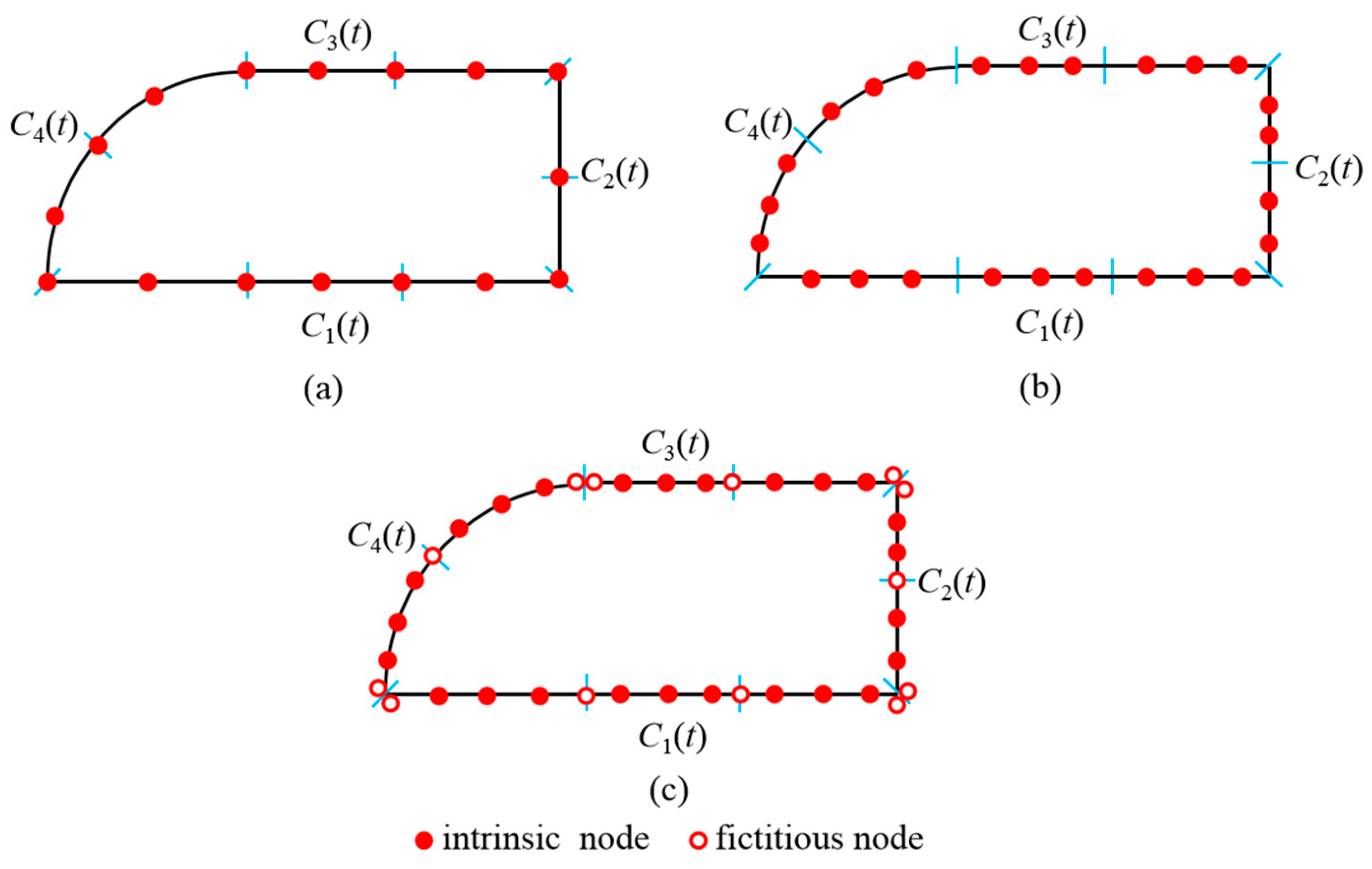
Based on the insight that boundary discretization can be approximated by different types of elements, a novel curve modeling method named dual spline is presented in this paper. As is depicted in Figure 2, the dual spline fitting elements are applied in the implementation of dual spline curve modeling. Combined with fictitious nodes and intrinsic nodes, the accuracy of dual spline fitting elements is superior to conventional elements. The symbols DL1, DL2 and DL3 represent the constant, linear, and quadratic dual spline fitting elements, respectively. The dual spline fitting elements with the notation DL1, DL2 and DL3 indicate the number of interior nodes for the given element. In order to better approximate the continuous and discontinuous curves, two categories of dual spline fitting elements are proposed for curve modeling. As illustrated in Figure 3, the shape functions of DL1, DL2 and DL3 elements used for curve modeling are given by Eqs. (1) ~ (3), respectively.

{\begin{cases} N_{1} = 0.5 ξ (ξ - 1), \\ N_{2} = 0.5 ξ (ξ + 1), \\ N_{3} = (1 + ξ) (1 - ξ), \end{cases}

(1)

{\begin{cases} N_{1} = - \frac{1}{16} (9 ξ^{2} - 1) (ξ - 1), \\ N_{2} = \frac{1}{16} (9 ξ^{2} - 1) (ξ + 1), \\ N_{3} = \frac{9}{16} (ξ^{2} - 1) (3 ξ - 1), \\ N_{4} = - \frac{9}{16} (ξ^{2} - 1) (3 ξ + 1) \end{cases}

(2)

{\begin{cases} N_{1} = \frac{2}{3} ξ (ξ^{2} - \frac{1}{4}) (ξ - 1), \\ N_{2} = \frac{2}{3} ξ (ξ^{2} - \frac{1}{4}) (ξ + 1), \\ N_{3} = - \frac{8}{3} ξ (ξ^{2} - 1) (ξ - \frac{1}{2}), \\ N_{4} = (ξ^{2} - 1) (4 ξ^{2} - 1), \\ N_{5} = - \frac{8}{3} ξ (ξ^{2} - 1) (ξ + \frac{1}{2}) \end{cases}

(3)

where ξ ∈[−1, 1] is the local parameter coordinates in defining shape functions.

2.2. The first-layer interpolation for the dual spline

Dual spline curve modeling is approximated by Lagrange polynomials [24] in the first-layer interpolation. Unlike the conventional interpolation elements, both intrinsic and fictitious nodes of the dual spline must be taken into account. For the dual spline curve modeling, the unknown variables at any point ξ are evaluated by

C (ξ) = \sum_{α = 1}^{n α} N_{α}^{s} (ξ) P (Q_{α}^{s}) + \sum_{β = 1}^{n β} N_{β}^{v} (ξ) P (Q_{β}^{v})

(4)

where

C (ξ)

represents a point defined on the dual spline curve, nα, nβ are the total number of intrinsic nodes and fictitious nodes, respectively;

P (Q_{α}^{s})

N_{α}^{s} (ξ)

indicate the nodal values and shape functions of intrinsic nodes, respectively;

P (Q_{β}^{v})

N_{β}^{v} (ξ)

indicate the nodal values and shape functions of fictitious nodes, respectively.

2.3. The second-layer interpolation for the dual spline

Due to the fictitious nodal values for dual spline curve modeling are not independent, the meshless interpolation technique is developed on the basis of moving least-square (MLS) approximation [25] for interpolating the variables of fictitious nodes in this interpolation. The detail of MLS approximation for second-layer interpolation is described below.

Given a fictitious node

Q_{β}^{v}

, the MLS interpolants in its neighborhood are given by

P (Q_{β}^{v}) = \sum_{i = 1}^{M} Φ_{i}^{s} (t) \hat{P} (Q_{i}^{s})

(5)

For the MLS interpolants of fictitious node

Q_{β}^{v}

, the shape functions

Φ_{i}^{s} (t)

of all intrinsic nodes

Q_{i}^{s}

(i = 1, 2, …, M) are defined as

Φ = {Φ_{1}^{s}, Φ_{2}^{s}, \dots, Φ_{i}^{s}, \dots, Φ_{M}^{s}} = p^{T} (t) A^{- 1} (t) B (t)

(6)

The corresponding vector and matrices are represented by

p^{T} (t) = [1, t, t^{2}, t^{3}], m = 4

(6a)

A^{- 1} (t) = \sum_{i = 1}^{M} w_{i} p (t) p^{T} (t),

(6b)

B (t) = [w_{1} p (t_{1}), w_{2} p (t_{2}), \dots w_{i} p (t_{i}), \dots, w_{M} p (t_{M})]

(6c)

where

w_{i}

(i = 1, 2, …, M) are the weight functions of intrinsic nodes in the neighborhood of the given fictitious node

Q_{β}^{v}

. t represents the parameter values of points on the dual spline curve.

p^{T}

is the basis function vector of relating intrinsic nodes. Note that the fictitious nodal values

\hat{u} (Q_{α}^{s})

are different from the intrinsic nodal values of

u (Q_{α}^{s})

in general. More details of the MLS approximation can be available in [26,27].

3. Adaptive curve construction using dual spline

The dual spline curve modeling method takes well-known steps by preprocessing the initial points, dominant point selection, and fair dual spline construction. However, the uniqueness of the proposed approach lies in dominant point selection and fair dual spline construction for smooth curve modeling.

3.1. Preprocessing of points for curve modeling

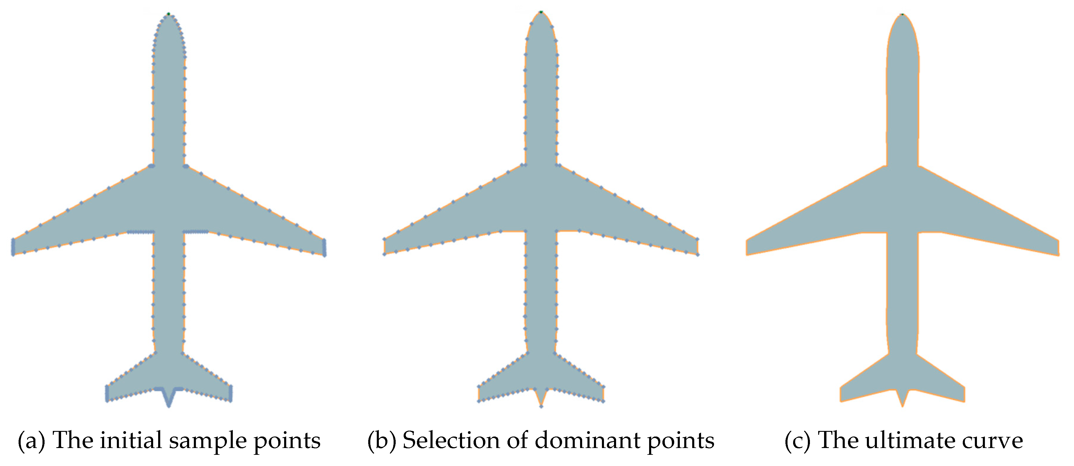
In order to create a high-quality and well-shaped dual spline curve, it is very essential that the measured points should be pre-processed before curve modeling. Dual spline curve modeling is implemented by adaptive curve refinement using dominant points. The dominant points for curve modeling are extracted by considering the geometry definition, the position, and the curvature of each measured point, such as inflection points and local curvature maximum (LCM) points [28]. Each of these feature points works better under particular circumstances, and due care needs to be taken in deciding which kind of dominant points for selection. However, there are some undesired noisy points in the implementation of preprocessing of points for curve modeling. If the dominant points are selected without considering any geometrical features, dual spline curve modeling will cause a lack of smoothness in the ultimate curve representation.

In the preprocessing procedure of dual spline curve modeling, two types of dominant points are considered, namely, the LCM points and the endpoints. Compared to the others, the curvature characteristics of LCM points are capable of providing more valuable information about the main features of the given points. For the given curve

C (t)

, a mathematical description of the curvature

k_{i}

at each point

P_{i}

is defined by

k_{i} = ‖ \dot{C} ({\bar{t}}_{i}) \times \ddot{C} ({\bar{t}}_{i}) ‖ / {‖ \dot{C} ({\bar{t}}_{i}) ‖}^{3}

(7)

where

\dot{C} ({\bar{t}}_{i})

and

\ddot{C} ({\bar{t}}_{i})

are the first and second derivatives of the curve

C (t)

at the parameter

{\bar{t}}_{i}

, respectively.

According to the curvatures

k_{i}

estimated at the point set, the point

P_{i}

is taken for an LCM point based on the following rules, i.e.,

k_{i} > k_{i - 1}

and

k_{i} > k_{i - 1}

. The lower curvature bound

k_{l o w}

for selection of dominant points can be defined as

k_{l o w} = k_{a v g} / 4

, where

k_{a v g}

is the average of all the discrete point set. Most of the LCM points with curvatures less than

k_{l o w}

are excluded in the optimal dominant points. In addition, the distinct discontinuous points of piecewise parametric curves are required to be separated independently for further processing. Two end points are also very essential for high-quality curve modeling.

With the dominant points for curve modeling available, a well-shaped dual spline curve can be formed based on the adaptive refinement scheme. As is shown in Figure 4, The results demonstrate the advantages of not only fewer nodes and simple formulation, but also feasible implementation and satisfactory accuracy. It is appealing that a well-shaped curve can be achieved by dominant points selection for capturing geometric features.

3.2. Dual spline for smooth curve modeling

Given a collection of points measured from the geometric model, the requirements of the fitting principle must be satisfied. Specifically, the scattered point set is required to be arranged in sequence and presented in dual spline form. In the implementation of curve modeling, dual spline fairing techniques are adopted here for the parameterization of the given points, aiming to approximate these points to form a smooth curve. Significant warp and undesired twists are entirely preventable through a dual spline curve fairing procedure.

With the given ordered dominant points, a dual spline curve can be constructed by determining the exact interpolation of certain parameter values with piecewise dual spline fitting elements. For dual spline curve modeling, the shaped functions are determined by the parameterized pattern of discrete point set. Without loss of generality, assume that dominant points

P_{i} (i = 0, 1, 2, \dots, n)

are selected among the given point set, the mathematical description of the dual spline curve is defined by

C (t) = \sum_{i = 0}^{n} N_{i, p} (t) P_{i} (t_{\min} \leq t \leq t_{\max})

(8)

where

N_{i, p} (t)

are the shape functions of intrinsic nodes or fictitious nodes defined on the parameter space

T = {t_{\min}, t_{1}, \dots, t_{i}, \dots, t_{\max}}

. The parameter vector

T

consists of non-decreasing real-valued knots, which is determined by the chord length method.

Note that the parameterization for dual spline curve modeling is determined by the distributing form of the given scattered points. In order to create a well-shaped dual spline curve, the point filtering procedure is incorporated to displace the undesired noisy points. With the point filtering procedure, the parameter value

t_{i}

for each dominant point can be computed by the following form

t_{i} = \frac{\sum_{j = 1}^{i} {| Q_{j} - Q_{j - 1} |}^{\frac{1}{2}}}{\sum_{j = 1}^{n} {| Q_{j} - Q_{j - 1} |}^{\frac{1}{2}}}

(9)

In the process of dual spline curve modeling, the dual spline fitting elements are constructed in the ordered parameter space. For each dual interpolation element, the parameter values

t_{i}

can also be represented in terms of the intrinsic nodal coordinates in defining shape functions. Consequently, adaptive dual spline curve construction with less deviation can be achieved for arbitrary discrete point sets.

4. Approximation of continuous and discontinuous curve representation

Due to the advantages of dual spline fitting elements in terms of accuracy and performance, dual splines are flexible and convenient to approximate the arbitrary curve representation. By adding fictitious nodes and intrinsic nodes inside or at vertices of elements, the proposed approach is flexible and convenient to approximate continuous or discontinuous curve representation by using dual spline. In addition, we also demonstrate the potential advantages of dual spline for alleviating the heavy task of complex geometry repair.

Combined with Lagrange interpolation polynomial and meshless method, the proposed approach is capable to approximate continuous or discontinuous curves along the non-smooth boundary.

4.1. Dual spline for continuous curve representation

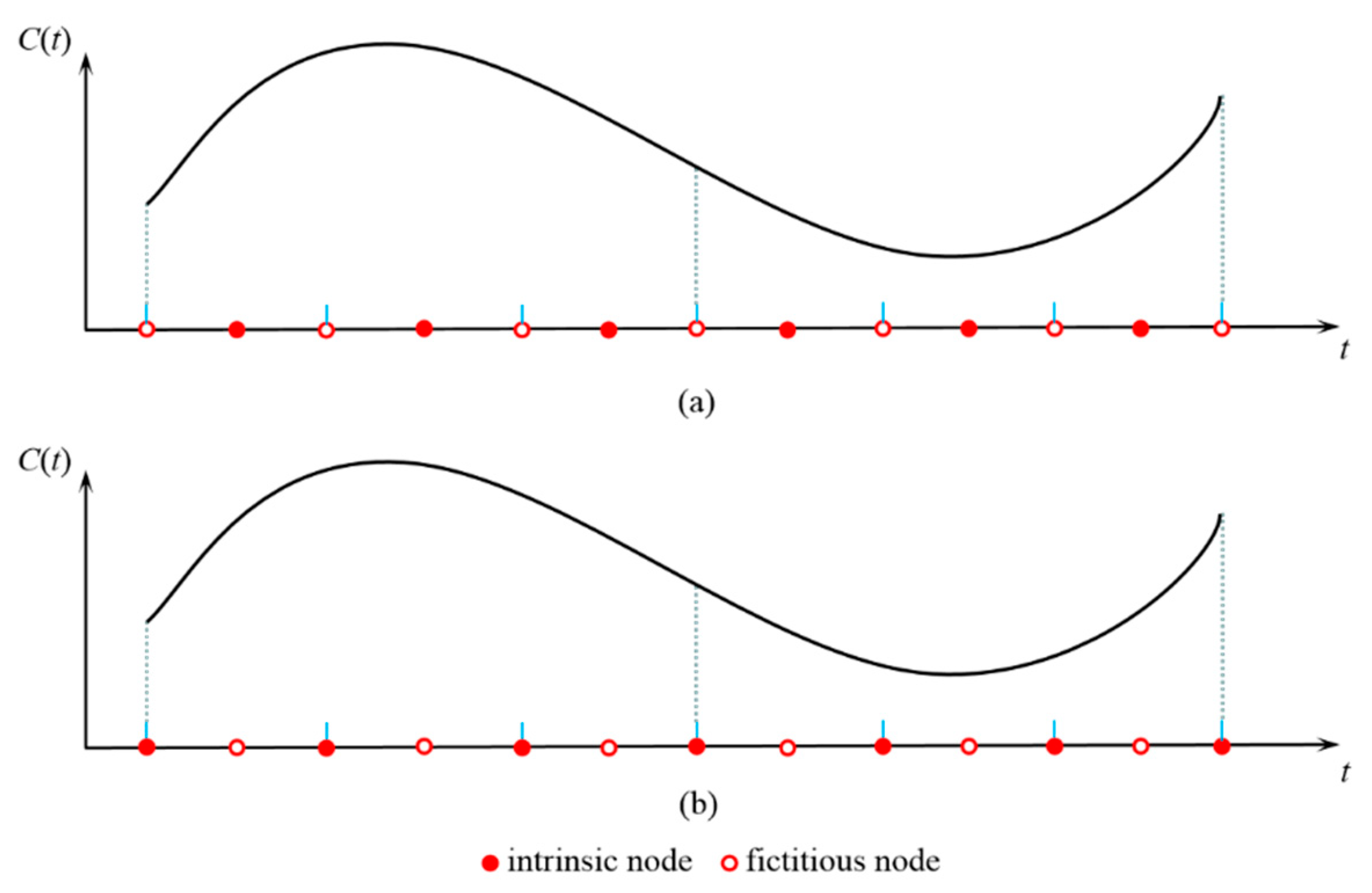
The parametric representations of geometric curves are generally classified into two primary kinds: continuous functions and discontinuous functions. In contrast to conventional methods, the dual spline curve modeling method can naturally approximate both continuous and discontinuous functions based on the introduction of fictitious nodes. Figure 5 provides a schematic illustration of a dual spline for continuous curve representation.

For the continuous curve representation, arbitrary types of dual spline fitting elements can approximate continuous curves. As shown in Figure 5, intrinsic or fictitious nodes can be distributed on the boundary of the elements. In this case, the dual spline fitting elements are equivalent to conventional interpolation elements. By adding fictitious and intrinsic nodes inside or at the vertices of elements, the dual spline is flexible and adaptable to approximate the continuous curve.

4.2. Dual spline for discontinuous curve representation

In geometric modeling, curve fitting in computer graphics prefers piecewise parametric curves to represent geometric entities. The ultimate goal of curve modeling is to construct a fair freeform curve with specific geometric properties. However, due to the complexity of solid modeling, there are some unwanted geometric features, such as short edges, narrow faces, fragmentary boundary edges, sharp features, etc. In addition, another long-standing issue of the unavoidable gaps that arise when representing the trimming curves of intersection among arbitrary parametric surfaces. Consequently, the geometric models are not mathematically watertight using Boolean operations. That is, gaps are unavoidable in conventional trimmed mathematical models. For complex geometries, accurate approximation of parametric trimming curves with discontinuous functions is still a bottleneck in curve modeling.

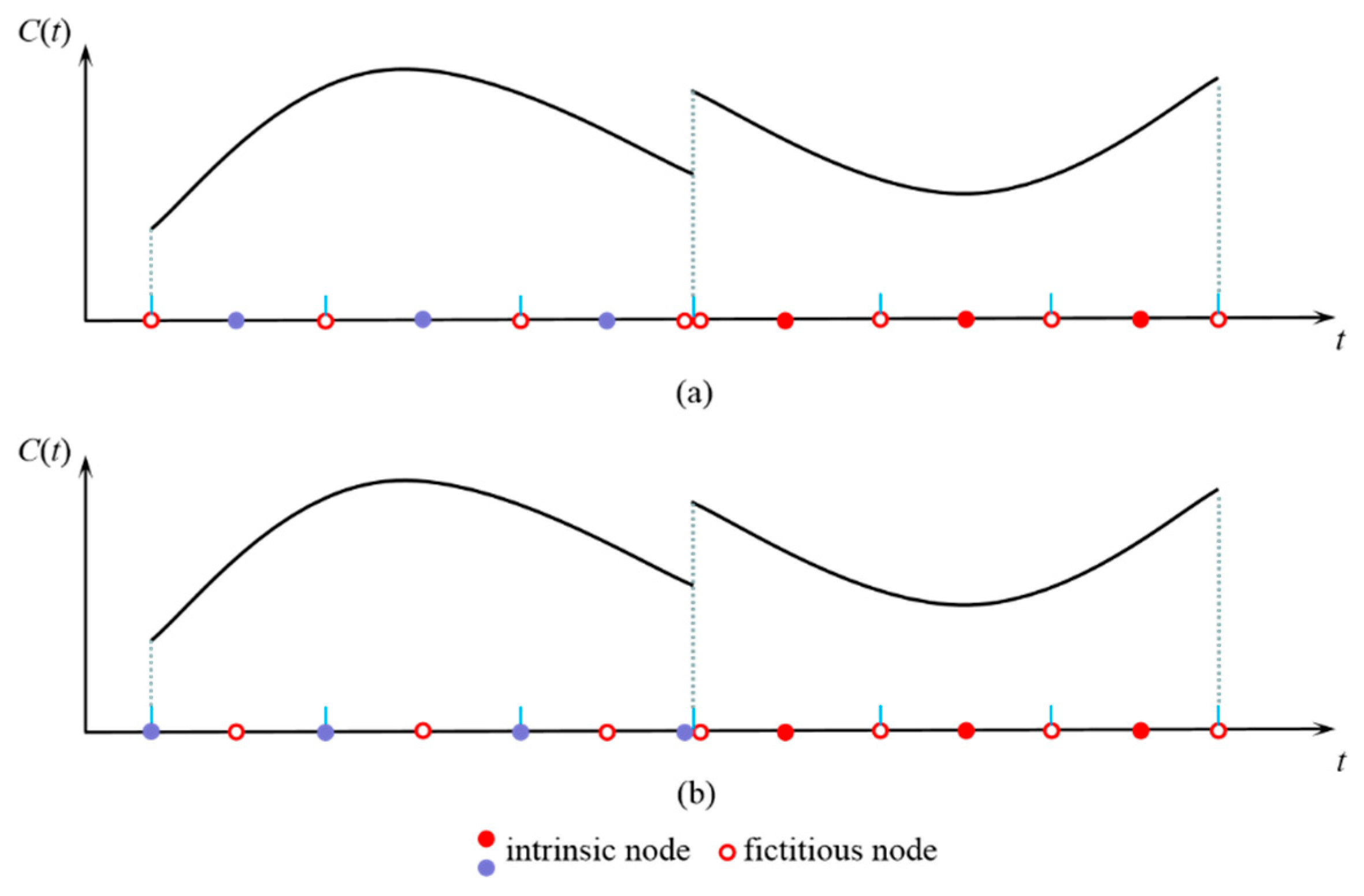
For the discontinuous curve representation or geometry defeaturing, multiple nodes are assigned separately on the non-smooth geometric boundary. In general, fictitious and intrinsic nodes can be distributed on the boundary of the elements reasonably. As depicted in Figure 6, the fictitious nodes on the discontinuous boundary are generated at identical locations separately. These fictitious nodes are situated at endpoints of two adjacent curves, which makes dual spline naturally independent for discontinuous curve modeling. Unlike continuous curve representation using dual spline, the fictitious nodes at endpoints are opaque when determining the influence domain in MLS. That is, the intrinsic nodes lying on the adjacent curves are not included in the search range. Based on flexible configuration features and stable performance, the dilemma of complex geometry repair using dual spline is also avoidable.

5. Experimental results

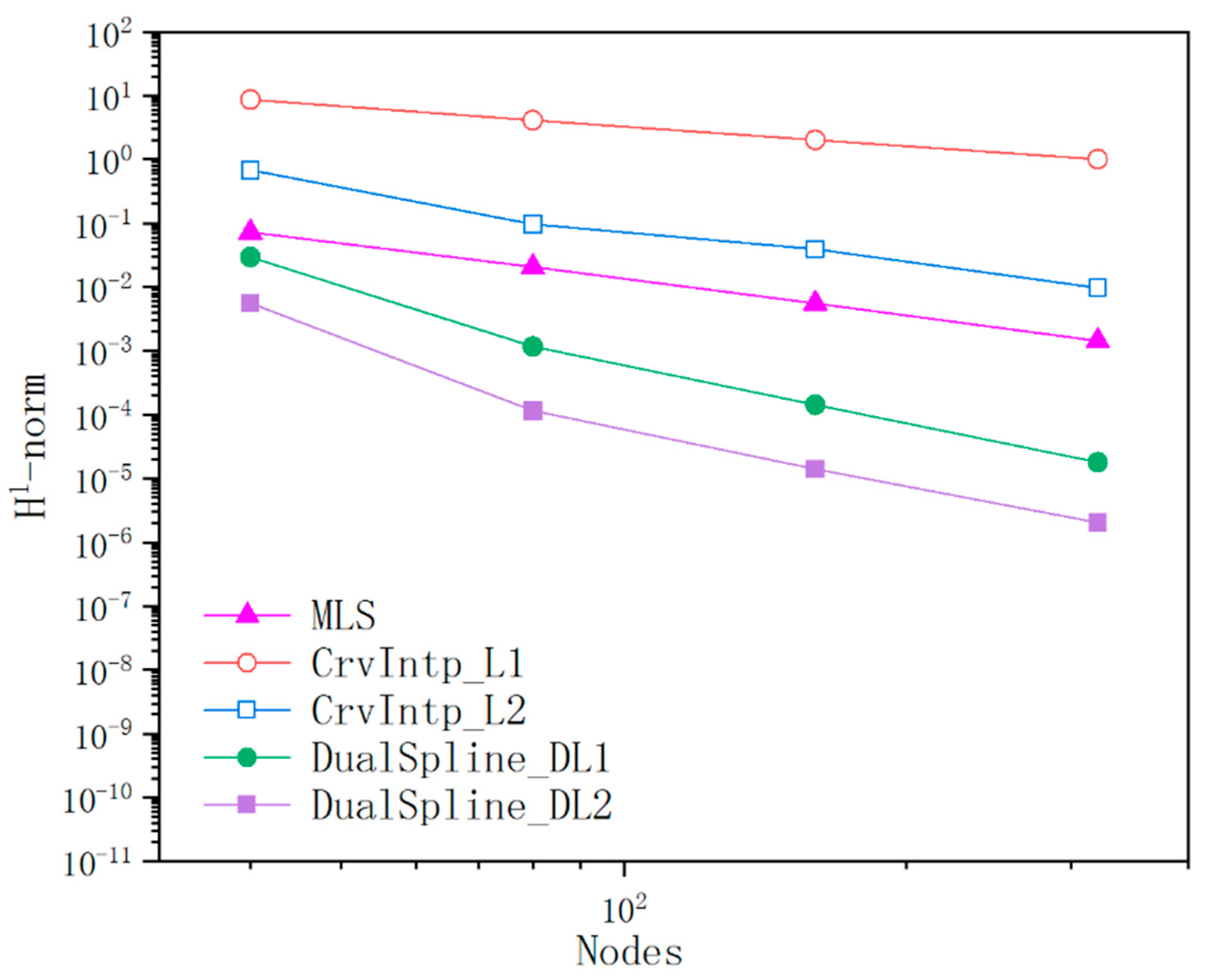
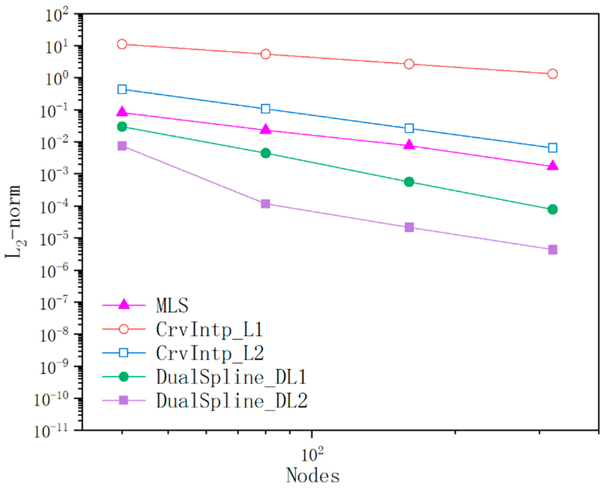
The accuracy and feasibility of the proposed method are verified through several numerical examples calculated by dual spline. A comparison of the dual spline and conventional approaches for curve modeling is also given in this section. The results of numerical examples show that the accuracy and convergence are satisfactory, and it will be helpful to for practical purposes. Several examples of different types of dual spline fitting elements are employed to verify the availability that the dual spline is reasonable and applicable to approximate the continuous and discontinuous curve modeling in Section 5.2 and Section 5.3, respectively. According to the proposed method, relative errors measured in H1-norm and L2-norm [29,30] are given to demonstrate the accuracy and convergence of dual spline, which are defined as

H^{1} - n o r m : e r r o r = \frac{1}{N} \sum_{i = 1}^{N} | P_{i}^{(e)} - P_{i}^{(n)} |

(10)

L_{2} - n o r m : e r r o r = \sqrt{\frac{1}{N} \sum_{i = 1}^{N} {| P_{i}^{(e)} - P_{i}^{(n)} |}^{2}}

(11)

where N indicates the number of the specific sample points for measurement,

P_{i}^{(e)}

and

P_{i}^{(n)}

represent the reference points and new generated points, respectively.

5.1. Convergence assessment of dual spline curve modeling

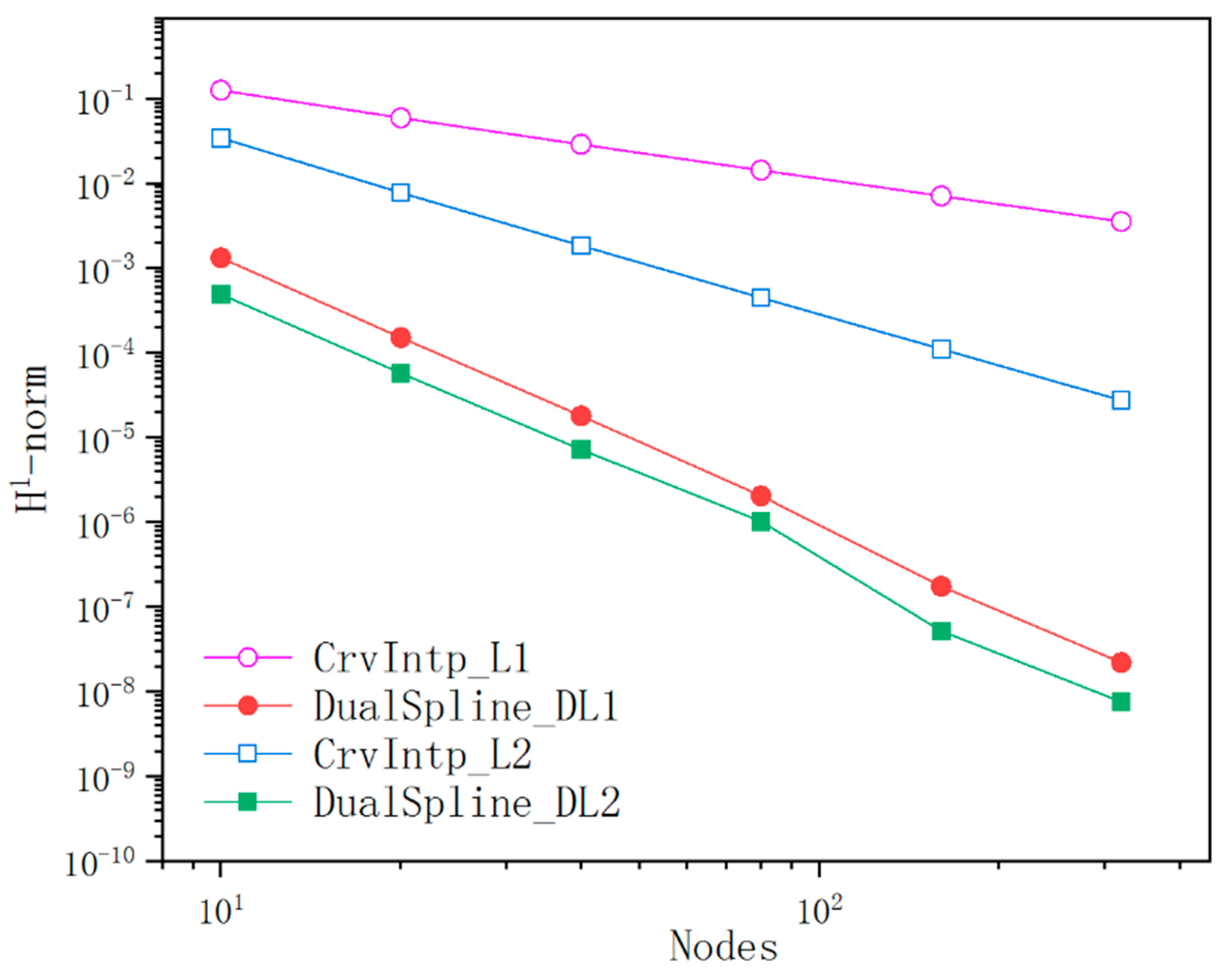
This paper presents the dual spline curve modeling method for continuous and discontinuous curve representation from arbitrary discrete point sets. The first example is done to verify the effectiveness and convergence behavior of the proposed method. Unless otherwise mentioned, the constant, linear, and quadratic elements in dual spline curve modeling are denoted by DualSpline_DL1, DualSpline_ DL2, and DualSpline_DL3, respectively. The conventional elements with the notation CrvIntp_L1, CrvIntp_L2, and CrvIntp_L3 represent constant, linear, and quadratic interpolation elements, respectively. To illustrate the accuracy and convergence of the curve modeling method, a set of random points are sampled from the following arbitrary plane curve, which is given by

C (t) = 0 . 0912 t^{3} - 0 . 8596 t^{2} + 1 . 8527 t - 0 . 1649

(12)

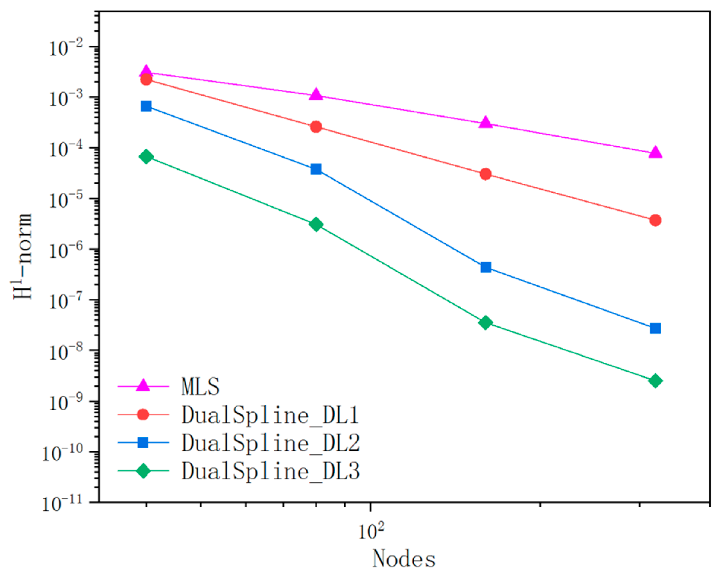
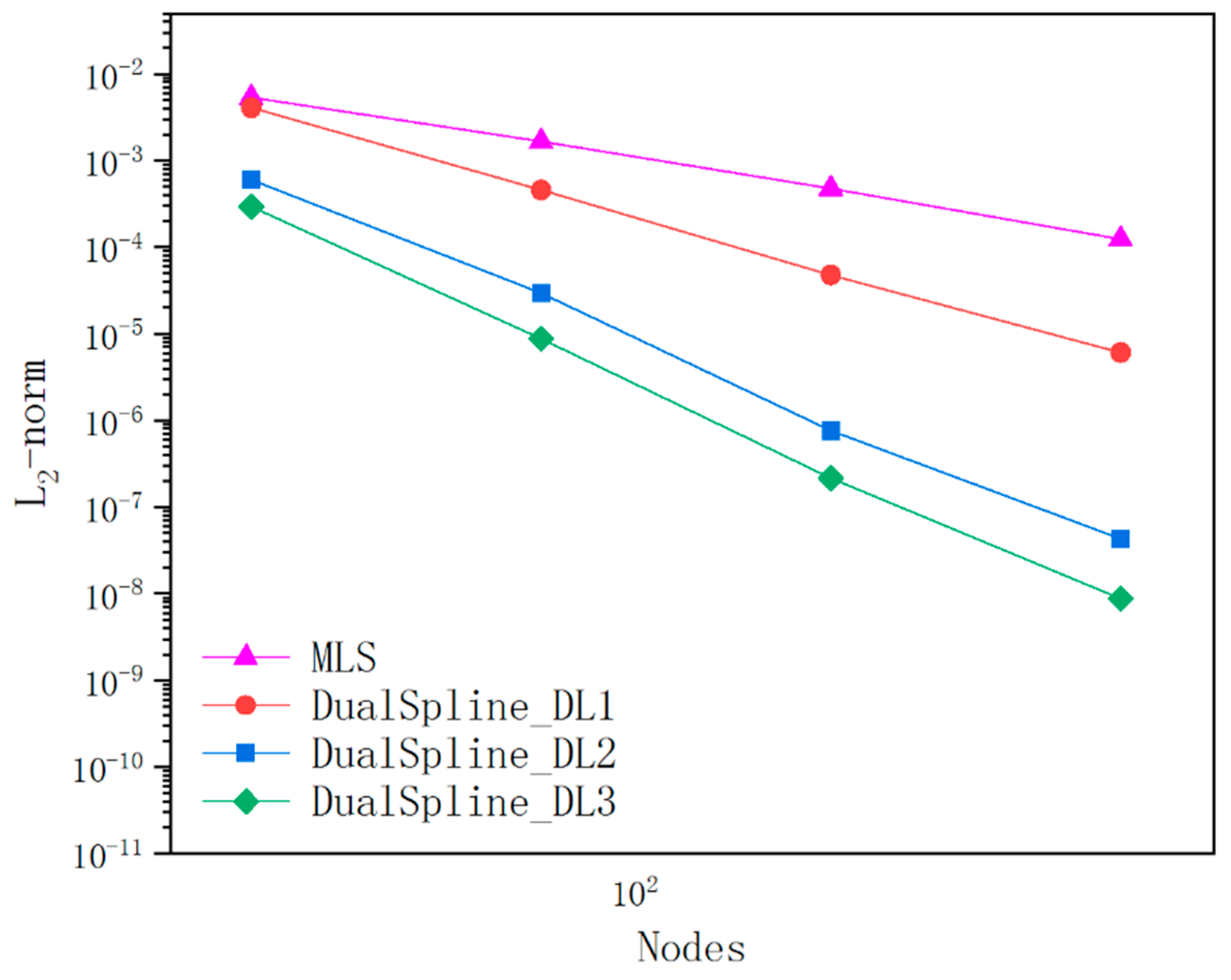
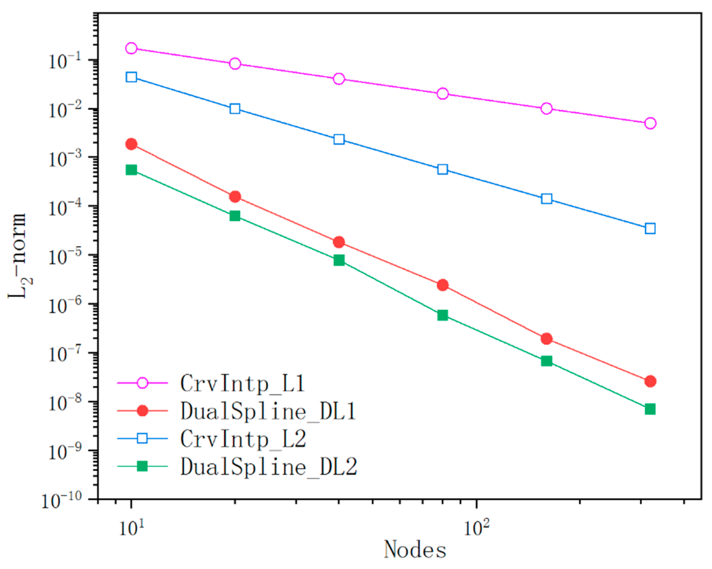
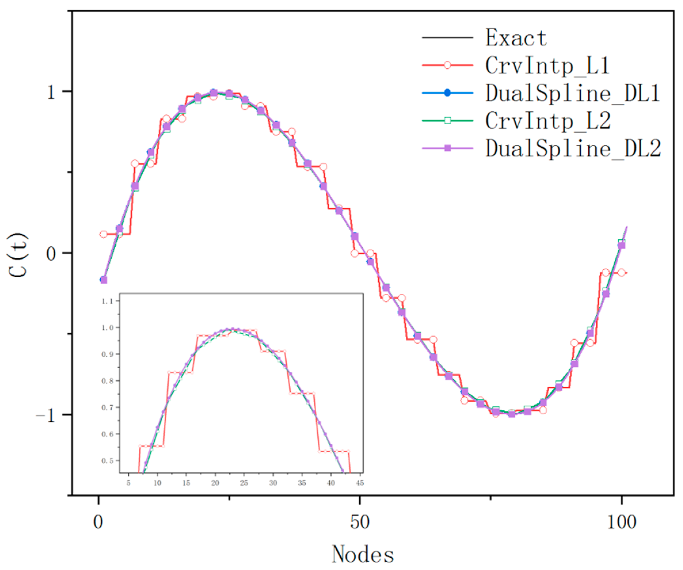
The given geometric curve is subdivided into 10, 20, 40, 80, 160, and 320 dual spline fitting elements to study the convergence behavior of different orders of elements, respectively. The interpolation points are uniformly distributed on the given curve. Comparison of the convergence performance of the dual spline curve modeling with different order of elements are shown in Figure 7 and Figure 8. Results of the ultimate curve modeling using dual spline and conventional interpolation methods with 40 elements are shown in Figure 9, respectively. According to the experimental results, the accuracy and convergence of dual spline are both superior to the conventional interpolation methods under the same number of elements. It is also appealing that the dual spline curve modeling method is more flexible and better at converging with increasing nodes.

5.2. Evaluation of dual spline for arbitrary curve modeling

The second example further demonstrates the feasibility and availability of dual spline for arbitrary curve modeling. The chord length method distributes the interpolation points on the given curve according to the geometric features. In order to construct a dual spline curve with high quality, the point filtering procedure is implemented to preprocess the undesired noisy points. Different types of dual spline fitting elements are incorporated into the implementation of dual spline, which is adopted to examine the effectiveness and convergence behavior of dual spline curve modeling with different parameterizations.

C (t) = 2 e^{- 0.5 t} \sin (2 π t)

(13)

Figure 10. Comparison of accuracy between dual spline and MLS(H¹-norm).

Figure 11. Comparison of accuracy between dual spline and MLS(L₂-norm).

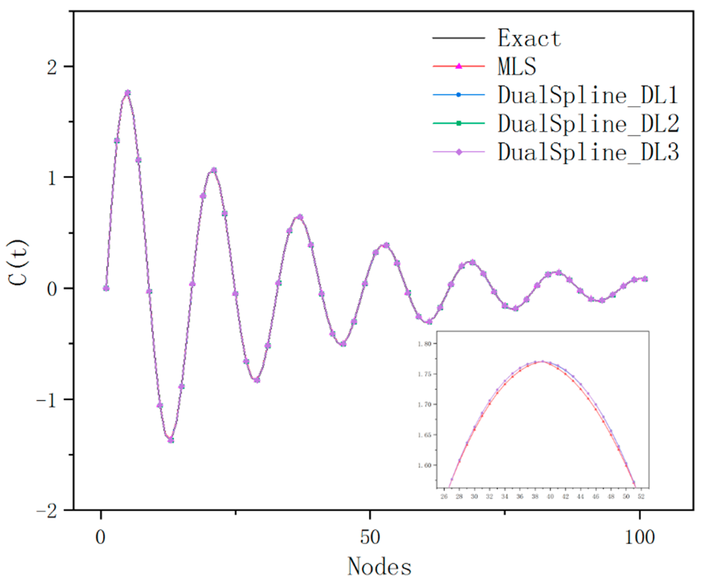
In the case that tolerance is specified, we implemented the dual spline for arbitrary curve modeling with a total of 40, 80, 160, and 320 dual spline fitting elements, respectively. Different parameterization does not influence the ultimate dual spline curve modeling. It also verified that the dual spline curve modeling is less sensitive to the density and distribution of the elements. The curve modeling results of the dual spline with a total of 80 different types of dual spline fitting elements and MLS approximation are respectively shown in Figure 12. 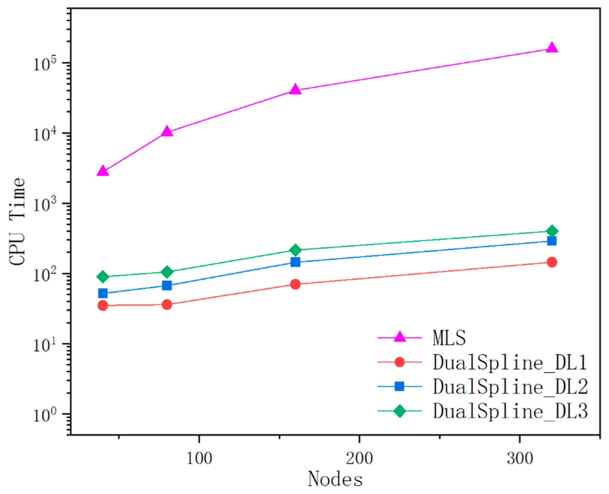As is illustrated in Figure 13, the dual spline can main the interpolation accuracy and improve the calculation efficiency in comparison with the MLS. The curve modeling results of dual spline and MLS are evaluated from 1000 measuring points uniformly distributed in parameter space. The CPU time involves the interpolation construction of dual spline and the time-consuming process of MLS matrix inversion. It is appealing that the dual spline with few interpolation nodes can obtain higher accuracy and efficiency than the MLS approximation.

5.3. Evaluation of dual spline for curve modeling with non-smooth junctions

For the curve representation with non-smooth junctions, the value of predicted curve expression changes precipitously in the vicinity of the discontinuous point or non-smooth geometric boundary. It is tricky to simultaneously approximate the continuous or discontinuous curve by using conventional methods. By adding fictitious and intrinsic nodes in the interpolation elements, the dual spline is also a unique and efficient technique for curve modeling with non-smooth geometric boundary. To further examine the behavior of dual spline curve modeling, arbitrary curve modeling with non-smooth junctions is investigated. The specific representation of discontinuous curve modeling is given by

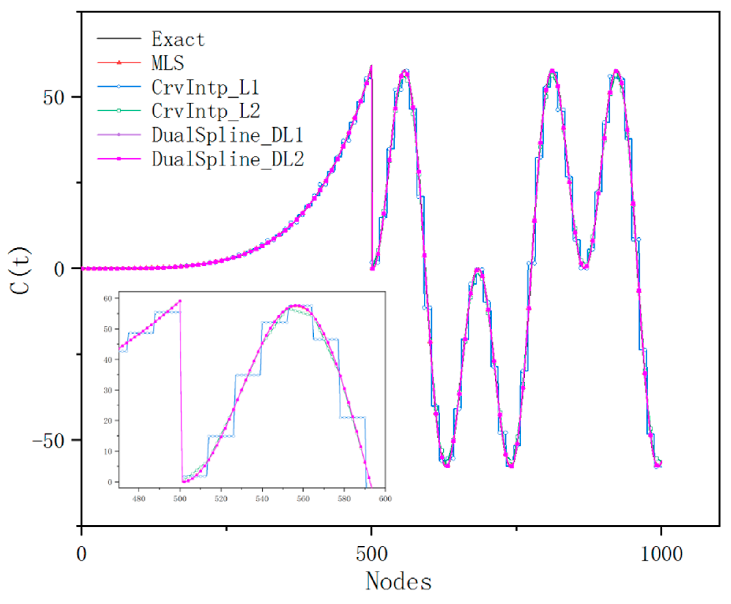
C (t) = {\begin{cases} e^{t} t^{3} t \in [0, 2], \\ 300 \sin (t) \sin (2 t) \cos (t) \cos (2 t) t \in (2, 2 π] \end{cases}

(14)

This example is given to discuss the reliability, stability, and convergence behavior of dual spline compared with other conventional methods. The dual spline is implemented by 40, 80, 160, and 320 elements to study the convergence performance, respectively. For a fair comparison, the conventional interpolation methods and MLS approximation are implemented by searching the smooth range of the piecewise function. When determining the influence domain in MLS approximation, the discontinuous point is deemed as the opaque node; that is, the reference nodes beyond the discontinuous point are not included. As illustrated in Figure 14 and Figure 15, high flexibility and superior performance can be affirmative in the implementation of the dual spline. As is depicted in Figure 16, since the connectivity requirements of conventional curve modeling methods, only the single value for each node can be obtained by MLS or traditional interpolation techniques, which is incapable of approximating the discontinuous region. Due to the existence of multiple nodes at the discontinuous boundary, discontinuous curve representation can be naturally approximated by dual spline.

5.4. Evaluation of dual spline for geometry defeaturing

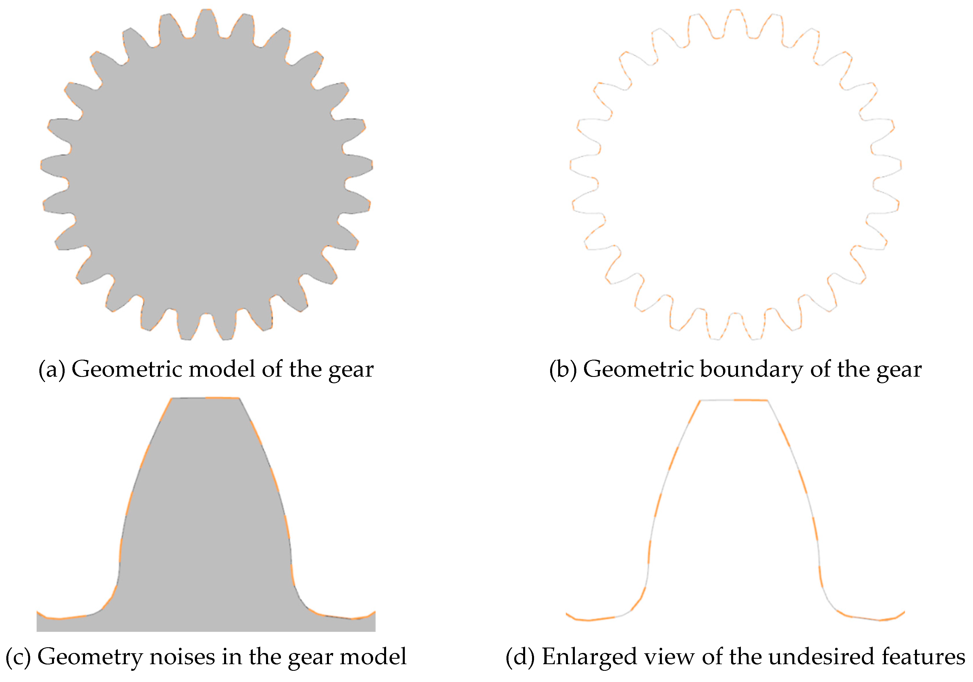
The primary goal of curve modeling is to construct a fair free-form curve with certain geometric properties. Due to the trimmed curves are not mathematically watertight because of some unwanted gaps or holes, some disgusting geometric features are often unavoidable in solid modeling. However, conventional curve modeling methods cannot fulfill their primary role of naturally representing the discontinuous curve with non-smooth junctions. Complicated and diversified curve folds are observed in smooth skinning when using high-order curves for geometry repair. For complex geometries, automatic geometry repair and mesh generation is still a bottleneck in CAE analysis. A complicated curve fitting with undesired features shown in Figure 17 is investigated to study the performance of the dual spline representation for complex geometries.

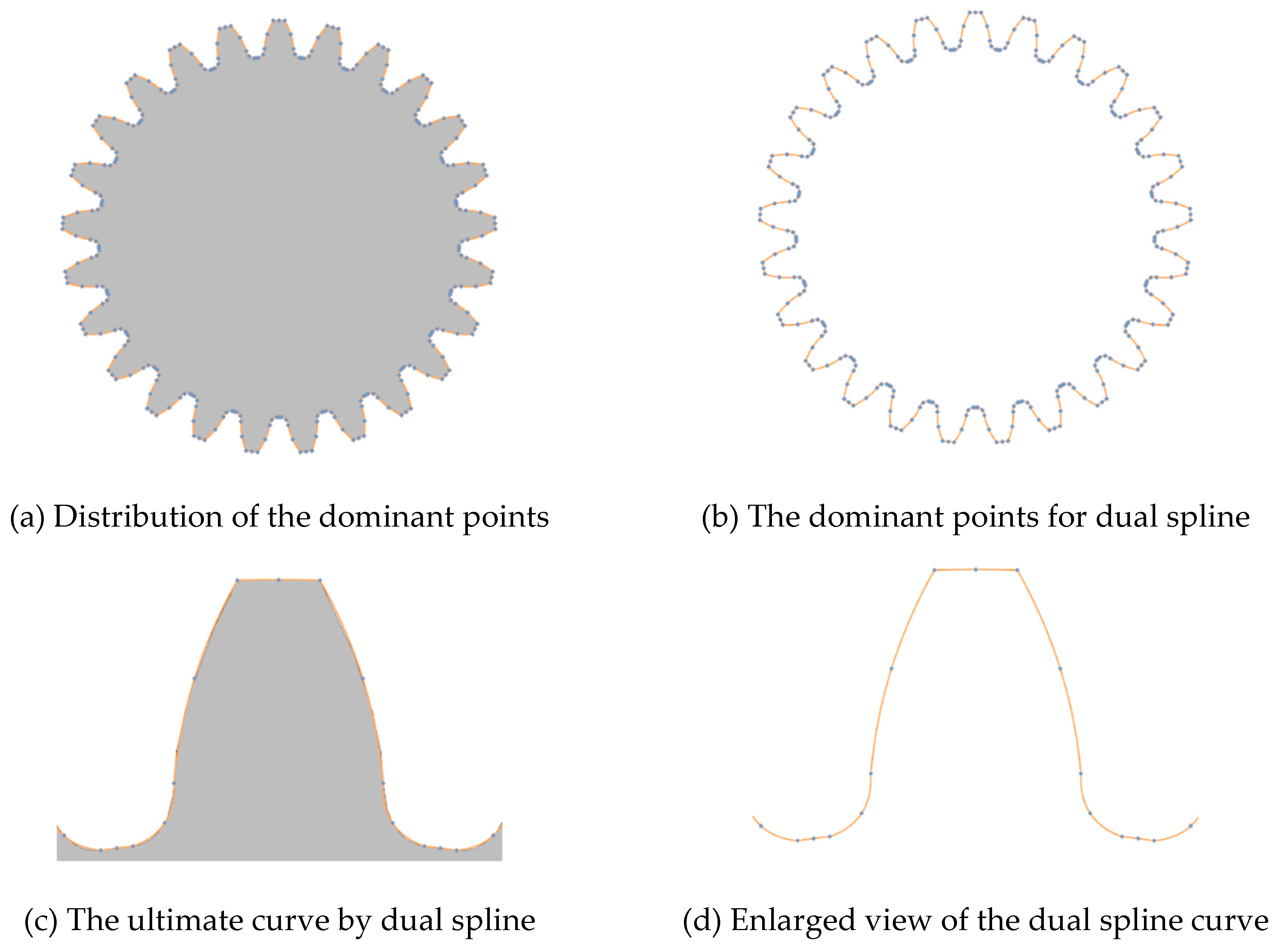
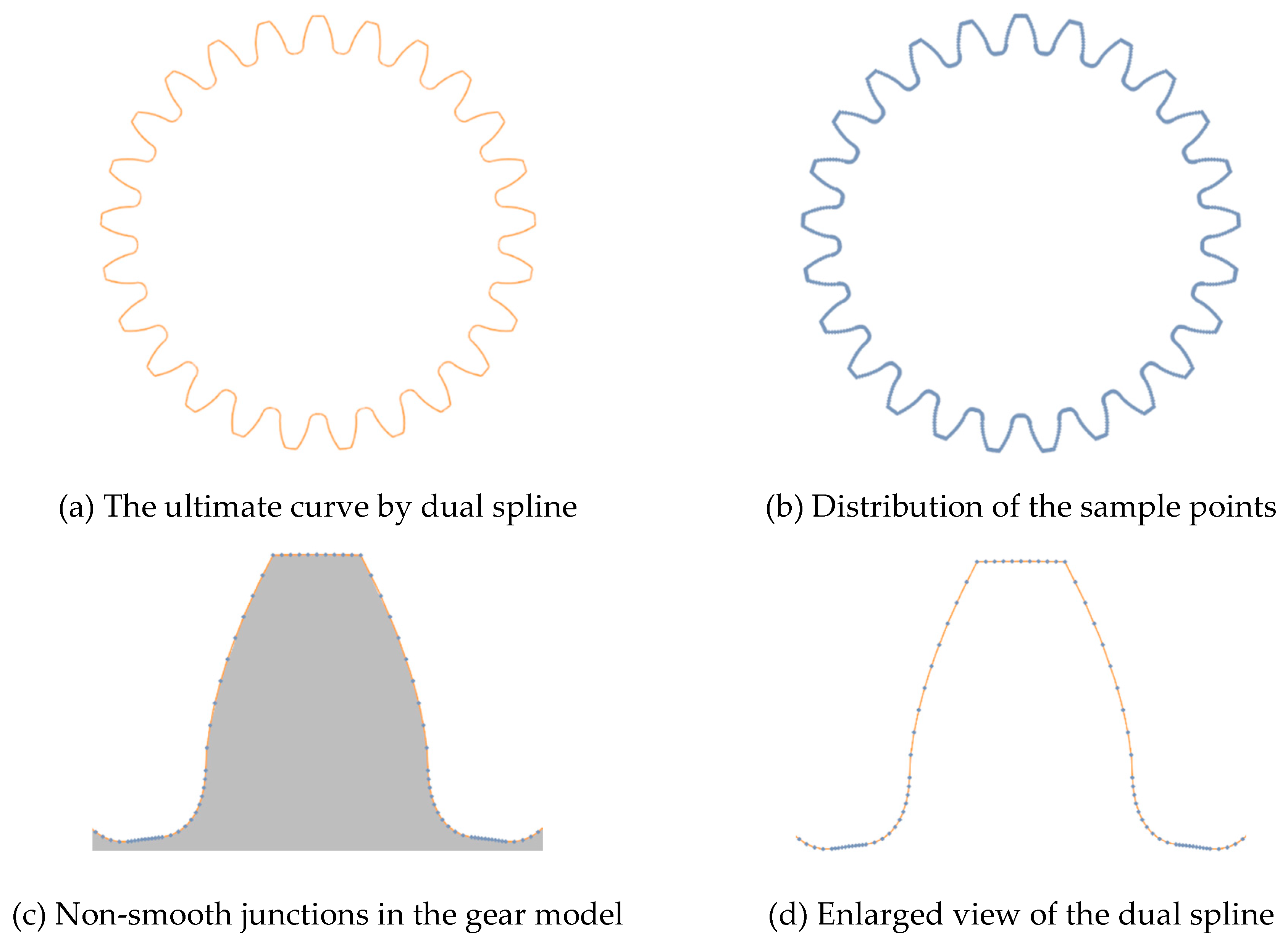
This example demonstrates the potential advantages of dual spline to deal with complex geometry models in a fully automated manner. The real-world geometries of the gear was downloaded from the web without any feature removal or alteration. The outer contour of the gear model is comprised of a few short edges, which brings some problems in mesh generation and further analysis. An entire dual spline curve is constructed around the boundary of the gear based on the adaptive curve refinement technique.

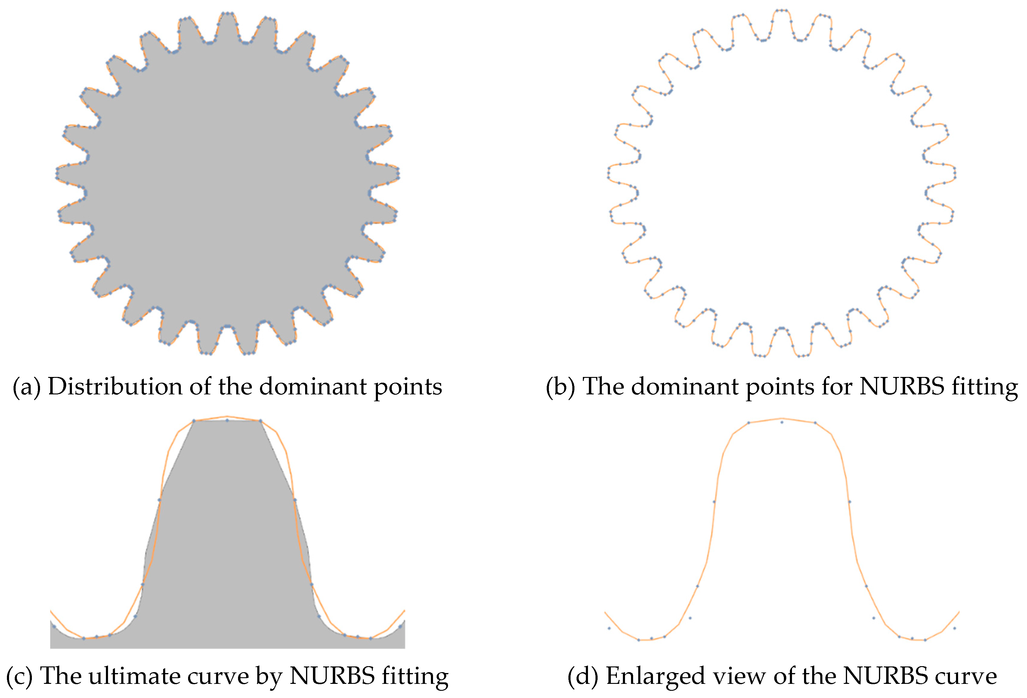
A comparison of convergence and accuracy of the dual spline and NURBS curve fitting method for geometry defeaturing is presented in Figure 18 and Figure 19. It is undeniable that NURBS is the excellent representative form and the internationally recognized standard for curve and surface, which finds wide application in three-dimensional modeling. It is evident from Figure 19 that the NURBS curve cannot well handle the complex geometry models with non-smooth junctions when a higher-degree curve fitting process is performed. Since multiple fictitious nodes are assigned on the sharp corners, the dual spline can be well approximated by the boundary of the gear model, which is a potential advantage of the proposed method for complex geometry repair and automatic mesh generation.

6. Conclusions

This paper presents an adaptive dual spline curve modeling method for continuous or discontinuous curve representation. The dual spline has some prominent geometric properties over other methods, such as improvement of the interpolation accuracy, the unity of Lagrange polynomial and meshless interpolation, and alleviation of the continuity requirements of curve fitting. In the implementation of dual spline, a novel type of element named dual spline fitting elements are introduced for curve modeling. Combined with intrinsic nodes and fictitious nodes, the proposed approach is flexible and convenient to approximate continuous or discontinuous curve representation by using dual spline. Even with some irregular elements in curve modeling, the dual spline can exhibit higher flexibility and superior performance.

Experimental results illustrate the validity, efficiency, and feasibility of the dual spline curve modeling method. Besides, we also demonstrate the potential advantages of dual spline for alleviating the heavy task of complex geometry repair. By distributing the fictitious nodes and intrinsic nodes at the non-smooth geometric boundary, the dual spline is also an efficient and flexible technique for complex geometry repair. The results demonstrate the advantages of fewer nodes and simple formulation, satisfactory accuracy, and better convergence. More complex geometry repair and isogeometric analysis for arbitrary structures can be observed by the 3-D dual spline surface fitting in future work.

Acknowledgements

This work was supported by the National Natural Science Foundation of China (12202251, 12172201, 51805299), China Postdoctoral Science Foundation Project (2021M702024, 2022M712393), Ministry of Education Industry-school Cooperative Education Project(220606517023742), the Key Research and Development Project of Shandong Province (2019GGX104081, 2019GGX104033), Zibo City School-City Integration Project (2018ZBXC265), the Shandong Provincial Natural Science Foundation, China (ZR2022ME122, ZR2022QA072), the Scientific Research Project of Shandong University of Technology (4041/420047, 4003/122237, 9101/2222431), Shandong Province’s Key Support Regions Introducing Urgently Needed Talent Projects, and Young Innovative Talents Introduction and Training Program Project of Shandong Provincial Department of Education.

References

Albdairy, A.M.; Al-Duroobi, A.A.; Tawfiq, M.A. Pre-Processing and Surface Reconstruction of Points Cloud Based on Chord Angle Algorithm Technique. Al-Khwarizmi Eng. J. 2020, 16, 34–42. [Google Scholar] [CrossRef]
Huang, M.C.; Tai, C.C. The pre-processing of data points for curve fitting in reverse engineering. Int. J. Adv. Manuf. Technol. 2000, 16, 635–642. [Google Scholar] [CrossRef]
Yang, X. Curve fitting and fairing using conic splines. Comput.-Aided Des. 2004, 36, 461–472. [Google Scholar] [CrossRef]
Yamaguchi, F. Curves and Surfaces in Computer Aided Geometric Design; Springer Science & Business Media: Berlin/Heidelberg, Germany, 2012. [Google Scholar]
Huang, J.; Chen, L.; Izumiya, S.; Pei, D. Geometry of special curves and surfaces in 3-space form. J. Geom. Phys. 2019, 136, 31–38. [Google Scholar] [CrossRef]
Hughes TJ, R.; Cottrell, J.A.; Bazilevs, Y. Isogeometric analysis: CAD, finite elements, NURBS, exact geometry and mesh refinement. Comput. Methods Appl. Mech. Eng. 2005, 194, 4135–4195. [Google Scholar] [CrossRef]
Kosinka, J.; Cashman, T.J. Watertight conversion of trimmed CAD surfaces to Clough–Tocher splines. Comput. Aided Geom. Des. 2015, 37, 25–41. [Google Scholar] [CrossRef]
Mohan, S.; Kweon, S.H.; Lee, D.M.; Yang, S.H. Parametric NURBS curve interpolators: A review. Int. J. Precis. Eng. Manuf. 2008, 9, 84–92. [Google Scholar]
Mirzaee, F.; Alipour, S. Cubic B-spline approximation for linear stochastic integro-differential equation of fractional order. J. Comput. Appl. Math. 2020, 366, 112440. [Google Scholar] [CrossRef]
Sederberg, T.W.; Zheng, J.; Bakenov, A.; Nasri, A. T-splines and T-NURCCs. ACM Trans. Graph. (TOG) 2003, 22, 477–484. [Google Scholar] [CrossRef]
Smarzewski, R.; Bujalska, A. Uniform convergence of cubic and quadratic X-spline interpolants. IMA J. Numer. Anal. 1983, 3, 353–372. [Google Scholar] [CrossRef]
Knez, M.; Pelosi, F.; Sampoli, M.L. Spline surfaces with C1 quintic PH isoparametric curves. Comput. Aided Geom. Des. 2020, 79, 101839. [Google Scholar] [CrossRef]
Yang, L.; Zeng, X.M. Bézier curves and surfaces with shape parameters. Int. J. Comput. Math. 2009, 86, 1253–1263. [Google Scholar] [CrossRef]
Sederberg, T.W.; Finnigan, G.T.; Li, X.; Lin, H.; Ipson, H. Watertight trimmed NURBS. ACM Trans. Graph. (TOG) 2008, 27, 1–8. [Google Scholar] [CrossRef]
Li, X.; Chang, Y. Non-uniform interpolatory subdivision surface. Appl. Math. Comput. 2018, 324, 239–253. [Google Scholar] [CrossRef]
Chen, L.; Lu, C.; Zhao, W.; Chen, H.; Zheng, C. Subdivision surfaces—Boundary element accelerated by fast multipole for the structural acoustic problem. J. Theor. Comput. Acoust. 2020, 28, 2050011. [Google Scholar] [CrossRef]
Zhang, B.; Zheng, H.; Song, W. A non-stationary Catmull–Clark subdivision scheme with shape control. Graph. Models 2019, 106, 101046. [Google Scholar] [CrossRef]
Alam, M.N.; Li, X. Non-uniform Doo-Sabin subdivision surface via eigen polygon. J. Syst. Sci. Complex. 2021, 34, 3–20. [Google Scholar] [CrossRef]
Cheng FH, F.; Fan, F.T.; Lai, S.H.; Huang, C.L.; Wang, J.X.; Yong, J.H. Loop subdivision surface based progressive interpolation. J. Comput. Sci. Technol. 2009, 24, 39–46. [Google Scholar] [CrossRef]
Zhang, J.; Chi, B.T.; Singh, K.M.; Zhong, Y.; Ju, C. A binary-tree element subdivision method for evaluation of nearly singular domain integrals with continuous or discontinuous kernel. J. Comput. Appl. Math. 2019, 362, 22–40. [Google Scholar] [CrossRef]
Zhang, J.; Chi, B.T.; Singh, K.M.; Zhong, Y.; Ju, C. A binary-tree element subdivision method for evaluation of singular domain integrals with continuous or discontinuous kernel. Eng. Anal. Bound. Elem. 2020, 116, 14–30. [Google Scholar] [CrossRef]
Chi, B.T.; Guo, Q.; Zhang, L.; Yuan, W.; Zhang, Y. An adaptive binary-tree element subdivision method for evaluation of volume integrals with continuous or discontinuous kernels. Eng. Anal. Bound. Elem. 2022, 134, 298–314. [Google Scholar] [CrossRef]
Chi, B.T.; Jia, Z.; Li, C.; Guo, Q.; Yuan, W.; Ju, C. An adaptive element subdivision method based on the affine transformations and partitioning techniques for evaluating the weakly singular integrals. J. Comput. Appl. Math. 2024, 436, 115320. [Google Scholar] [CrossRef]
Zhang, J.; Chi, B.; Lin, W.; Ju, C. A dual interpolation boundary face method for three-dimensional potential problems. Int. J. Heat Mass Transf. 2019, 140, 862–876. [Google Scholar] [CrossRef]
Sladek, V.; Sladek, J. Local integral equations implemented by MLS-approximation and analytical integrations. Eng. Anal. Bound. Elem. 2010, 34, 904–913. [Google Scholar] [CrossRef]
Li, X. Meshless Galerkin algorithms for boundary integral equations with moving least square approximations. Appl. Numer. Math. 2011, 61, 1237–1256. [Google Scholar] [CrossRef]
Qu, W.Z.; Fan, C.M.; Li, X.L. Analysis of an augmented moving least squares approximation and the associated localized method of fundamental solutions. Comput. Math. Appl. 2020, 80, 13–30. [Google Scholar] [CrossRef]
Park, H.; Lee, J.H. B-spline curve fitting based on adaptive curve refinement using dominant points. Comput.-Aided Des. 2007, 39, 439–451. [Google Scholar] [CrossRef]
Wang, Q.; Kim, P.; Qu, W. A Hybrid Localized Meshless Method for the Solution of Transient Groundwater Flow in Two Dimensions. Mathematics 2022, 10, 515. [Google Scholar] [CrossRef]
Glowinski, R.; He, J.; Rappaz, J.; Wagner, J. A multi-domain method for solving numerically multi-scale elliptic problems. Comptes Rendus Math. 2004, 338, 741–746. [Google Scholar] [CrossRef]

Figure 1. Geometry repair based on NURBS surface fitting: (a) the axle housing model with undesired features, (b) Delaunay triangulation, (c) reparameterization for surface fitting, (d) undesired NURBS surface obtained by geometry repair.

Figure 2. Boundary discretization using different types of elements: (a) continuous interpolation elements, (b) discontinuous interpolation elements, (c) dual spline fitting elements.

Figure 3. Dual spline fitting elements for curve modeling: (a) DL1, (b) DL2, and (c) DL3.

Figure 4. Preprocessing of points for curve modeling.

Figure 5. Schematic of dual spline for continuous curve modeling.

Figure 6. Schematic of dual spline for discontinuous curve modeling.

Figure 7. Comparison of accuracy between dual spline and MLS(H¹-norm).

Figure 8. Comparison of accuracy between dual spline and MLS(L₂-norm).

Figure 9. Comparison of accuracy between dual spline and other methods (40 elements).

Figure 12. Comparison of accuracy between dual spline and other methods (80 elements).

Figure 13. Comparison of efficiency between dual spline and MLS.

Figure 14. Comparison of accuracy between dual spline and other methods(H¹-norm).

Figure 15. Comparison of accuracy between dual spline and other methods(L₂-norm).

Figure 16. Comparison of accuracy between dual spline and other methods (80 elements).

Figure 17. Geometry of the gear model.

Figure 18. The curve fitting results obtained by NURBS.

Figure 19. The curve modeling results obtained by dual spline.

Figure 20. Distribution of the sample points along the boundary of gear model.

Disclaimer/Publisher’s Note: The statements, opinions and data contained in all publications are solely those of the individual author(s) and contributor(s) and not of MDPI and/or the editor(s). MDPI and/or the editor(s) disclaim responsibility for any injury to people or property resulting from any ideas, methods, instructions or products referred to in the content.

© 2023 by the authors. Licensee MDPI, Basel, Switzerland. This article is an open access article distributed under the terms and conditions of the Creative Commons Attribution (CC BY) license (http://creativecommons.org/licenses/by/4.0/).

Copyright: This open access article is published under a Creative Commons CC BY 4.0 license, which permit the free download, distribution, and reuse, provided that the author and preprint are cited in any reuse.

MDPI Initiatives

Important Links

Choose an area of interest and we will send you notifications of new preprints at your preferred frequency.

Disclaimer

A New Definition of Dual Spline Curves for Curve Modeling and Geometry Defeaturing

Abstract

1. Introduction

2. The dual spline curve modeling method

2.1. The dual interpolation elements

2.2. The first-layer interpolation for the dual spline

2.3. The second-layer interpolation for the dual spline

3. Adaptive curve construction using dual spline

3.1. Preprocessing of points for curve modeling

3.2. Dual spline for smooth curve modeling

4. Approximation of continuous and discontinuous curve representation

4.1. Dual spline for continuous curve representation

4.2. Dual spline for discontinuous curve representation

5. Experimental results

5.1. Convergence assessment of dual spline curve modeling

5.2. Evaluation of dual spline for arbitrary curve modeling

5.3. Evaluation of dual spline for curve modeling with non-smooth junctions

5.4. Evaluation of dual spline for geometry defeaturing

6. Conclusions

Acknowledgements

References

MDPI Initiatives

Important Links

Subscribe