1. Introduction
The interpretation of seismic faults is an essential stage in both exploration and development stage for reservoir characterization [
1]. Faults can allow for draining or obstructing fluids in a reservoir depending on their shape and behavior, influencing resource recovery potential and guiding exploitation tactics [
2]. Faults are subsurface features with significant geologic effects on the build-up and movement of hydrocarbons in a petroleum reservoir [
3]. However, because of the numerous and complicated faulting structure, human interpretation is a time taking and labor-intensive operation to come up with some results, which emphasizes the significance of implementing computer-aided techniques for assisting interpreters [
1,
2,
3,
4,
5,
6]. Hence, Over the last several decades, geoscientists have devoted significant effort to computer-aided fault interpretation by inventing novel methods, algorithms and significant characteristics to assist in detecting, depicting, and extracting the faults of interpretational importance from the surrounding unfaulted features [
3,
4]. Numerous seismic volume attributes have been developed and implemented for detecting lateral discontinuity by improving visual appearance of faults and fractures through seismic images [
1,
7,
8]. Seismic properties are also important in getting a deeper understanding into the fault and fracture systems and their linkages [
9]. For understanding stratigraphic and structural geological formation in seismic data volumes, seismic edge-detection algorithms may have the most comprehensive and widest applicability in the industry [
4,
8]. Some traditional methods have been able to find faults by analyzing and calculating some attributes dependent on lateral discontinuities in 2D and 3D seismic images [
10,
11]. Many researchers have utilized different attributes for detecting faults such as the curvature [
2,
12], variance [
13,
14], semblance [
4,
15], coherency [
10,
16,
17,
18], eigenstructure [
17,
19], fault likelihood [
20], similarity [
8,
21,
22], entropy [
23], flexure [
3,
24,
25], gradient magnitude [
26], chaos [
26,
27] and derivatives [
3,
18,
28,
29]. In earlier research, Rijks et al. presented how the azimuth and dip magnitude may reveal very tiny faults with movement substantially lower than that of a seismic wavelet [
30]. Reflective curvature analysis also has been used for discovering faults in migrating geological data by using reflector geometry, as well as to map and predict fracture orientations and distribution by utilizing flexure and edge detection [
24,
31]. However, misclassification is sometimes observed when attributes-based techniques fail to distinguish the faults from the neighbouring unfaulted features due to extraction of limited numbers of attributes in seismic data [
32,
33].
On the other hand, many researchers tried to incorporate the advanced techniques of machine learning and deep learning in detecting faults with better pattern in seismic images such as multi- layer perception (MLP), convolutional neural network (CNN), principal component analysis (PCA), deep convolutional neural network (DCNN), as well as CNN pretrained on synthetic data in recent years [
2,
34,
35]. However, the accuracy of these workflows when compared to multi-attributes-based classification is mostly reliant on the expertise of interpreter in selecting a set of attributes for distinguishing complex geologic features and faults. Furthermore, the attribute selection technique must be repeated from one seismic dataset to the next [
36]. Filtering the data to eliminate the negative effects of noise may aid in smoothing reflectors and sharping for fault interpretation. Several noise attenuation techniques have proved useful in this area, whether utilized during the acquisition stage or subsequently [
1].
In this paper, we compared the traditional fault interpretation with horizon based and convolution neural networks (CNN) pretrained model on 3D seismic data of Poseidon field of Browse basin, Australia. We simplified the convolution layers which significantly reduced computational time on graphics processing units (GPU) while maintaining good performance in our 3D fault prediction tasks. Basically, this field is highly structured with complex normal faulting throughout the targeted Plover Formations. So, our motivation of this work on this field is to compare machine learning based fault prediction to user interpreted faults with the validation using seismic variance attributes.
2. Geological Setting:
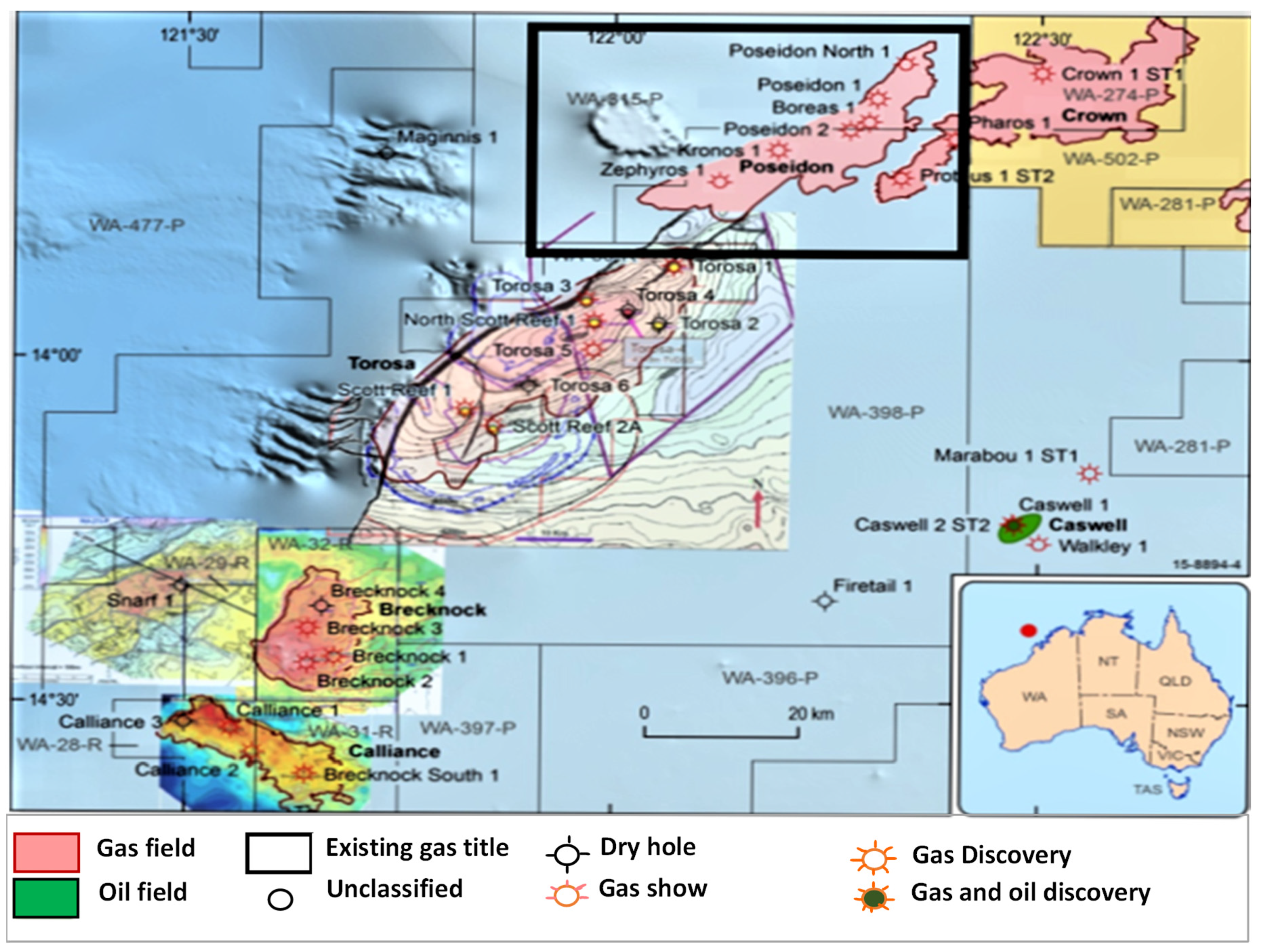
The Australian North-West Shelf (NWS) Browse Basin is a passive continental margin that stretches between the latitudes of 21° and 13° S from the SW to the NE. The Browse Basin is located in the southern edge of the Timor Sea, between the Scott Plateau to the west, the offshore Kimberley Block to the north, and the Scott Plateau to the east. It covers an area of over 140,000 km
2, and its sedimentary depth exceeds 15 km (
Figure 1). On the NWS, it is one of several lengthy sedimentary basins. The area evolved via six geological periods, from early Carboniferous to Late Jurassic inversion to late Cretaceous inversion. Thermal subsidence occurred during the Permian and Triassic ages. The center Browse Basin is a margin-parallel half-graben system that dips towards the continent structurally [
37]. The break-up of Greater India from Western Australia resulted in either a single phase or two phases of rifting, which led to the development of the NWS [
38]. A thick succession of passive edge sediment was deposited in the Browse Basin after tectonic activity in the Aptian had halted, burying the old structural relief [
39]. Several petroleum systems have been determined, implying that at least three major petroleum systems exist.
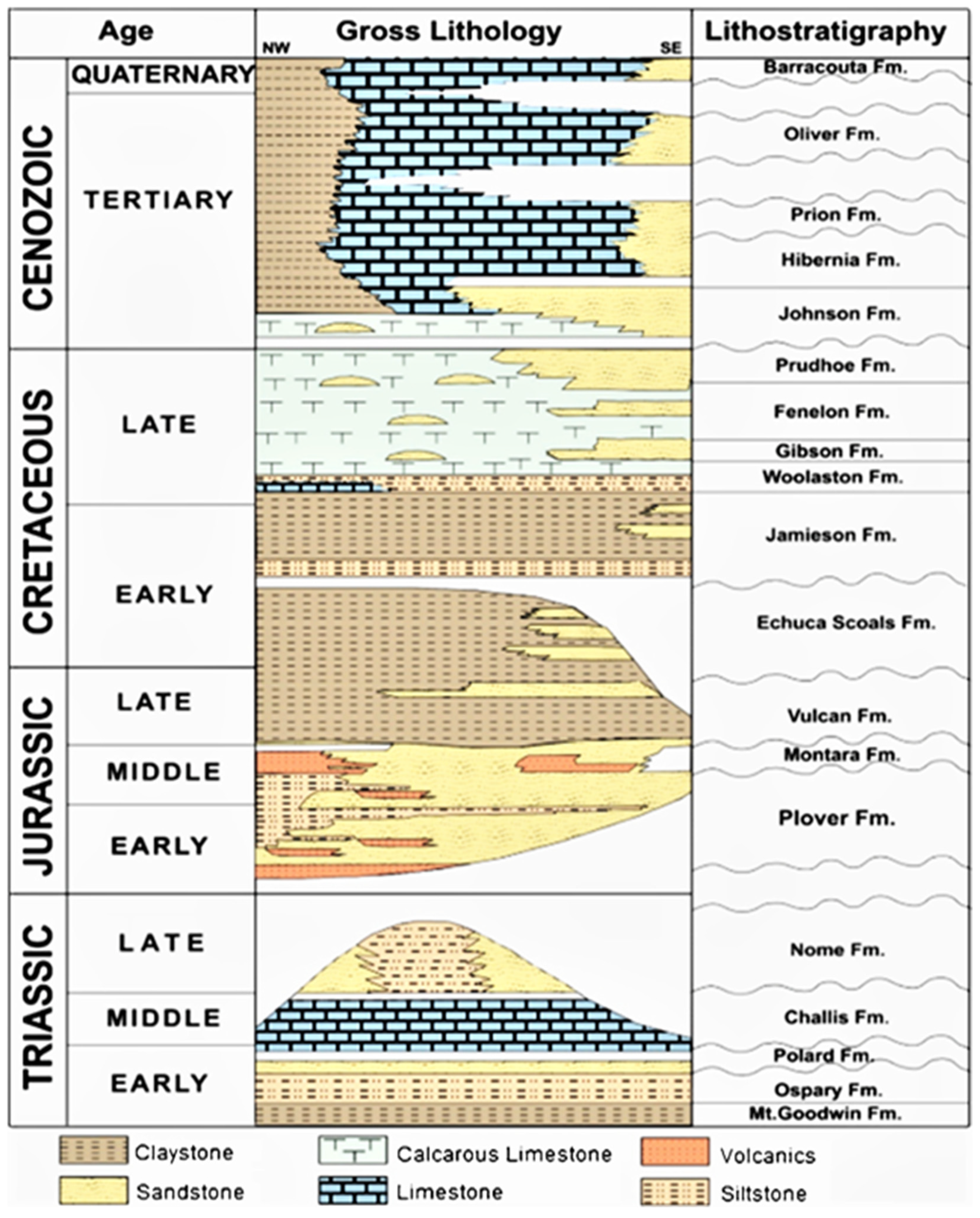
The primary structural patterns in the Browse Basin were likely produced by the final stage of rifting that occurred in the Middle Jurassic-Early Cretaceous (
Figure 2). A large and tidally dominated the Plover Formation is made up of a series of stacked fluvio-deltaic and shallow marine sands, shales, and silts, as well as trace amounts of carbonate and volcanic materials during active faulting of the Jurassic extension [
40]. As a result, the thickness and lateral continuity of this formation, ranges approximately 200 - 450 m thick sandstone are extensively variable throughout the basin. A regional unconformity is marked at the base of Plover formation whereas the top of plover is defined as Late Callovian age Unconformity. A significant volcanic province is present in the Browse Basin throughout the Early to Late Jurassic [
41]. The majority of traps forms in the area are structural, however there is potential for chronological traps on the margins of existing structures and an also alluvial/submarine fans dumped on the hanging wall of significant horsts. The rifting was connected with volcanic activity, which might deteriorate reservoir quality and absorb habitation space, inhibiting sandstone deposition [
40]. The research area’s source rocks were deposited in the broad fluvial-deltaic channels that spanned most of the basin. Prodelta shales, coaly shales, and shallow coals harbouring abundant marine organic materials are examples. Applying well data, the Near Top Plover Formation has been examined and is interpreted as an upward trend increasing in acoustic impedance. The structure of the rocks above and below this barrier is thought to be varied, with the possibility of sand on shale, shale on shale, and shale on sand interfaces. As a result, the seismic marker at the Near Top Plover Formation varies [
40]. The Near Top Plover horizon is distinguished by a rise underlying complex faulting. Normal faulting is produced in a sequence of fault ridges and grabens. This makes detecting and delineating the Plover formation’s gas saturated reservoir extremely challenging for this Browse Basin [
42].
3. Materials and Methods
3.1. Dataset
The available data for this study were provided by “The Society of Exploration of Geophysicists”. The data set includes 3D seismic data in SEG-Y format that have 1600 and 1800 number of inlines and crosslines with sample interval 4ms and number of samples per trace 501. The in-lines interval is 18.75 m whereas the crossline interval is 12.50 m. Also, the time interval of this seismic cropped volume is from 2000ms to 4000ms with normal polarity.
The dataset also includes six wells (Boreas-1, Kronos-1, Pharos-1, Poseidon-1, Poseidon-2, Proteus-1) with petrophysical logs in ASCII format, formation markers, deviation survey and five velocity check-shots in ASCII format were used to conduct a rigorous study on the structural model of Poseidon field of Browse basin. Five types of wireline logs (gamma ray, resistivity, density, neutron and sonic logs) are available with this data set.
3.2. Methodology
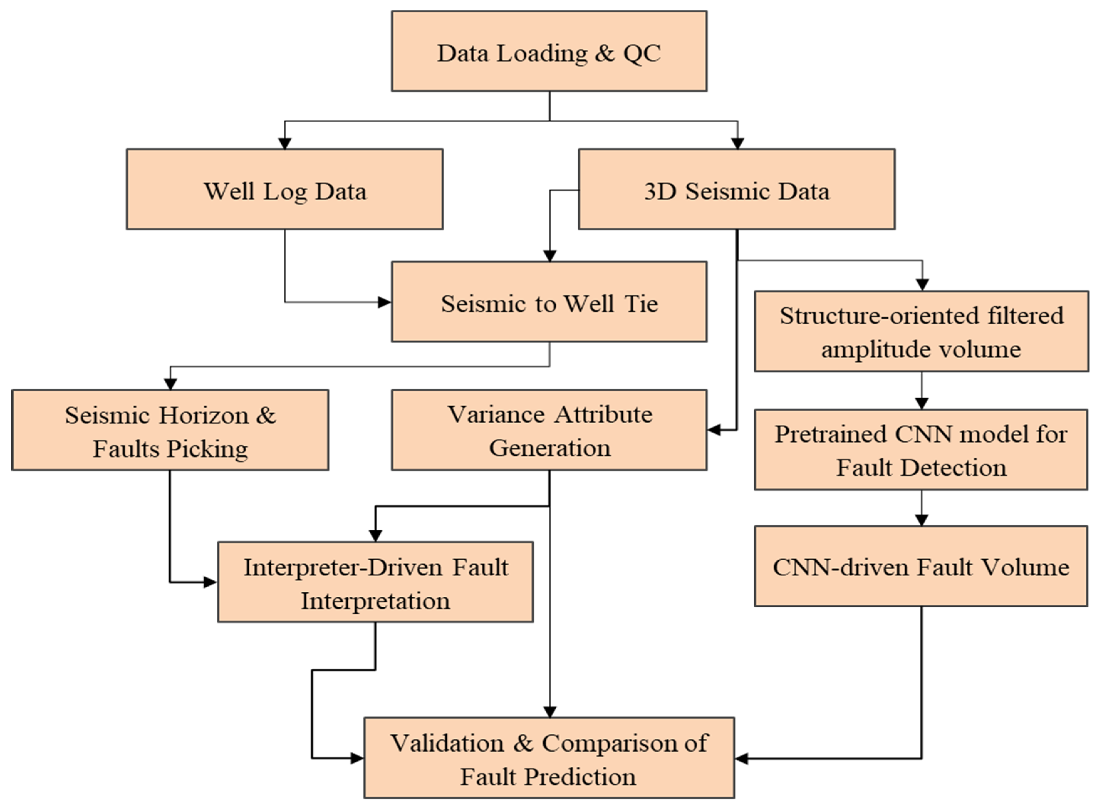
The steps taken to complete the study is shown in the workflow in
Figure 3. The 3D seismic cube and interpretation of seismic horizons and faults were used to check fault connectivity. This study started by well correlation, then establishing a good seismic to well tie followed by horizon picking and faults interpretation to generate time structure maps and fault polygons. The gamma ray and resistivity logs where mainly used for well-to-well correlation, lithology discrimination, depositional facies interpretation whereas the combination of neutron- density logs were used for fluid discrimination. Two horizons at the Plover reservoir were interpreted.
3.2.1. Interpreter Driven Horizons and Faults Interpretation
The first step was tying well data (depth domain) to seismic data (time domain) incorporating deviation and check shot surveys. Density logs, along with the sonic logs, were used to calculate the acoustic impedance (AI). An optimum wavelet was extracted and used in the synthetic generation. The cropped 3D Poseidon seismic cube has 1800 crosslines and 1600 in-lines. Both the Top and Base of Plover formation were picked. Because of structural complexity of the area, manual picking was employed. The fault blocks movements affect hydrocarbon traps and pathways in addition to deforming sedimentary basins. For the movement of hydrocarbons, faults serve as either structural traps or conduits [
44]. That is why a structural framework fault interpretation is crucial. The faults were mapped manually in software using the “interpreted fault” tool.
3.2.2. Variance attributes Generation
Variance attribute which is an edge detection technique that measures the similarity of waveforms over the lateral or vertical windows. It plays an important role for mapping channels and faults identification and is also applied to view the major fault zone, unconformities fractures and the major sequence boundaries directly. In this study, before applying this attribute, structural smoothing has been applied using 3D gaussian filter to reduce noise of the input data.
3.2.3. Deep Learning Based Fault prediction
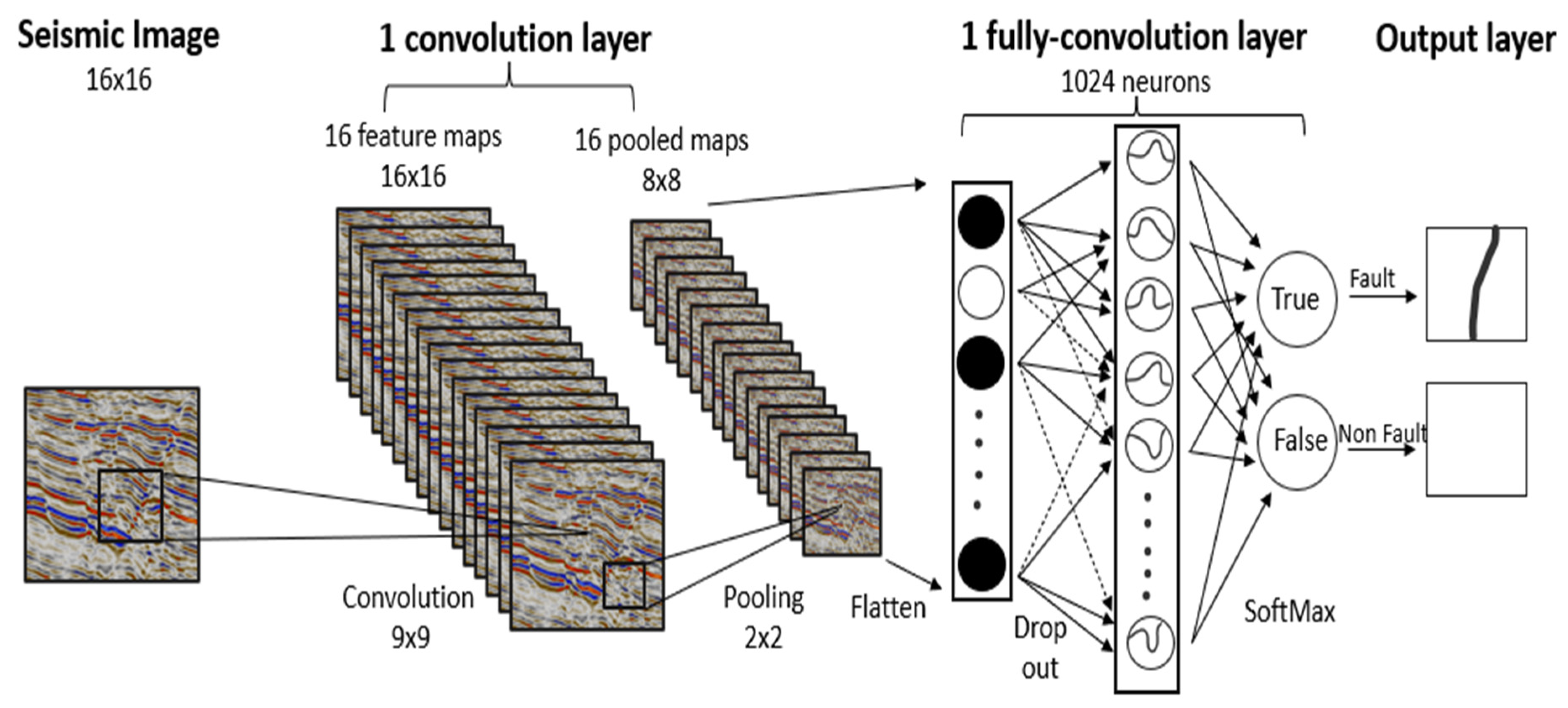
A pretrained convolutional neural network (CNN) model have been used for seismic fault identification. The CNN network identifies, learns, and categorizes the faults through locally reflected seismic patterns, allowing for the effective identification and exclusion from processing artifacts and seismic noises. For the next step, the CNN platform completes the mapping relation using original seismic amplitude between faults and seismic signals. So that, it can be applicable to the large data sets without any repetition in selection of attributes and guide as a shield to the interpreters from complexity. The output from this network is extracting a single value that is represented by a binary label defined as “Fault” or “Non-Fault”.
In this study, the pretrained convolution neural network (CNN) model is run on the full 3D seismic volume of Poseidon field after several iteration of pre-conditioning namely structurally oriented filtering (SOF3D) to sharpen and improve the discontinuities in the amplitude volume. This pre-conditioning helps to remove noisy from the dataset. The volume of conditioned amplitude data is then sent into the CNN algorithm. Three different U-net architecture model operated on the data known as aggressive, conservation and mixed angle engine. Only the result of mixed angle engine was found to be geologically acceptable.
4. Results and Discussion
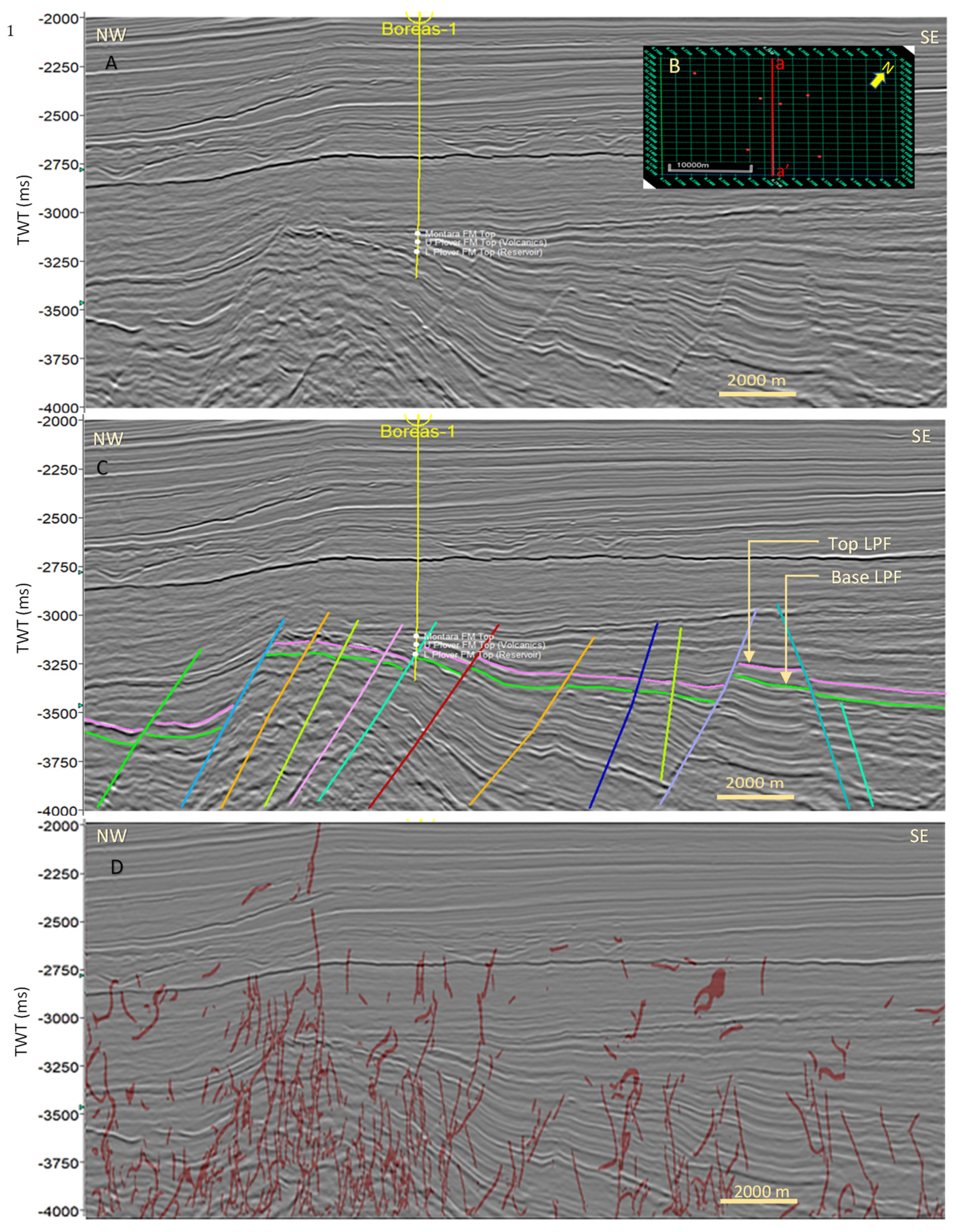
3D seismic does not usually offer sharp imaging of faults and is sometimes ambiguous regarding fault geometry and continuity. The two interpreted horizons are shown in
Figure 4. In this study a variance cube was created to confirm and enhance the manually picked faults on original seismic inline-2940 shown in
Figure 5(C).
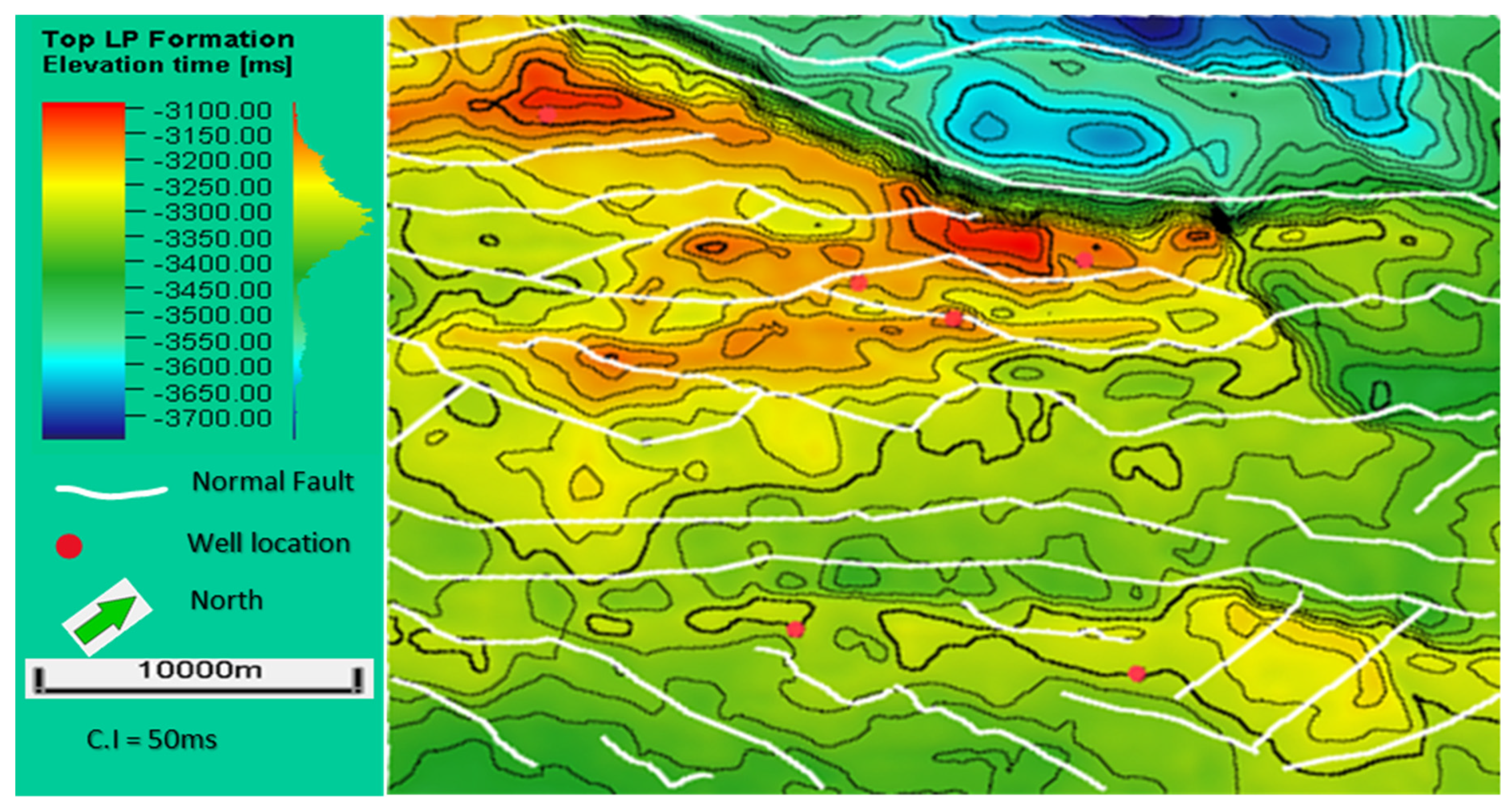
Fault polygons were created manually after picking horizon of top and base of Lower Plover formation (LPF) and TWT structure map was generated from the picked horizons (
Figure 6). From the structure map it is observed that majority of the faults are trending NW to SE direction. The reservoir zone lies between 3250ms to 3500ms on average, but the northern block is down faulted to about 3700ms.
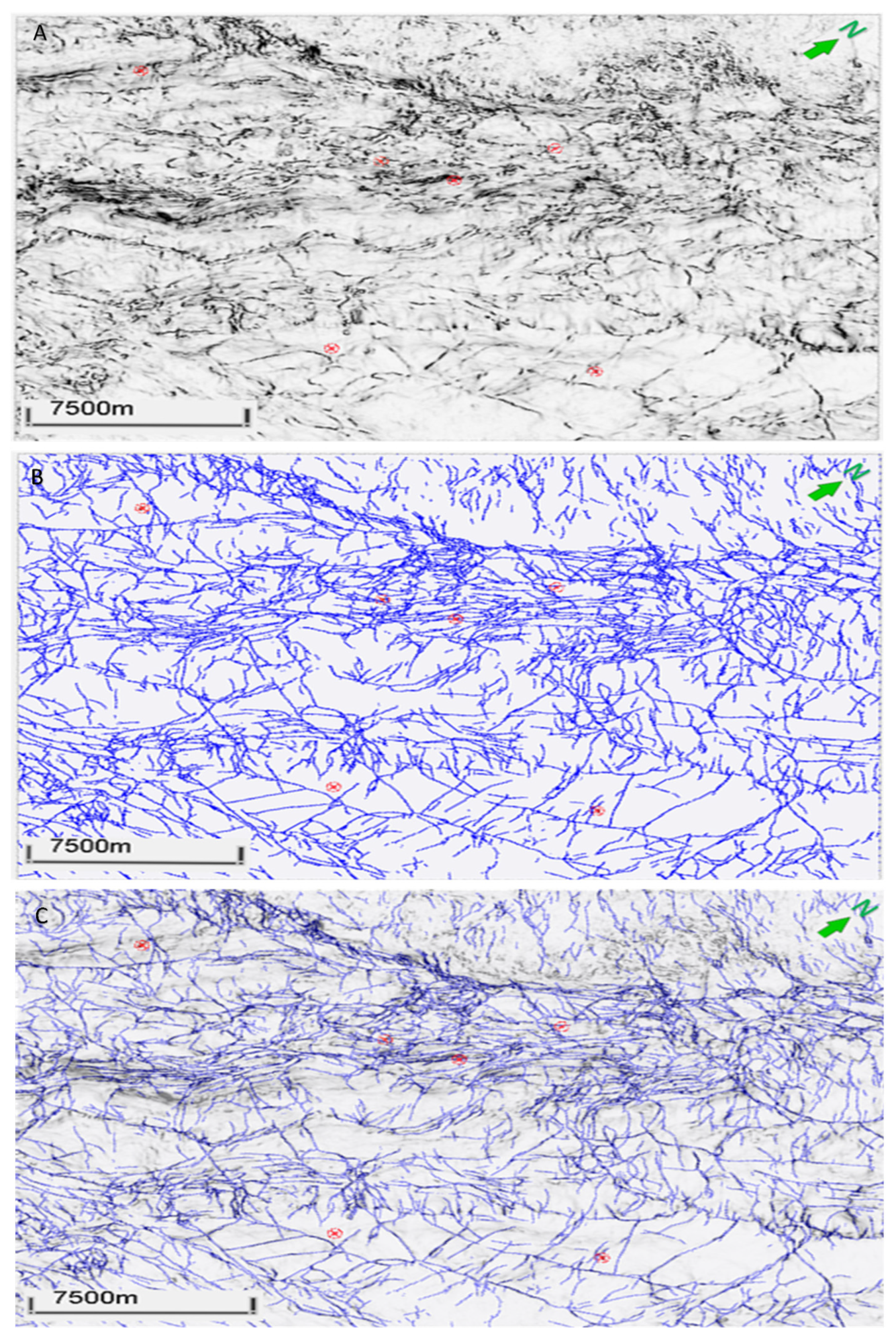
Deep learning (DL) auto-fault detection convolution neural network (CNN) algorithm was also applied to same 3D. The DL identified faults will be compared to the conventionally picked faults and variance lineaments. It is important to mention that most of the faults identified by variance and/or DL can be interpreted using the conventional and manual picking but obviously is more time consuming demanding high interpretation skills in addition to structural geology domain experience. Deep Learning fault identification are shown in
Figure 7(B) on inline 2940
There were three fault interpretation cases observed and investigated on both Variance and DL auto fault detection.
Case-1 represents faults that are clearly visible on both Variance and DL, Case-2 represents faults that are clearly visible in DL but not in Variance and lastly and Case-3 where faults are visible in Variance but not detected or identified on DL. In the following sections, a few examples from each case are shown.
To facilitate the comparisons, a time slice at 3464ms from both variance and DL cubes (
Figure 7) was selected due to its proximity to horizon top Plover Formation. A few 3D arbitrary seismic sections crossing some faults were selected to demonstrate the clarity of events termination for fault detection.
Case 1: Faults clearly visible on both Variance and DL cubes
As expected, almost all the faults fell in this category. A few examples were selected to be presented. In
Figure 8, clear continuous N-S trending fault (
F) seen on DL (E) whereas it is seen as two disconnected segments on variance. In the vertical sections the faults show clearly. Spatial fault continuity is not clear on the variance slice as compared to that of the DL. Another 3D arbitrary seismic section that crosses the gap between the two variance fault segments clearly shows the event terminations.
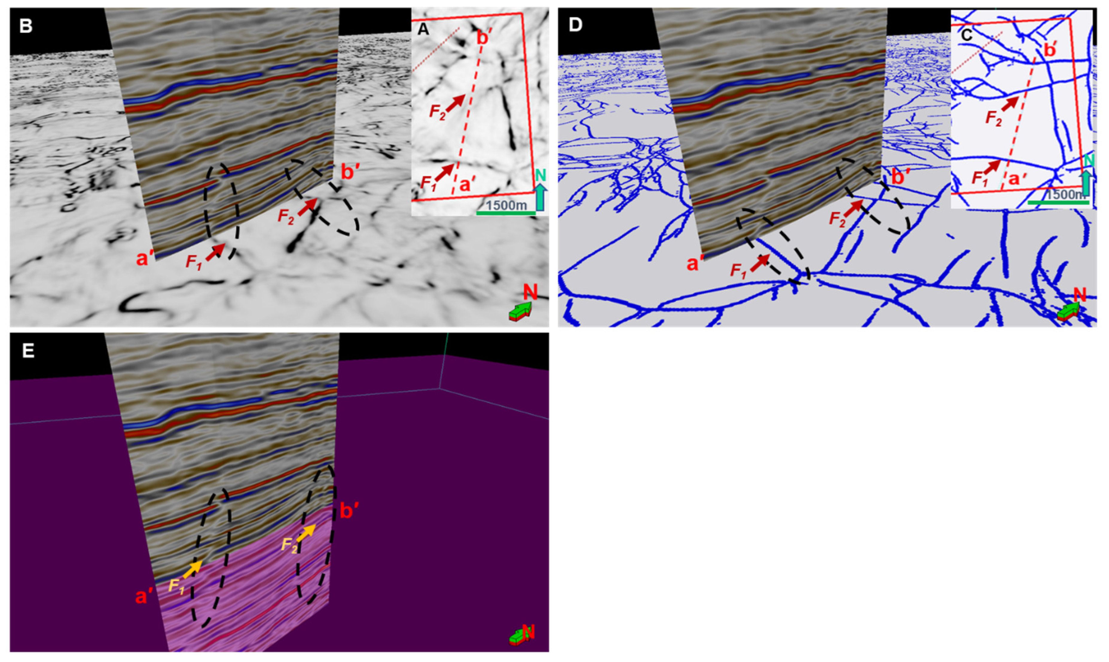
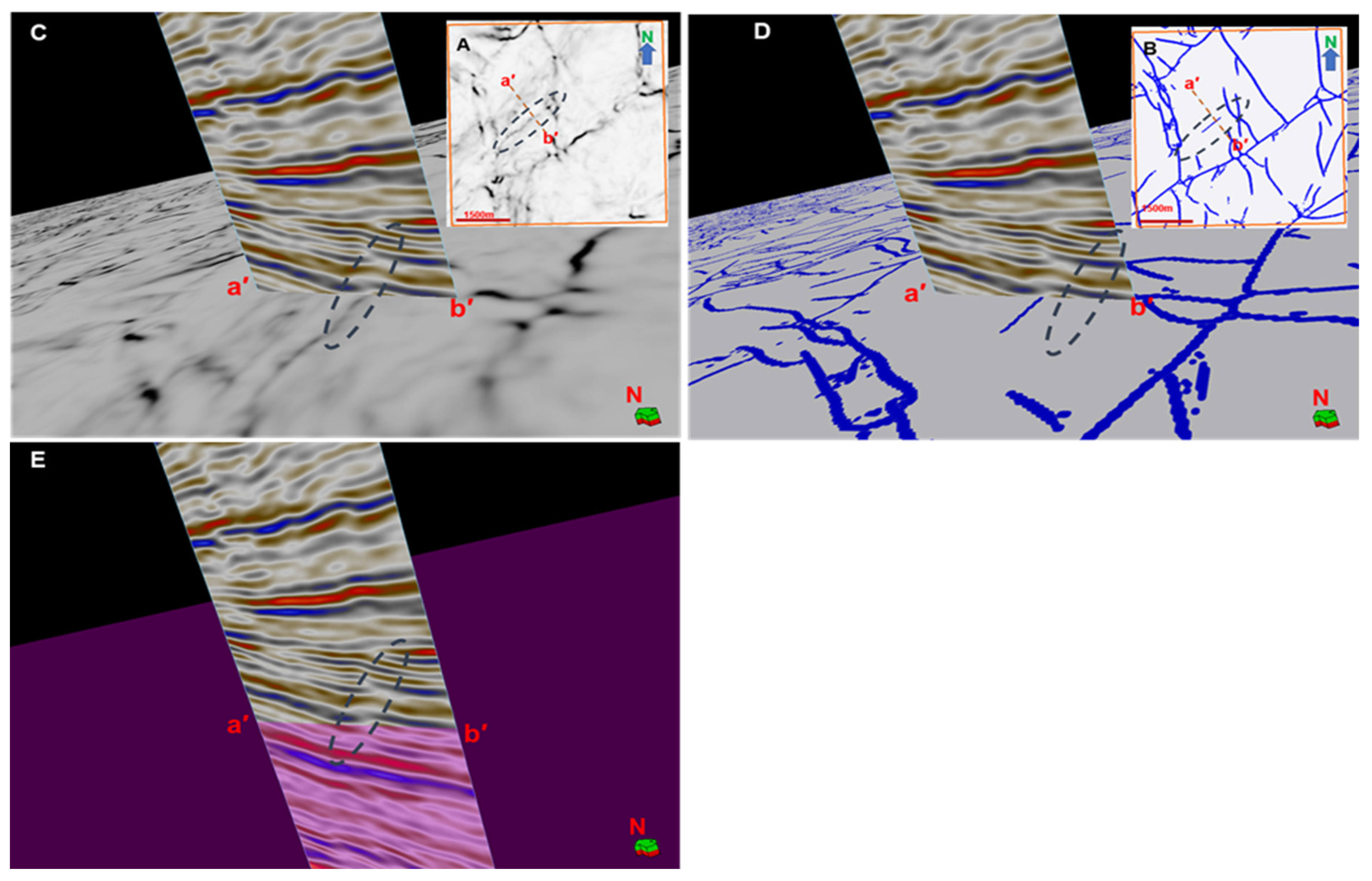
In
Figure 9, a different area showing two faults detected on both Variance and DL fault-auto detection. On the vertical seismic section (a′-b′) F
1 fault is clearly seen whereas F
2 fault is not. It is observed that a fault detected on the DL time slice (F
2) is not observed on the vertical seismic section. On the other hand, that same fault (F
2) also not observed on the variance slice. This raises a question as to the validity of the detected lineament on the DL slice.
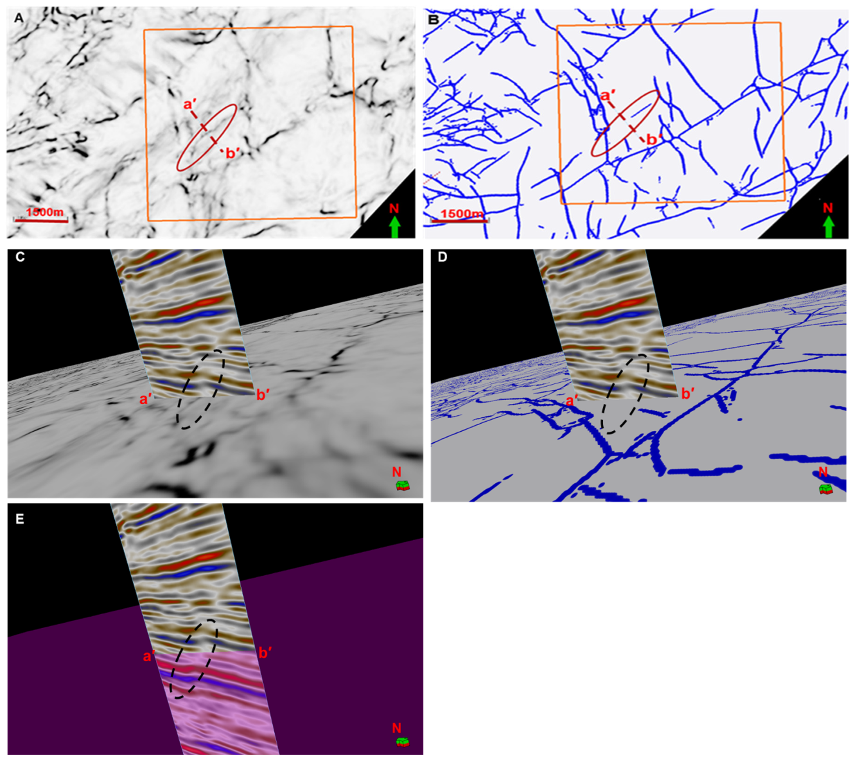
In
Figure 10 is a fault detected on both variance and DL. The lateral extent of the fault on the DL slice is quite shorter than that seen on the variance slice, even though the fault is quite distinct on the vertical seismic section.
Case 2: Faults clearly visible DL and not in Variance cubes
This case demonstrates the value of DL identified lineaments that are not detected by the variance.
Figure 11 represents an example of fault is detected on both variance and DL, but does not extend far enough on the variance, even though it is quite clear on the vertical seismic section (a′-b′).
Case 3: Faults clearly visible on variance but not on DL cubes
In
Figure 12, the fault under consideration is seen in variance cube but does not exist in the DL slice. The vertical section supports the existence of the fault, which was missed on the DL slice.
6. Conclusions
Accurate identification of faults and fractures from 3D seismic data is an essential stage for subsurface interpretation and reservoir characterization. In this study, we used convolutional neural network (CNN) model that was pre-trained with synthetic data to predict seismic faults using 3D seismic volume. The fault probability result using the real dataset performed better compared to manual interpretation with the variance attribute. Based on the results, there were three seismic interpretation scenarios observed in the deep learning automated fault prediction and variance attribute. Although most of the major faults identified on DL are seen on the variance cube, some minor faults are seen on one and not on the other. The automated fault identification using the pre-trained CNN on seismic dataset significantly cut down on the time and resources needed to interpret faults by getting quick results on the full seismic volume.
Author Contributions
Conceptualization, M.M.I., I.B, and M.E; methodology, M.M.I., I.B, and M.E; software, M.M.I., I.B, and M.E; validation, M.M.I., I.B, M.E and S.E.; formal analysis, M.M.I., M.E, S.E., N.A.S. and I.B.; investigation, M.E.; resources, M.E.; data curation, M.E.; writing—original draft preparation, M.M.I.; writing—review and editing, , M.M.I., M.E, S.E., N.A.S. and I.B.; visualization, M.E.; supervision, M.E.; project administration, M.E.; funding acquisition, M.E. All authors have read and agreed to the published version of the manuscript.
Funding
This research was supported through the following project: “Machine Learning Application in lithology and fluid properties Prediction utilizing seismic and well log data for optimal reservoir characterization” with cost center: 015LC0-420, grant type: YUTP-FRG 1/2022.
Institutional Review Board Statement
Not Applicable.
Informed Consent Statement
Not Applicable
Data Availability Statement
Acknowledgments
The authors would like to thank PETRONAS for funding this project. We thank SLB for giving Petrel software that we used for seismic interpretation and visualization. Our thanks also go to Geophysical Insights for donating Paradise software that we used for deep learning-based fault prediction. Many thanks go to the editors and reviewers for providing insightful suggestions on improving the paper quality.
Conflicts of Interest
The authors acknowledge no conflict of interest. The funders had no role in the structure of the study; in acquiring, analyzing, or interpreting of data; in the composition of the manuscript, or in the decision to publish the results.
References
- H. M. Basir, A. Javaherian, and M. T. Yaraki, “Multi-attribute ant-tracking and neural network for fault detection: A case study of an Iranian oilfield,” Journal of Geophysics and Engineering, vol. 10, no. 1, 2013. [CrossRef]
- A. Cunha, A. Pochet, H. Lopes, and M. Gattass, “Seismic fault detection in real data using transfer learning from a convolutional neural network pre-trained with synthetic seismic data,” Computers & Geosciences, vol. 135, p. 104344, 2020/02/01/ 2020. [CrossRef]
- H. Di, Z. Wang, and G. AlRegib, “Seismic Fault Detection from Post-Stack Amplitude by Convolutional Neural Networks,” vol. 2018, no. 1, pp. 1-5, 2018. [CrossRef]
- D. A. Otchere et al., “Improving seismic fault mapping through data conditioning using a pre-trained deep convolutional neural network: A case study on Groningen field,” Journal of Petroleum Science and Engineering, vol. 213, 2022. [CrossRef]
- C. E. Bond, “Uncertainty in structural interpretation: Lessons to be learnt,” Journal of Structural Geology, vol. 74, pp. 185-200, 2015. [CrossRef]
- J. Alcalde, C. E. Bond, G. Johnson, J. F. Ellis, and R. W. Butler, “Impact of seismic image quality on fault interpretation uncertainty,” GSA Today, 2017. [CrossRef]
- S. Oumarou et al., “Seismic attributes in reservoir characterization: An overview,” Arabian Journal of Geosciences, vol. 14, pp. 1-15, 2021. [CrossRef]
- S. Chopra and K. J. Marfurt, Seismic Attributes for Prospect Identification and Reservoir Characterization. Society of Exploration Geophysicists, 2007. [CrossRef]
- F. Neves, M. Zahrani, and S. Bremkamp, “Detection of potential fractures and small faults using seismic attributes,” The Leading Edge, vol. 23, pp. 903-906, 09/01 2004. [CrossRef]
- X.-L. Wei et al., “Seismic fault detection using convolutional neural networks with focal loss,” Computers & Geosciences, vol. 158, p. 104968, 11/01 2021. [CrossRef]
- Z. Yan, Z. Zhang, and S. Liu, “Improving Performance of Seismic Fault Detection by Fine-Tuning the Convolutional Neural Network Pre-Trained with Synthetic Samples,” Energies, vol. 14, p. 3650, 06/19 2021. [CrossRef]
- T. Boe and R. Daber, Seismic features and the human eye: RGB blending of azimuthal curvatures for enhancement of fault and fracture interpretation. 2010, pp. 1535-1539. [CrossRef]
- X. Wu and D. Hale, 3D seismic image processing for faults (conference paper). 2015. [CrossRef]
- P. P. Van Bemmel and R. E. Pepper, “Seismic signal processing method and apparatus for generating a cube of variance values,” ed: Google Patents, 2000.
- K. J. Marfurt, R. L. Kirlin, S. L. Farmer, and M. S. Bahorich, “3-D seismic attributes using a semblance-based coherency algorithm,” Geophysics, vol. 63, no. 4, pp. 1150-1165, 1998. [CrossRef]
- K. J. Marfurt, V. Sudhaker, A. Gersztenkorn, K. D. Crawford, and S. E. Nissen, “Coherency calculations in the presence of structural dip,” Geophysics, vol. 64, no. 1, pp. 104-111, 1999. [CrossRef]
- A. Gersztenkorn and K. J. Marfurt, “Eigenstructure-based coherence computations as an aid to 3-D structural and stratigraphic mapping,” Geophysics, vol. 64, no. 5, pp. 1468-1479, 1999. [CrossRef]
- S. Wang, S. Yuan, B. Yan, Y. He, and W. Sun, “Directional complex-valued coherence attributes for discontinuous edge detection,” Journal of Applied Geophysics, vol. 129, pp. 1-7, 2016. [CrossRef]
- R. L. Kirlin, “The relationship between semblance and eigenstructure velocity estimators,” Geophysics, vol. 57, no. 8, pp. 1027-1033, 1992. [CrossRef]
- D. Hale, “Methods to compute fault images, extract fault surfaces, and estimate fault throws from 3D seismic images,” Geophysics, vol. 78, no. 2, pp. O33-O43, 2013. [CrossRef]
- Q. S. Imran et al., “Automated fault detection and extraction under gas chimneys using hybrid discontinuity attributes,” Applied Sciences, vol. 11, no. 16, p. 7218, 2021. [CrossRef]
- M. Kim, J. Yu, N.-K. Kang, and B.-Y. Kim, “Improved Workflow for Fault Detection and Extraction Using Seismic Attributes and Orientation Clustering,” Applied Sciences, vol. 11, no. 18, p. 8734, 2021. [CrossRef]
- Cohen, N. Coult, and A. A. Vassiliou, “Detection and extraction of fault surfaces in 3D seismic data,” Geophysics, vol. 71, no. 4, pp. P21-P27, 2006. [CrossRef]
- H. Di and D. Gao, “3D seismic flexure analysis for subsurface fault detection and fracture characterization,” Pure and Applied Geophysics, vol. 174, pp. 747-761, 2017. [CrossRef]
- X. Qi and K. Marfurt, “Volumetric aberrancy to map subtle faults and flexures: 87th Annual International Meeting, SEG, Expanded Abstracts, 3443–3447,” ed, 2017. [CrossRef]
- A. A. Aqrawi and T. H. Boe, “Improved fault segmentation using a dip guided and modified 3D Sobel filter,” in SEG Technical Program Expanded Abstracts 2011: Society of Exploration Geophysicists, 2011, pp. 999-1003. [CrossRef]
- A. Iske and T. Randen, Mathematical methods and modelling in hydrocarbon exploration and production. Springer, 2006. [CrossRef]
- I. Cohen and R. R. Coifman, “Local discontinuity measures for 3-D seismic data,” Geophysics, vol. 67, no. 6, pp. 1933-1945, 2002. [CrossRef]
- H. Di and D. Gao, “Gray-level transformation and Canny edge detection for 3D seismic discontinuity enhancement,” Computers & Geosciences, vol. 72, pp. 192-200, 2014. [CrossRef]
- E. Rijks and J. Jauffred, “Attribute extraction: An important application in any detailed 3-D interpretation study,” The Leading Edge, vol. 10, no. 9, pp. 11-19, 1991. [CrossRef]
- S. Al-Dossary and K. J. Marfurt, “3D volumetric multispectral estimates of reflector curvature and rotation,” Geophysics, vol. 71, no. 5, pp. P41-P51, 2006. [CrossRef]
- B. Zhang, Y. Liu, M. Pelissier, and N. Hemstra, “Semiautomated fault interpretation based on seismic attributes,” Interpretation, vol. 2, no. 1, pp. SA11-SA19, 2014. [CrossRef]
- G. Machado, A. Alali, B. Hutchinson, O. Olorunsola, and K. J. Marfurt, “Display and enhancement of volumetric fault images,” Interpretation, vol. 4, no. 1, pp. SB51-SB61, 2016. [CrossRef]
- H. Di, M. A. Shafiq, and G. AlRegib, “Seismic-fault detection based on multiattribute support vector machine analysis,” in 2017 SEG International Exposition and Annual Meeting, 2017: OnePetro. [CrossRef]
- H. Di, M. Shafiq, and G. AlRegib, “Patch-level MLP classification for improved fault detection,” in SEG Technical Program Expanded Abstracts 2018: Society of Exploration Geophysicists, 2018, pp. 2211-2215. [CrossRef]
- T. Zhao, V. Jayaram, A. Roy, and K. J. Marfurt, “A comparison of classification techniques for seismic facies recognition,” Interpretation, vol. 3, no. 4, pp. SAE29-SAE58, 2015. [CrossRef]
- H. I. Struckmeyer, J. E. Blevin, J. Sayers, J. M. Totterdell, K. Baxter, and D. L. Cathro, “Structural evolution of the Browse Basin, North West Shelf: New concepts from deep-seismic data,” 1998.
- A. Kaiko and A. Tait, “Post-rift tectonic subsidence and palaeo-water depths in the Northern Carnarvon Basin, Western Australia,” The APPEA Journal, vol. 41, no. 1, pp. 367-379, 2001.
- M. Apthorpe, “Cainozoic depositional history of the North West Shelf,” in The North West shelf, Australia. Symposium, 1988, pp. 55-84. [CrossRef]
- M. Farfour, M. A. K. El-Ghali, S. Gaci, M. S. H. Moustafa, and N. A. Siddiqui, “Seismic attributes for hydrocarbon detection and reservoir characterization: A case study from Poseidon field, Northwestern Australia,” Arabian Journal of Geosciences, vol. 14, no. 24, p. 2814, 2021/12/09 2021. [CrossRef]
- N. Hoffman, K. Hill, G. Ellis, P. Baillie, and T. Munson, “Structural-stratigraphic evolution and hydrocarbon prospectivity of the deep-water Browse Basin, North West Shelf, Australia,” in Timor Sea Petroleum Geoscience. Proceedings of the Timor Sea Symposium, Darwin, 2003, pp. 19-20.
- M. Farfour and D. Foster, “Machine learning and seismic attributes for prospect identification and risking: An example from offshore Australia,” in SEG/AAPG International Meeting for Applied Geoscience & Energy, 2022: OnePetro. [CrossRef]
- S. R. Le Poidevin, P. Temple, D. Saint Edwards, and T. Kuske, Australian Petroleum Accumulations Report 7 Browse Basin: Western Australia and Territory of Ashmore and Cartier Islands Adjacent Area. Geoscience Australia, 2015. [CrossRef]
- A. Gartrell, Y. Zhang, M. Lisk, and D. Dewhurst, “Fault intersections as critical hydrocarbon leakage zones: Integrated field study and numerical modelling of an example from the Timor Sea, Australia,” Marine and Petroleum Geology, vol. 21, pp. 1165-1179, 11/01 2004. [CrossRef]
- H. Di, A. Shafiq, Z. Wang, and G. Alregib, “Improving seismic fault detection by super-attribute-based classification,” Interpretation, vol. 7, pp. 1-56, 06/03 2019. [CrossRef]
|
Disclaimer/Publisher’s Note: The statements, opinions and data contained in all publications are solely those of the individual author(s) and contributor(s) and not of MDPI and/or the editor(s). MDPI and/or the editor(s) disclaim responsibility for any injury to people or property resulting from any ideas, methods, instructions or products referred to in the content. |
© 2023 by the authors. Licensee MDPI, Basel, Switzerland. This article is an open access article distributed under the terms and conditions of the Creative Commons Attribution (CC BY) license (http://creativecommons.org/licenses/by/4.0/).
