Improved Sea Ice Image Segmentation using U²-Net and Data Set Augmentation

1. Introduction

Sea ice has a substantial impact on global climate change, geophysical activities such as ocean surface physical properties and currents, and economic and social activities such as maritime shipping and transportation [1]. The freezing and thawing of sea ice and sea ice drift in winter interfere with sea-related engineering, marine trade, and various offshore industrial production activities to varying degrees. Internationally, the melting of Arctic sea ice is intensifying due to global warming, and the Arctic shipping route connecting the Atlantic Ocean and the Pacific Ocean will soon open, shortening the voyage from the eastern coast of China to the east coast of the United States (instead of the Panama Canal) by at least two thousand nautical miles, and reducing the distance from the northern port of China to the western and northern coastal ports of Europe by 25–55% [2]. Therefore, sea ice monitoring is important for maritime shipping, environmental changes, and disaster prevention.

Currently, sea ice segmentation methods can be roughly divided into three types: threshold segmentation, machine learning, and deep learning. For example, Wang used multiple thresholding and random forest methods to invert FY-4A Bohai Sea regional images and introduced a seed-filling algorithm to revise the results, which improved the accuracy of sea ice inversion under non-clear sky conditions [4]. Li proposed turbid seawater end elements for Bohai Sea ice and water classification, used multi-feature binomial tree classification to solve the problem of the difficult distinction between turbid seawater and sea ice and used mixed-image element decomposition to enter the pixel interior to analyze its category [5]. Li et al. proposed an AL-TSVM sea ice image classification method from the perspective of combining active learning with semi-supervised learning by combining a small amount of labeled, known training data and the overall data feature and spatial distribution patterns [6]. Han et al. obtained a combination of informative and low-similarity superior bands using the mutual information similarity metric and classified them using a support vector machine [7]. Zhou et al. improved the OSSP algorithm in three aspects: training set composition, classification result output, and tilted image geometry correction, to improve the classification accuracy of ship-based images [8]. Yu proposed a pixel-level domain relationship context classification method for sea ice spatial neighborhood relations [9].

In the field of deep learning, Dowden et al. evaluated SegNet and PSPNet101 neural networks based on self-built training and testing sets. The sea ice classification dataset consisted of 1,090 images with labels; for the test set of 104 images, the classification accuracy was 98.3% or better for both, validating the applicability of deep learning methods for sea ice detection [10]. Han et al. proposed a multilevel, feature-fusion image classification method based on a residual network PCA method to extract the first principal component of the original image, used a residual network to deepen the number of network- layer FPN, PAN, and SPP modules to increase the mining between layer and layer features, merged the features between different layers, and used the hyperspectral image of Bohai Bay for validation; the method improved the sea ice classification accuracy [11].

Shi proposed using the PCANet network to select adaptive convolutional filter banks to mine sea ice depth features, adding hash binarization mapping and chunked histograms to enhance feature separation and reduce feature dimensionality. The author designed a two-branch, multi-source, remote sensing, deep learning model for optical and SAR images to obtain good classification results with fewer training samples [12]. The improved SIS-Unet network outperformed the classical Unet network by adding a residual structure and void space pyramidal pooling structure to the Unet network 13. Cui et al. used the convolutional neural network (CNN) model for image segmentation and selected the appropriate cost and activation functions according to the principle of migration learning. They examined the HJ-1A/B Bohai Sea sea-ice images as the experimental data source labeled samples and achieved better experimental results [14]. Han et al. proposed a spectral-spatial-joint feature concept for hyperspectral sea ice image classification and designed a three-dimensional (3D-CNN) model to extract the deep spectral-spatial features of sea ice by conducting sea ice classification experiments using two hyperspectral datasets, Baffin Bay and Bohai Bay, with experimental results based on a single-feature CNN algorithm [15]. Han et al. used the advantage of a CNN in deep feature extraction to design a deep learning network structure for SAR and optical images to achieve sea ice image classification by feature extraction and feature-level fusion of heterogeneous data; the effectiveness of the method was verified using two sets of heterogeneous satellite data in the Hudson Bay area [16]. Zhang et al. classified the Beaufort Sea and Severnaya Zemlya based on a Micro Sea Ice Residual Convolution Network (MSI-ResNet); the MSI-ResNet method performed better than the traditional support vector machine (SVM) classifier for identifying sea ice [17]. Cheng Wen et al. proposed an automatic LFSI extraction method for the Laptev Sea in the eastern Arctic Ocean based on the conditional generative adversarial network Pix2Pix and validated it experimentally using true color images from the Moderate Resolution Imaging Spectroradiometer (MODIS) [18].

In terms of data augmentation, Liu et al. proposed a data augmentation method based on image gradients, which can freely choose the number of expansions and image sizes to effectively expand the dataset, and demonstrated through comparison experiments that the accuracy of the network model was improved after expanding the dataset by this method; the improvement was more obvious when the dataset was small, and the model accuracy could be improved by effectively reducing overfitting. The improvement is more obvious in the case of small datasets and can effectively reduce overfitting to improve the model accuracy. Ziqi et al. fused random probability resampling with adaptive scale equalization, added the fusion expansion algorithm to different target detection algorithms for experiments, and verified that the expansion algorithm can effectively reduce misdetection and false detection of small targets in road scenes. By improving the generator and the discriminator of the Wasserstein–Generative Adversarial Network (W-GAN) and introducing reconstruction and perceptual style loss to enhance the ability of generating remote sensing images by ship, Yang et al. used the remote sensing images generated by ship-WGAN to train the image recognition model, and the recognition accuracy was substantially improved by sample expansion of the generated samples to achieve the effect of data augmentation. The recognition accuracy was substantially improved by expanding the generated samples, and data enhancement was achieved.

Sea ice dataset labeling requires manual interpretation and mapping, and relies on ship-based and shore-based observations, which are costly. In this context, to obtain the segmentation of sea ice remote sensing images under limited sample conditions and achieve good generalization of the semantic segmentation model, this study improved two aspects of data augmentation and network structure, and used a test set to check the accuracy of the improved model.

2. Materials and Methods

2.1. Data Augmentation

Difficulty in acquiring optical images of sea ice, the high cost of labeling, and an insufficient number of samples are obstacles to sea ice segmentation, classification, and detection. Owing to complex sensor factors and special weather conditions, image noise and cloud occlusion are major obstacles to the inversion of optical sea ice images. Image augmentation is an effective method for solving data limitations in deep-learning model training. Data augmentation not only increases the number of samples in the dataset but also improves the generalization ability of neural networks. The main data augmentation methods used in this study were affine transform, fuzzy, mirror image, noise, and optical spatial transform augmentations.

In noisy data augmentation experiments, the Gaussian random noise is representative of noise type in image processing. In this study, we used the Box–Muller transform method to generate Gaussian random noise and studied the effects of noise with different parameters on the model accuracy and generalization ability. The principle is: the joint two-dimensional distribution of two mutually independent Gaussian random numbers with zero mean and the same variance is radially symmetrical, and the Gaussian random number output by the algorithm can be considered to be the coordinates of a random point in the two-dimensional plane, the amplitude of which is transformed from a random number obeying a uniform distribution on the interval. Its phase is obtained by multiplying a uniform random number on the interval, and the random point is mapped onto the Cartesian coordinate axis. The corresponding coordinate point is a random number that follows a Gaussian distribution.

X and Y are assumed to obey normal distributions and the random variables, X and Y, are transformed as (Equations (1) and (2)):

$$X=R\cos (\theta )$$

(1)

$$Y=R\sin (\theta )$$

(2)

The distribution functions are described by Equations (3)–(5):

$$P_R(R\le r)={\displaystyle {\int }_0^{2\pi }{\displaystyle {\int }_0^r\frac{1}{2\pi }}}{e}^{\frac{-R^2}{2}}Rd\theta dR=1-e^{-\frac{r^2}{2}}$$

(3)

$$P_{\theta }(\theta \le \varphi )={\displaystyle {\int }_0^{\varphi }{\displaystyle {\int }_0^{\infty }\frac{1}{2\pi }}}{e}^{\frac{-R^2}{2}}Rd\theta dR=\frac{\varphi }{2\pi }$$

(4)

$$\mathrm{Retrieved}\mathrm{from}{P}_R\mathrm{inverse}\mathrm{function}R=F_R^{-1}(1-z)=\sqrt{-2\ln (1-z})$$

(5)

When$z$ follows a uniform distribution in [0, 1], the distribution function of R is $P_R$. Thus, two random variables, U₁ and U₂, which obey a uniform distribution on [0,1], can be selected such that

$$\theta =2\pi U_1,1-z=U_2,R=\sqrt{-2\ln U_2}$$

(6)

By substituting this into equations 1 and 2, the normally distributed random quantities, X and Y, were constructed. In this study, based on this principle, Gaussian random numbers were generated from uniformly distributed, pseudo-random numbers to approximately obey a normal distribution [23].

To intuitively understand the strength of the noise, this study used the following strategy to generate the noise: first, the image grayscale value was divided by 255 to normalize to the interval [0,1]. Then a noisy image was generated with a mean value of 0 and a variance of a given value of $\sigma$. The noise and image were superimposed and set to 1 if the pixel value was greater than 1, and set to 0 if the pixel value was less than 0. Finally, the value was multiplied by 255 to map the pixel grayscale value back to 0–255. The "0.1 noise" mentioned in this paper indicates that "0.1" is the value of the parameter, $\sigma$, in the noise generation process.

The study area was the Bohai Sea ice monitoring dataset, and the dataset was the sea ice target monitoring dataset from the visible image of Ocean One. The sea ice tag images were obtained from manual mapping. The pixel depth of the images was 24 bits, the original images were in red, green, and blue channels, the tag images were 8-bit grayscale images, the sea ice area was marked as 255, and the non-sea ice area was marked as 0.

The original training set has a total of 1200 images, and the 1200 images are used as the basic unit for augmentation using image rotation, brightness variation, and noise injection, respectively, before the experiment. The training set numbers and compositions are listed in Table 1. To more accurately measure the accuracy of each model, the test set (300 frames) was expanded (90-degree rotation, 180-degree rotation, blurring, and brightening) to obtain an expanded test set (1500 frames).

2.2. U²-Net Retrofit

2.2.1. U²-Net Network and Convolutional Block Attention Module (CBAM)

The U²-Net network has the following advantages: firstly, the network is a two-layer, nested, U-shaped structure that does not use a pre-trained backbone model for image classification, and the model weights are trained from the training set; secondly, the new architecture allows the network to go deeper and obtain high-resolution features without substantially increasing memory and computational costs. In the bottom layer, a new RSU is designed to extract intra-stage, multi-scale features without reducing the feature mapping resolution. In the top layer, there is a U-Net-like structure, where each stage is populated by a ReSidual U-block. The feature map is down-sampled twice after each Encoder and up-sampled before passing through each Decoder twice before passing through each decoder. The ReSidual U-blocks in the network can be divided into two categories: Encoder1–Encoder4 and Decoder1–Decoder4. They use the same modular structure of RSU-L, only the depth (L) is different. Taking L = 7 as an example, the maximum downsampling time was 32 times. When Encoder5–6 and Decoder 6 used the module RSU-F, the main difference between the RSU-L and RSU-F structures was that there was no more downsampling (purple part). Because the image size has been sufficiently downsampled, much contextual information will be lost when the image size is decreased again, which affects image segmentation. Therefore, RSU-4F is used in the deep layer, and the module decreases the downsampling part and uses multi-layer expansion convolution to enlarge the receptive field. The right side shows the output of the fusion of the features of each layer after upsampling to obtain the segmented image as large as the original image, and the feature map of each layer is then convolved by channel number 1 to obtain the final output.

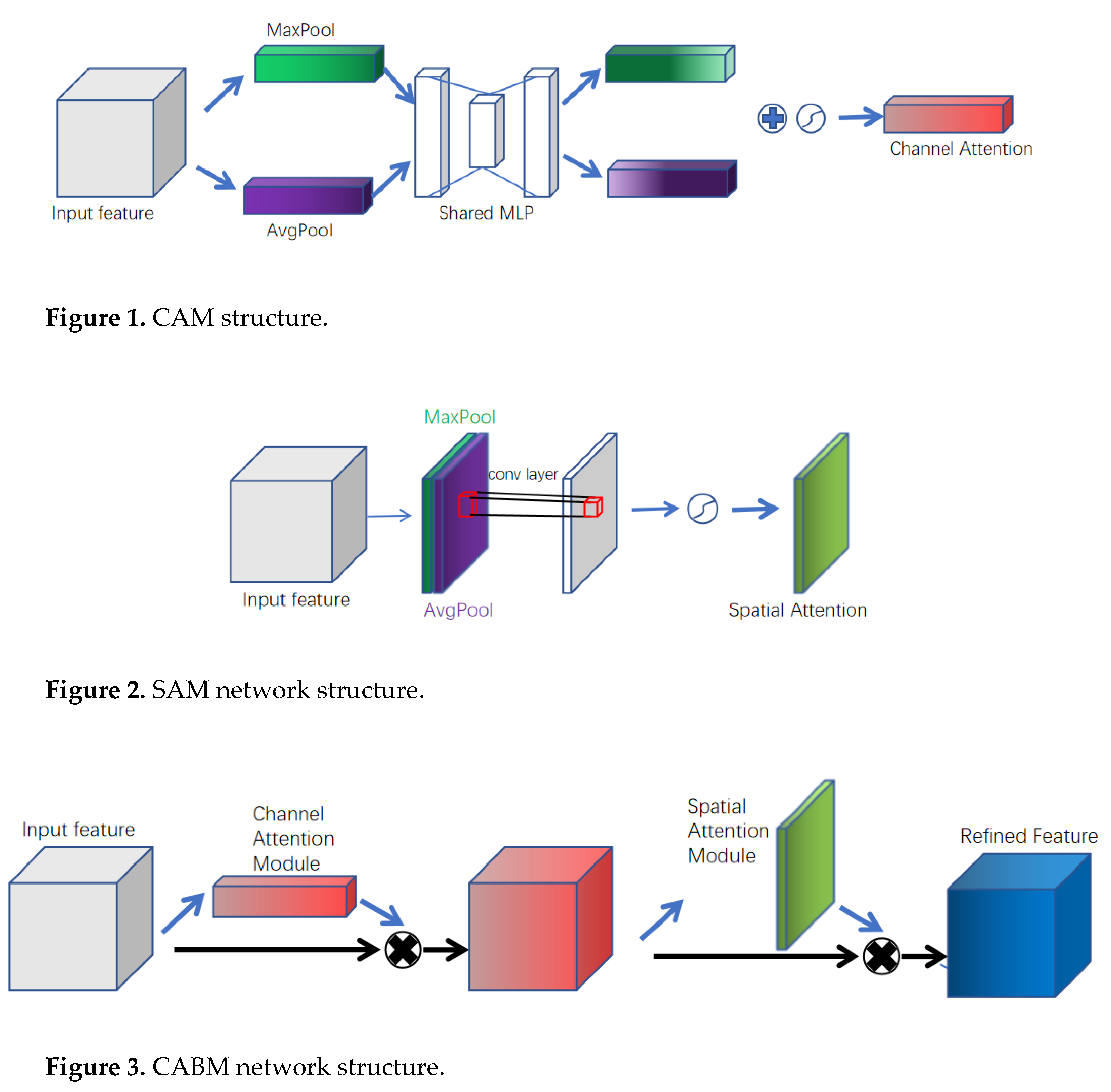
The CBAM contains the Channel Attention Mechanism (Channel Attention Module, CAM) and Spatial Attention Mechanism (Spatial Attention Module, SAM), with two sub-modules, (Figures 1 and 2, respectively). The Channel Attention Mechanism is a one-dimensional vector obtained by compressing a feature map in the spatial dimension. Mean and maximum pooling operations were used to compress the spatial and channel dimensions. The mean and maximum pooling aggregate the spatial information of the feature map, which is then mapped to the weights of each channel through the convolutional layer or fully connected layer. The original features are multiplied with this vector in the channel dimension to obtain the weighted feature map, and the size of the weights reflects the degree of relevance and importance of the features in the layer (channel) for the key information. CBAM contains a spatial attention mechanism and a channel attention mechanism, and the structure is shown in Figure 3. The CBAM is a simple yet effective attention module for feedforward CNNs. The module sequentially infers attention maps along two separate dimensions, channel and spatial, and then multiplies the attention maps with the input feature map for adaptive feature refinement. It can be seamlessly integrated into any CNN architecture with negligible overhead and is end-to-end trainable along with the base CNNs to improve the accuracy of the CNN [25].

Li et al. proposed an improved YOLOv4-based pavement damage detection model. The model improves the saliency of pavement damage by introducing a convolutional block attention module (CBAM) to suppress background noise and explores the influence of the embedding position of the CBAM module in the YOLOv4 model on detection accuracy. The results indicate that embedding CBAM into the neck and head modules can effectively improve the detection accuracy of the YOLOv4 model [26].

Sun et al. proposed an attention-based feature pyramid module (AFPM), which integrates the attention mechanism based on a multi-level feature pyramid network to efficiently and pertinently extract high-level semantic features and low-level spatial structure features, thus improving the accuracy of instance segmentation [27]. According to the above findings, the Convolutional Block Attention Module (CBAM) can independently learn the importance of each channel and space feature, recalibrate the channel and space features, and improve image classification performance [28]. Therefore, in this study, CBAM was added to multiple locations of U²-Net.

2.2.2. SCM-RSU and SC-U²-Net Network

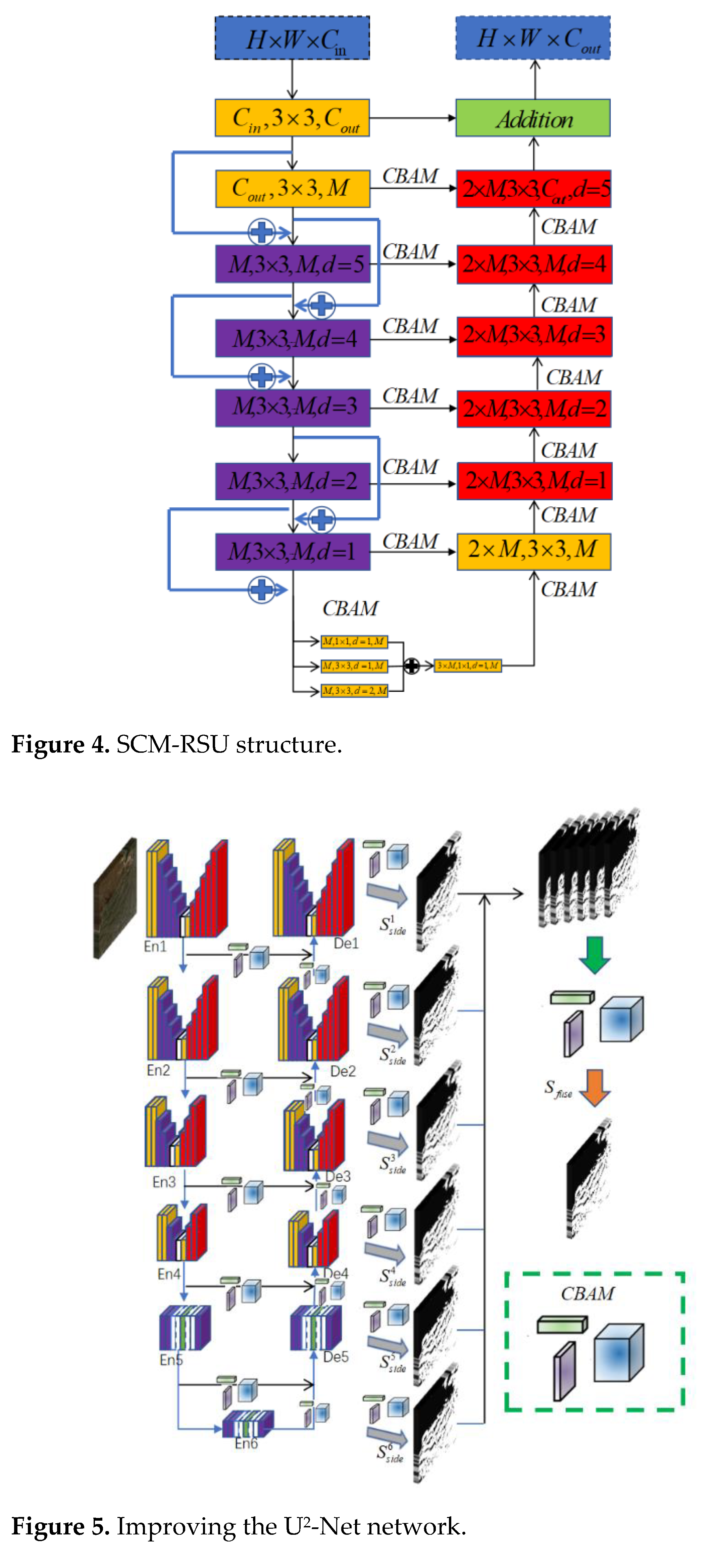
The SC-U²-Net improvement was divided into two parts. First, the SCM-RSU was used instead of the RSU (Figure 4). In the downsampling stage, SCM-RSU used the residual structure, and the output of the upper layer skipped the intermediate convolution as the input of the lower convolution directly to reduce the loss of features in the downsampling process. The U²-Net network used multi-scale expansion convolution only in RSU-4F, which was located in the deep layer of the network, to extract richer features at different scales. The SCM-RSU deep perception module was changed to multi-scale expansion convolution, where the input feature maps were subjected to 1×1 convolution with an expansion factor (d) of 1, 3×3 convolution with a d of 1, and 3×3 expansion with a d of 2, respectively. Subsequently, the outputs of the three convolutions were stitched in the channel dimension, and finally, channel fusion was performed using a 1×1 convolution. In the decoding stage, the output of the same depth encoding and that of the previous decoding depth were processed by the CBAM attention mechanism and inputted.

Secondly, in the overall framework, multiple attention mechanisms were added (Figure 5). The feature map of the encoder output feature map decoder upsampling after using CBAM processing and then input to the corresponding Decoder; the Decoder output feature map enables CBAM processing and then convolution operation to obtain the feature map with channel number 1; each feature map upsampled to the input image. After upsampling each feature map to the size of the input image, stitching was performed to obtain an output with a channel number of 6 and the same size as the original image, and then CBAM was used to process the output. Finally, the output with a channel number of 1 was obtained using 1×1 convolution.

2.3. Sea Ice Image Segmentation Experimental Setup

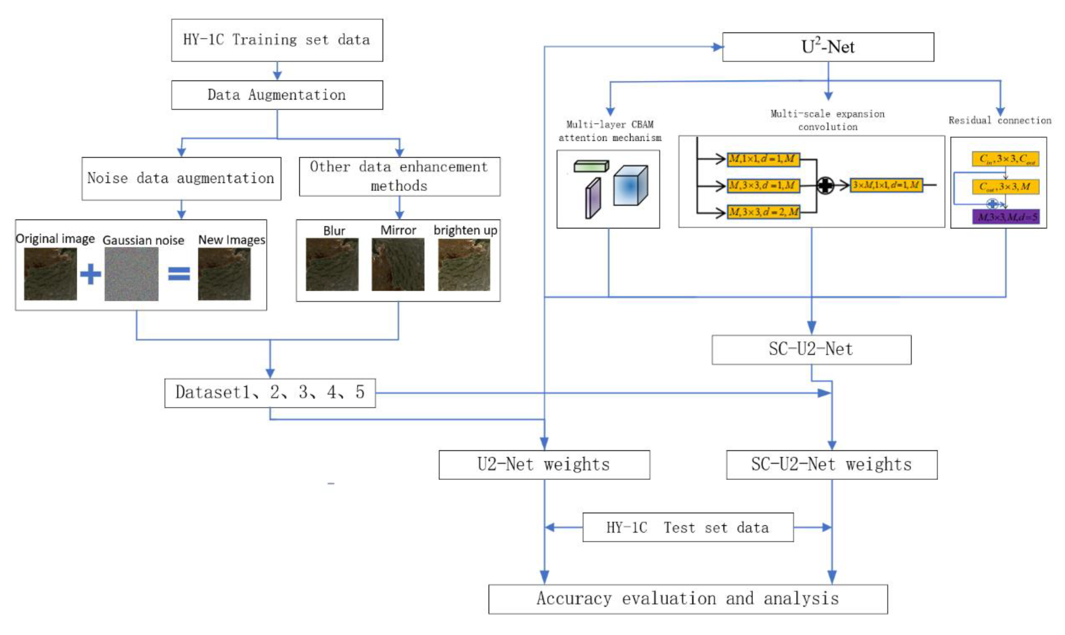
In order to improve the accuracy of sea ice image segmentation, this paper improves two aspects of data augmentation and the U²-Net network structure. In terms of data augmentation, five data sets were constructed using various data augmentation methods (such as noisy data augmentation), and the model weights were obtained by training the U²-Net network with the five data sets respectively, and the accuracy was checked using the test set. In terms of network structure improvement, a multi-layer CBAM attention mechanism and multi-scale expanded convolution were added to U²-Net to enhance the network feature extraction ability, and the accuracy and generalization ability of the improved model were checked using the test set. The SC-U²-Net network model was constructed by adding a multi-layer, CBAM attention mechanism and multi-scale inflation convolution to enhance the network feature extraction ability. The accuracy and generalization ability of the improved model were tested using test data (Figure 6).

Figure 6. Flow chart of sea ice segmentation.

Figure 6. Flow chart of sea ice segmentation.

The initial learning rate was set to 0.001, and this study used the learning rate warmup. The learning rate warmup [29] and cosine annealing [30] were used to combine the learning rate change strategy. The weights of the neural network were randomly initialized at the beginning of training, and the warmup gradually increased the learning rate from low to high to ensure a good convergence of the network. When the gradient descent algorithm was used to optimize the objective function, cosine annealing reduced the learning rate of the cosine function as it approached the global minimum of the loss value, making the model as close to the optimal value as possible. The loss function is a binary cross-entropy loss function (Equation (7)), where

$\stackrel{\wedge }{y}$ is the result of the model prediction sample and $y$ is the sample label.

The loss function of U²-Net is calculated in Equation 8, which contains two parts:

${\displaystyle \sum _{m=1}^M{w}_{side}^{(m)}{l}_{side}^{(m)}}$ represents the sum of the cross-entropy of the output results of different depth Decoder and GT images, and

$w_{fuse}{l}_{fuse}$ is the cross-entropy loss of the final output and GT images after multichannel fusion.

$$Loss=-(y\cdot \log (\stackrel{\wedge }{y})+(1-y)\cdot \log (1-\stackrel{\wedge }{y})$$

(7)

$$L={\displaystyle \sum _{m=1}^M{w}_{side}^{(m)}{l}_{side}^{(m)}+w_{fuse}{l}_{fuse}}$$

(8)

The validation accuracy of the model increased with an increase in epochs, and the model started to converge when the epoch reached 360 when the U²-Net network was trained using training set 1. To balance model accuracy and training efficiency, the epoch was set to 360 in this study. Five test sets were used for training, in which the epochs of training datasets 1 and 2 were set to 360, the epochs of datasets 3, 4, and 5 were set to 90, and the epochs of datasets 3, 4, and 5 were set to 90.

The accuracy evaluation metrics selected in this study are the Intersection over Union (Iou), F1-Score, and recall. If sea ice is called a positive case (Positive), non-sea ice is called a negative case (Negative), and the classifier predicts correctly is noted as True (True) and incorrectly predicts as False (False), and the four basic terms are combined with each other to form the four basic elements of the confusion matrix, true case (TP), false positive case (FP), false negative case (FN), and true negative case (TN), then Iou, F1-Score, Recall are calculated by Equations (9)–(11).

$$IoU=\frac{TP}{TP+FP+FN}$$

(9)

$$F_1=\frac{2TP}{2TP+FN+FP}$$

(10)

$$\mathrm{Re}call=\frac{TP}{TP+FN}$$

(11)

To distinguish the network model from the dataset used for training, the naming rules for the network and model weights were as follows: The U²-Net network was trained using dataset i, and the names of the model weights were obtained as U²-Net-i.

3. Results

3.1. Data Augmentation Experiments

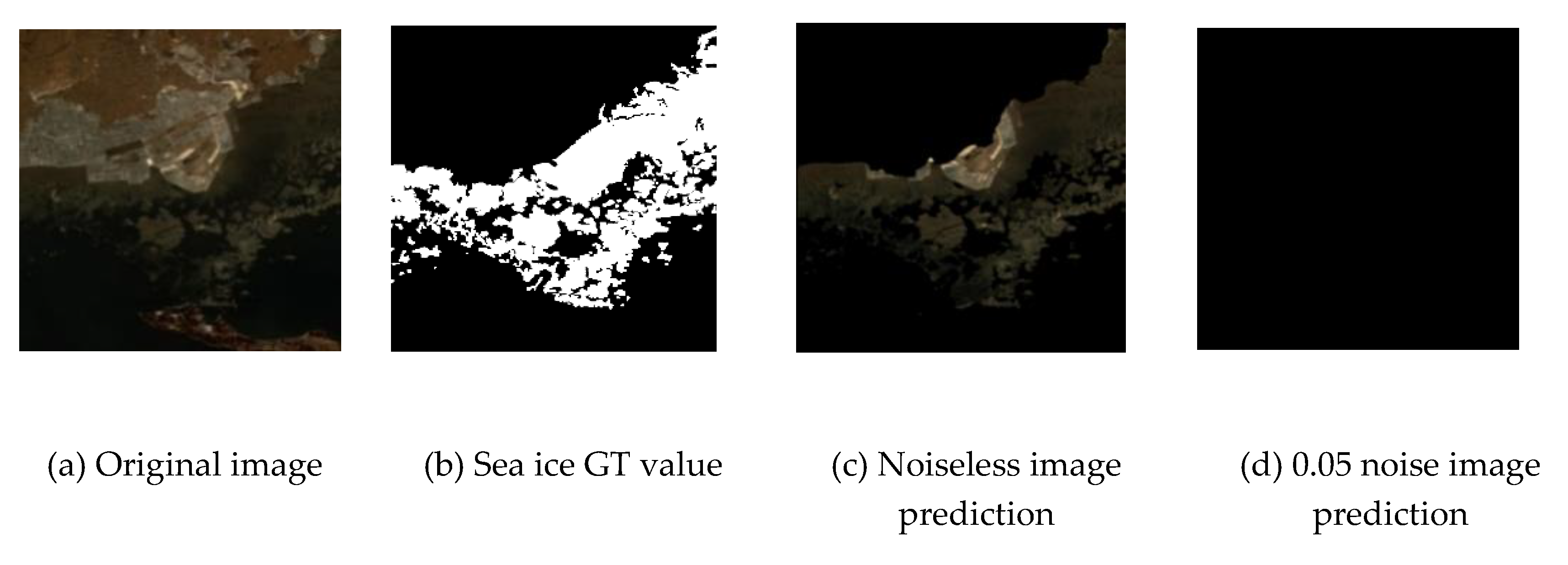
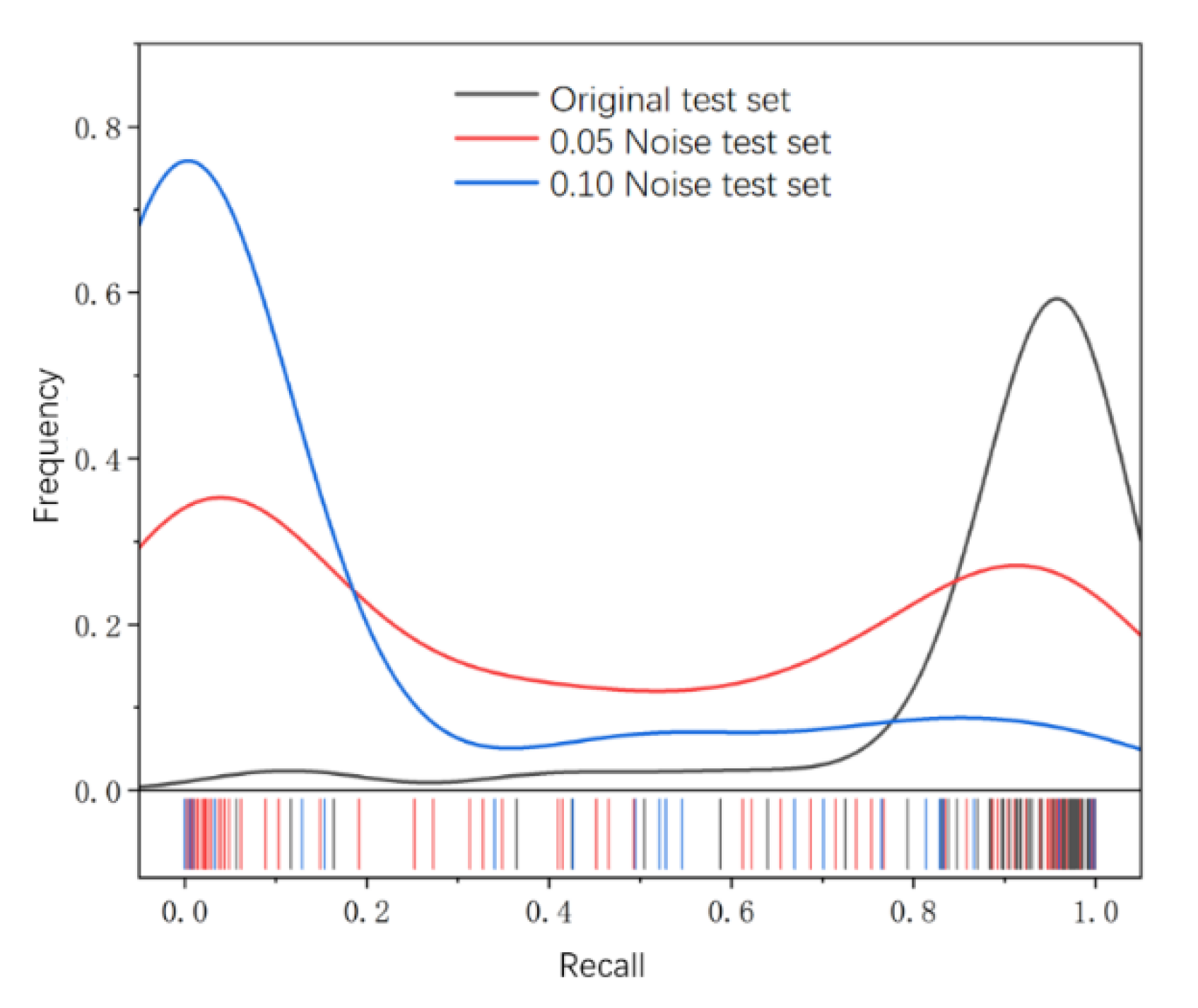
The average cross-merge ratio of U²-Net-1 tested on the test set was 0.842, the average recall was 0.897, and the average F1-Score was 0.889. U²-Net-1 predicted noise-free sea ice images well, but there was overfitting of the network weights, and weak noise interfered with the segmentation, as shown in Figure 7d. The recall distribution curves of U²-Net-1 predicting noise-free images and weakly noisy test set images are shown in Figure 8.

Figure 7. U²-Net-1 predicted noise image.

Figure 7. U²-Net-1 predicted noise image.

Figure 8. U²-Net-1 recall distribution probability curve.

Figure 8. U²-Net-1 recall distribution probability curve.

To further study the effect of noise, we trained U²-Net using different training sets to obtain the corresponding model weights (U²-Net-1 was the weight obtained by training U²-Net on training set 1). 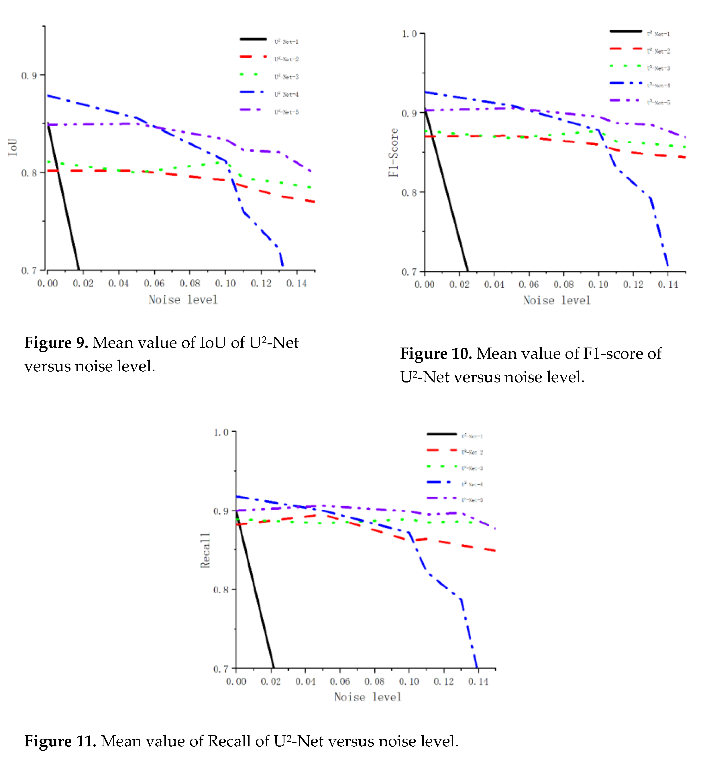We performed a segmentation of the test set containing different noise levels using U²-net trained from different training sets.The average IoU, average recall, and average F1-Score of the test set with different noise levels were counted (Table 2). The curves of average IoU, average recall average F1-Score with noise level of the test set were made according to Table 2, as shown in Figure 9, Figure 10 and Figure 11 respectively.

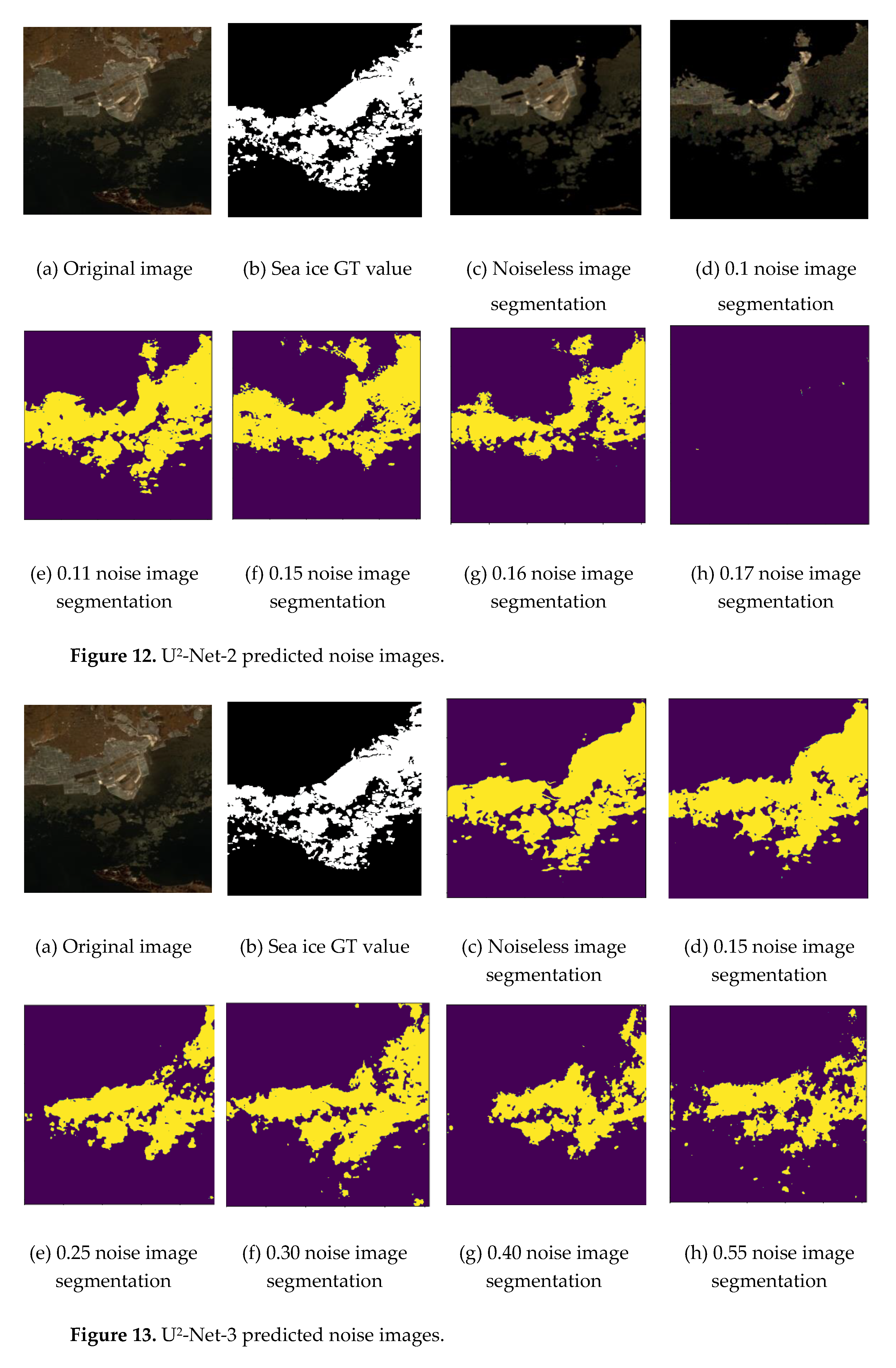
Figures 12 and 13 show the results of U²-Net-2 and model U²-Net-3 predicting different levels of test set. Model 2 could predict images with low noise, but the predicted noise limit was approximately 0.15; U²-Net-3 had a stronger generalization ability than model U²-Net-2 and was able to segment images with more severe noise pollution.

To further verify the usefulness of multiple data augmentation methods, the transformations (e.g., rotation and mirroring) were performed on the test set simultaneously to obtain a test set with different geometric and radiometric characteristics from the original test set in this study. The experimental accuracies are shown in Table 3 using the transformed test sets for U²-Net-3, U²-Net-4, and U²-Net-5.

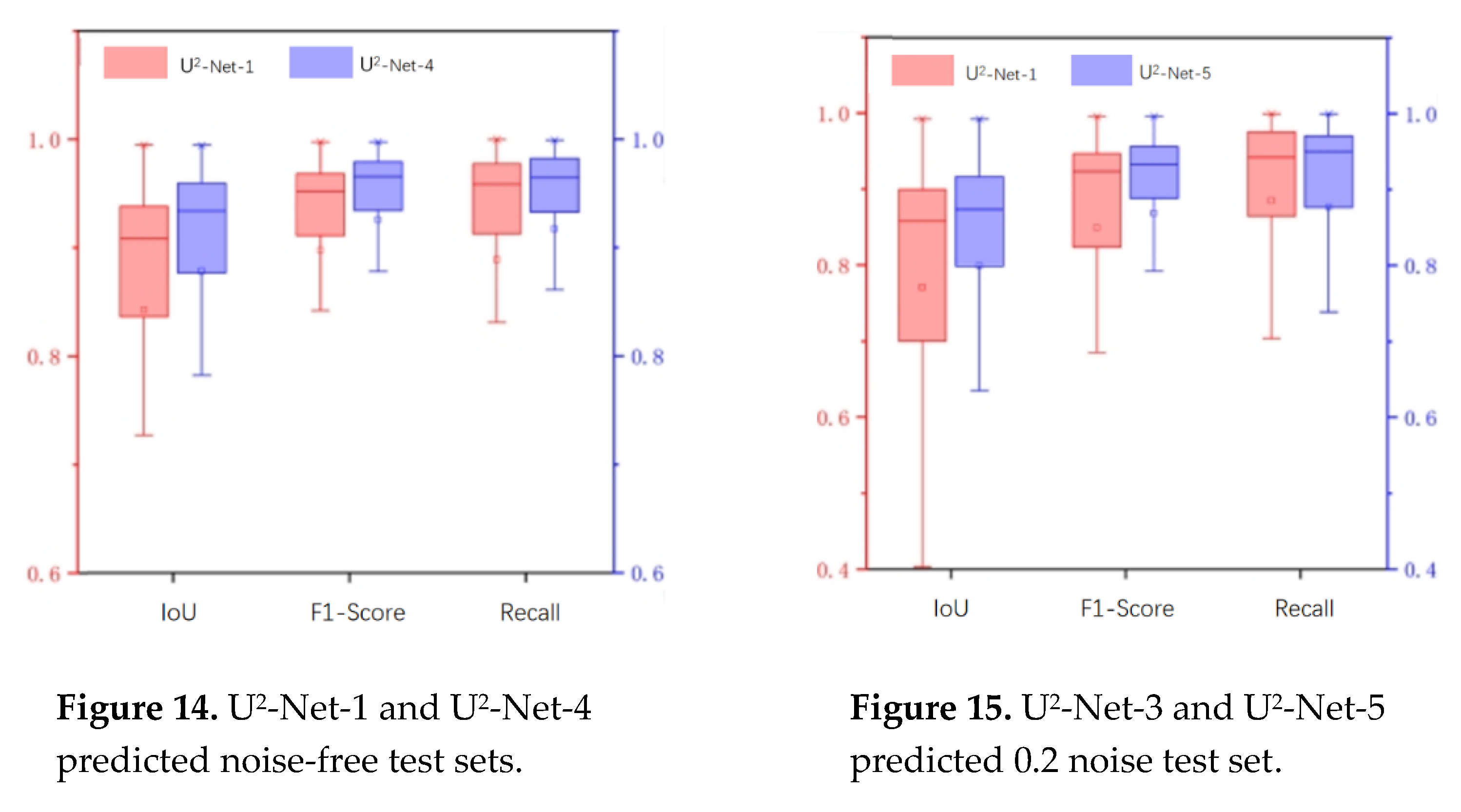
The accuracy evaluation indices of U²-Net-4 were higher than those of U²-Net-1 when predicting the noiseless test set (Figure 14). The accuracy evaluation indices of U²-Net-5 were higher than those of U²-Net-3 when predicting the test set with 0.2 noise level (Figure 15).

3.2. SC-U²-Net Network

The SC-U²-Net-1 and U2-Net-1 network was trained using the same dataset(Training dataset 1). The accuracies of SC-U²-Net-1 and U²-Net-1 were tested using the test set, and the accuracy of SC-U²-Net-1 and U²-Net-1 tests are shown in Table 4.

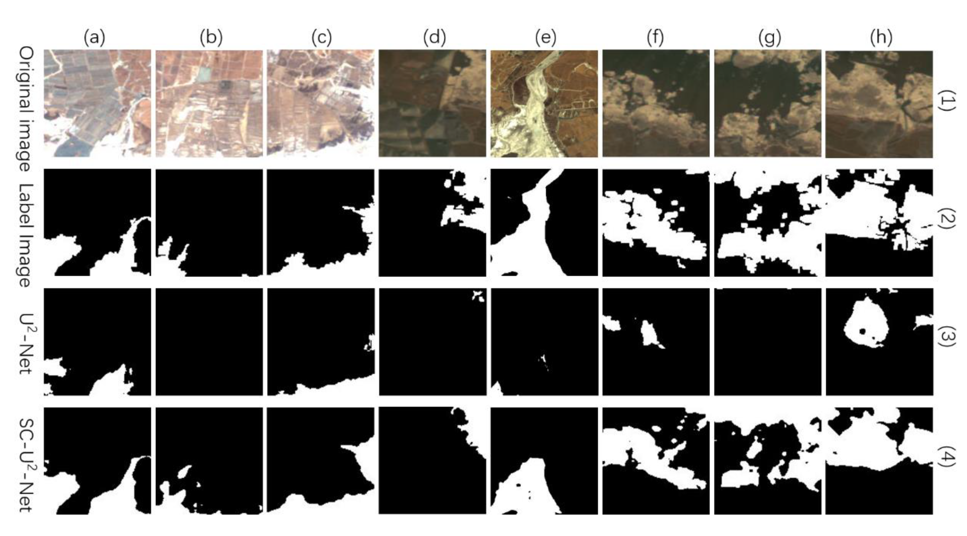
Figure 16 shows some experimental results, where figures (a) to (h) show the sea ice images of different regions, and (1) to (4) show the original image, labeled image, U²-Net segmentation result, and SC-U²-Net segmentation result, respectively. U²-Net was less effective in segmenting some sea ice, such as the broken ice area at the land edge. SC-U²-Net performed better and could extract the outline and some details of sea ice as shown in (a) of Figure 16.

Figure 16. Comparison of SC-U²-Net and U²-Net segmentation results.

Figure 16. Comparison of SC-U²-Net and U²-Net segmentation results.

The accuracy of SC-U²-Net-5 was examined using an extended test set (1500 images) and compared to U²-Net-5. The IoU, F1-Score and recall of U²-Net-5 and SC-U²-Net-5 on the extended test set are shown in Table 5.

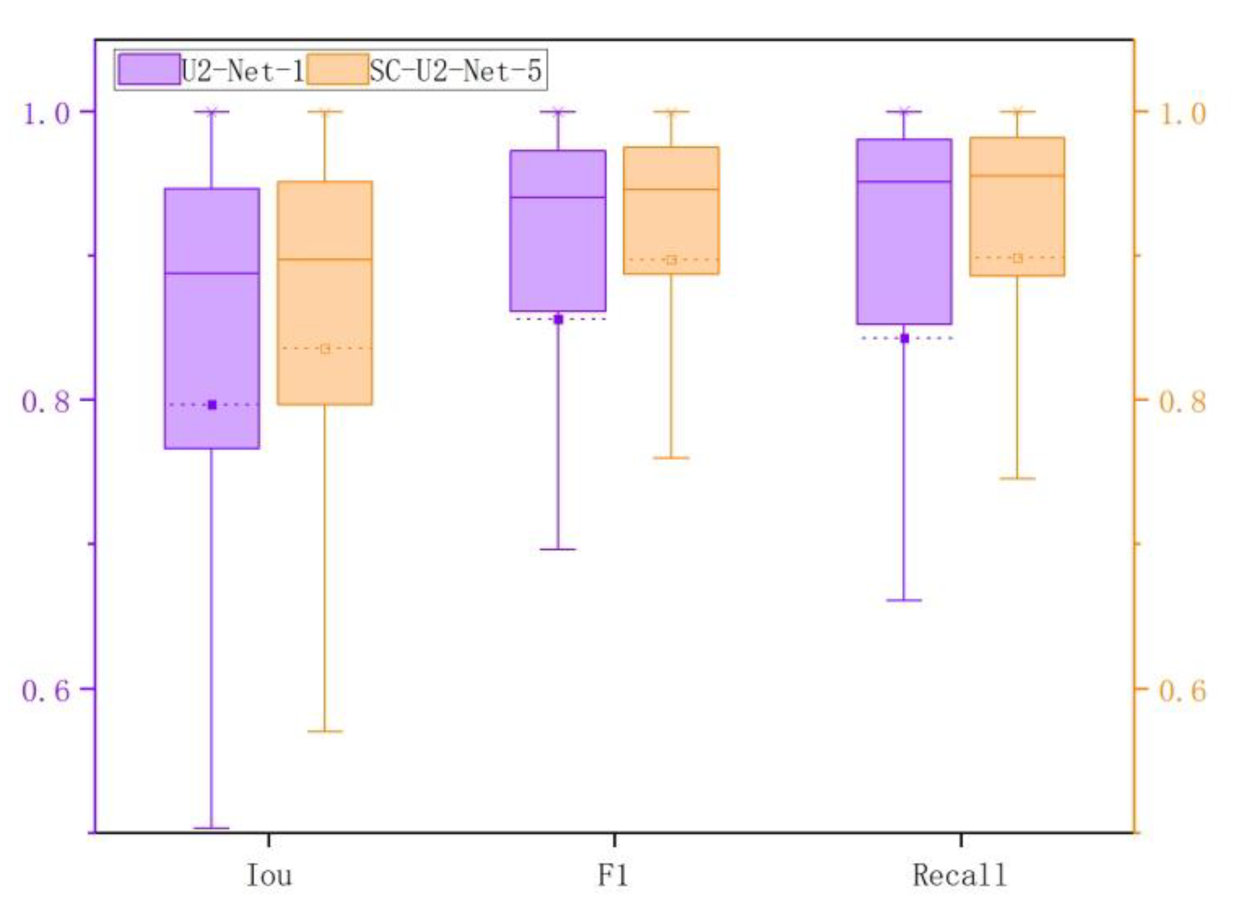
Using the transformed test sets to test U²-Net-1 and SC-U²-Net-5, the statistics of IoU, F1-Score, and recall per image for each test set were calculated (Table 3; Figure 17). SC-U²-Net-5 had a much better segmentation effect than U²-Net-1 on each test set (Table 6). The results in Table 6 show that the simultaneous use of data augmentation and network improvements can improve the accuracy and generalization of the model.

Figure 17. U²-Net-1 and SC-U²-Net-5 accuracy rating box line diagram.

Figure 17. U²-Net-1 and SC-U²-Net-5 accuracy rating box line diagram.

4. Discussion

4.1. Data Augmentation Experiments

U²-Net-1 is very sensitive to noise, and the low intensity of Gaussian noise makes it difficult for Model 1 to achieve the semantic segmentation of sea ice images. When the test set did not contain noise, the recall was mainly concentrated at 0.8–1.0, and when the noise level was 0.05, the recall was bimodal (partly concentrated in 0.8-1.0 and partly concentrated in 0-0.2, which indicates that the weak noise interfered with the prediction of the model and can only achieve more accurate segmentation for a part of the images, while the segmentation accuracy of another part of the images was close to 0; the noise level was 0.1, and the recall of all predicted images was concentrated around 0. This shows that noise reduces the accuracy of U²-net semantic segmentation.

To enhance the generalization ability of U²-net, different levels of noise are added to the training set for augmentation. The training training set after adding noise has a minimal loss of accuracy, but the generalization ability of the model is enhanced.The comparative analysis led to the following conclusions: first, for the noise-free dataset, U²-Net-1 had the best segmentation effect; second, in terms of noise resistance, U²-Net-3 was better than U²-Net-2, which was better than U²-Net-1. Especially in U²-Net-1 (no noise was added to the training set), the noise made the prediction accu-racy decay rapidly. Third, in terms of generalization, the model with the noisy training set resisted the interference of noise; the richer the noise level was, the stronger its noise resistance was.U²-Net-2 could predict images with low noise, but the predicted noise limit was approximately 0.15; U²-Net-3 had a stronger generalization ability than model U²-Net-2 and was able to segment images with more severe noise pollution.

U-Net-4 was obtained using training set 4, and the accuracy evaluation indices of U²-Net-4 were higher than those of U²-Net-1 when predicting the noiseless test set. U2-Net-5 was obtained by training U²-Net network with data set 5, and the accuracy evaluation indices of U²-Net-5 were higher than those of U²-Net-3 when predicting the test set with 0.2 noise level. multiple data augmentation methods not only improves the model's ability to cope with complex scene transformations but also improves the accuracy of semantic segmentation. We also constructed additional test sets with affine transformation, mirror flip and blurring. The augmented training set images in the training of U²-Net-4 and U²-Net-5 enabled the network to learn multi-perspective and multi-scale semantic features, making U²-Net-4 and U²-Net-5 cope well with complex scenarios. We also constructed additional test sets with affine transformation, mirror flip and blurring. U²-Net-4 and U²-Net-5 performed better on these test sets.

Data augmentation experiments showed that U²-Net-1, which was trained using only the original data, was very sensitive to noise and that adding a small perturbation to the grayscale values of the original images caused U²-Net-1 to fail. This was because the number of images in the training set was small, and the scene was single, which results in U²-Net overfitting. Noisy data augmentation expanded the sample size and improved the generalization ability of the model. U²-Net-2 and U²-Net-3 showed a more stable prediction ability when predicting images with noise.The semantic segmentation accuracies of U²-Net-4 and U²-Net-5 were close to that of U²-Net-3 tested on the test set, and the new test set was obtained by subjecting the test set to affine transformation, mirror flipping, and blurring. The semantic segmentation accuracy of U²-Net-4 and U²-Net-5 was much better than that of U²-Net-3 on the new test set because the training sets of U²-Net-4 and U²-Net-5 used a variety of data augmentation in the training. The augmented training set images in the training of U²-Net-4 and U²-Net-5 enabled the network to learn multi-perspective and multi-scale semantic features, making U -Net-4 and U -Net-5 cope well with complex scenarios.

4.2. SC-U²-Net Network

In the comparison experiments of U²-Net and SC-U²-Net, we use the same training set to train U²-Net and SC-U²-Net, so as to exclude the accuracy improvement brought by the increase of data set, and the experiments show that Using the same training and test sets, the IoU, F1-Score, and recall of SC-U²-Net were higher than those of U²-Net. SC-U²-Net is more effective for sea ice segmentation on remote sensing images. We also compare U²-Net-1 (U²-Net trained without data augmentation) and SC-U²-Net-5 (SC-U²-Net trained with data augmentation), and the results show that the simultaneous use of data augmentation and network improvement can improve the accuracy and generalization of the model. SC-U²-Net was able to segment the narrowly shaped sea ice with a smaller area, and the segmentation results are basically consistent with the labeled images. U²-Net is effective in segmenting sea ice over a large area on the sea surface, while narrowly shaped sea ice extending into the land interior is ignored. Compared with U²-Net, the improved SC-U²-Net was able to pay more attention to the details of the target and segmented the discontinuous sea ice better.

5. Conclusions

Based on the U²-Net semantic segmentation network, this study expanded the training set using a data augmentation method and investigated the effect of data augmentation on the accuracy and generalization ability of U²-Net. In the case of poor segmentation of some sea ice images, the SC-U²-Net network was constructed by adding a multi-scale, inflation convolution and multi-layer CBAM attention mechanism on top of U²-Net, and its accuracy was compared with that of the U²-Net network. The study concluded the following: (1) U²-Net could segment the original test set images well, but the model generalization was poor. (2) The multilevel Gaussian noise data enhancement scheme designed in this study improved the noise interference resistance of the network, considered the generalization performance and accuracy of the model, and achieved more accurate segmentation of images with different degrees of noise pollution. (3) In SC-U²-Net, the residual structure reduced the loss of features during downsampling, multi-scale inflation convolution increased the perceptual field of deep convolution, and the multi-layer CBAM attention mechanism improved the recognition ability of the network for local features. SC-U²-Net had a higher average IoU, average F1-Score, and average recall rate than U²-Net for each test set, especially for fragmented sea ice regions.

The limitations of the experiments were as follows:(1) From the experimental data, the amount of training and test data were relatively small, which affects the reliability of the network training effect and test accuracy. (2) In the experimental setup, only U²-Net and SC-U²-Net were compared, and the other networks were not used as references in the accuracy assessment. (3) The experimental results indicated that, although both data augmentation and network improvement could improve the accuracy of semantic segmentation, the improvement was not substantial enough.

References

- Liu, M. Research on the Sea Ice Classification and Thickness Detection with High-Resolution and Polarimetric SAR Data. College of Information and Control Engineering China University of Petroleum (EastChina), 2016.
- Liang, J. Maritime Strategic Game in Arctic Region: China and India. S. Asian Stud. Q. 2019, 24–33. [Google Scholar]
- Cheng, X.; Chen, Z.; Hui, F. Current Status and Outlook of Space-Based Remote Sensing Observation in Polar Regions of China. Sci. Technol. Foresight 2022, 1, 183–197. [Google Scholar]
- Wang, L. Research on Sea Ice Inversion Algorithm Based on Satellite Remote Sensing Data. Nanjing University of Information Engineering, 2021.
- Li, Y. Research on Sea Ice Detection Method Based on the Decomposition of Mixed Pixels; Wuhan University, 2020.
- Li, P. Combining Active Learning and Semi-supervised Learning for Sea Ice Image Classification; Shanghai Ocean University, 2018.
- Han, Y.; Li, J.; Zhang, Y.; Hong, Z. Hyperspectral Sea Ice Detection Using Improved Similarity Metric. Remote Sens. Inf. 2018, 33, 76–85. [Google Scholar]
- Zhou, J.; Lu, P.; Wang, Q.; Xie, F.; Li, R. Research on Automatic Detection Algorithm Based on Video Image Acquisition for Ice Surface Features. Hydro Science Cold Zone Eng. 2021, 4, 60–65. [Google Scholar]
- Yu, Z. Sea Ice Classification of Remote Sensing Image Based on Neighborhood Relationships; CUPB (East China),2019.
- Dowden, B.; De Silva, O.; Huang, W.; Oldford, D. Sea Ice Classification via Deep Neural Network Semantic Segmentation. I.E.E.E. Sens. J. 2021, 21(10), 11879–11888. [Google Scholar] [CrossRef]
- Han, Y.; Cui, P.; Zhang, Y.; Zhou, R.; Yang, S.; Wang, J. Remote Sensing Sea Ice Image Classification Based on Multilevel Feature Fusion and Residual Network. Math. Probl. Eng. 2021, 2021, 1–10. [Google Scholar] [CrossRef]
- Shi, Q. Homologous and Heterologous Remote Sensing Sea Ice Classification Based on Deep Learning; Shanghai Ocean University, 2022.
- Fang, Y. Research on Sea Ice Area Identification Based on MODIS Satellite Remote Sensing Images; Qingdao University of Science and Technology, 2021.
- Cui, Y.; Zou, B.; Han, Z.; Shi, L.; Liu, S. Application of Convolutional Neural Networks in Satellite Remote Sensing Sea Ice Image Classification: A Case Study of Sea Ice in the Bohai Sea. Acta Oceanol. Sin. 2020, 42, 100–109. [Google Scholar] [CrossRef]
- Han, Y.; Gao, Y.; Zhang, Y.; Wang, J.; Yang, S. Hyperspectral Sea Ice Image Classification Based on the Spectral-Spatial-Joint Feature with Deep Learning. Remote Sens. 2019, 11(18), 2170. [Google Scholar] [CrossRef]
- Han, Y.; Liu, Y.; Hong, Z.; Zhang, Y.; Yang, S.; Wang, J. Sea Ice Image Classification Based on Heterogeneous Data Fusion and Deep Learning. Remote Sens. 2021, 13(4), 592. [Google Scholar] [CrossRef]
- Zhang, T.; Yang, Y.; Shokr, M.; Mi, C.; Li, X.; Cheng, X.; Hui, F. Deep Learning Based Sea Ice Classification with Gaofen-3 Fully Polarimetric SAR Data. Remote Sens. 2019, 13(8), 1452. [Google Scholar] [CrossRef]
- Wen, C.; Zhai, M.; Lei, R.; Xie, T.; Zhu, J. Automated Identification of Landfast Sea Ice in the Laptev Sea from the True-Color MODIS Images Using the Method of Deep Learning. Remote Sens. 2023, 15(6), 1610. [Google Scholar] [CrossRef]
- Liu, Z.; Zhang, S.; Liu, Y.; Luo, C.; Li, M. Data Augmentation Method Based on Image Gradient. J. Appl. Sci. 2023, 39, 302–311. [Google Scholar]
- Huang, Z.; Liu, X.; Shi, y.; Lin, C. Small Object Detection in Road Science Base on Data Augmenttation. Journeal Wuhan Univ. Technol. 2022, 44, 79–87. [Google Scholar]
- Yang, Z.; Yang, Y.; Cang, S.; Li, Y.; H.; Y.; Zhang, F.; Wu, G. Data Augmentation Method of Ship Remote Sensing Images Based on GAN. Appl. Sci. Technol. 2022, 49, 8.
- Lin, C.; Shan, C.; Zhao, G.; Yang, Z.; Peng, J.; Chen, S.; Huang, R.; Li, Z.; Yi, X.; Du, J.; Li, S.; Luo, H.; Fan, X.; Chen, B. Review of Image Data Augmentation in Computer Vision. J. Front. Comput. Sci. Technol. 2021, 15, 583–611. [Google Scholar]
- Lee, D.-U.; Villasenor, J. D.; Luk, W.; Leong, P. H. W. A Hardware Gaussian Noise Generator Using the Box-Muller Method and Its Error Analysis. In I.E.E.E. Trans. Comput. 2006, 55(6), 659–671. [Google Scholar] [CrossRef]
- Qin, X.; Zhang, Z.; Huang, C.; Dehghan, M.; Zaiane, O. R.; Jagersand, M. U2-Net: Going Deeper with Nested U-Structure for Salient Object Detection. Pattern Recognit. 2020, 106, 107404. [Google Scholar] [CrossRef]
- Woo, S.; Park, J.; Lee, J.; Kweon, I. S. Cbam: Convolutional Block Attention Module. In Proceedings of the European Conference on Computer Vision (ECCV); 2018; pp. 3–19. [Google Scholar] [CrossRef]
- Li, L.; Fang, B.; Zhu, J. Performance Analysis of the YOLOv4 Algorithm for Pavement Damage Image Detection with Different Embedding Positions of CBAM Modules. Appl. Sci. 2022, 12(19), 10180. [Google Scholar] [CrossRef]
- Sun, Y.; Gao, W.; Pan, S.; Zhao, T.; Peng, Y. An Efficient Module for Instance Segmentation Based on Multi-level Features and Attention Mechanisms. Appl. Sci. 2021, 11(3), 968. [Google Scholar] [CrossRef]
- Zhang, L.; Duan, L. Cross-Scenario Transfer Diagnosis of Reciprocating Compressor Based on CBAM and ResNet. J. Intell. Fuzzy Syst. 2022, 43(5), 5929–5943. [Google Scholar] [CrossRef]
- Xiong, R.; Yang, Y.; Di He; Zheng, K.; Zheng, S.; Xing, C.; Zhang, H.; Lan, Y.; Wang, L.; Liu, T. On Layer Normalization in the Transformer Architecture. ICML. 2020.
- Loshchilov, I.; Hutter, F. SGDR: Stochastic Gradient Descent with Warm Restarts. ICLR 2017, 1–16. [Google Scholar]