You are currently viewing a beta version of our website. If you spot anything unusual, kindly let us know.

Preprint

Article

Bootstrap Approach for Principal Component Analysis Method; Cases studies

Altmetrics

Downloads

631

Views

Comments

This version is not peer-reviewed

Abstract

Analyzing big data poses a great challenge for numerous researchers to explore the data structure. Dimension reduction methods can be used to reduce data dimensionality, taking it from occupying a high-dimensional space to existing in a lower-dimensional space while retaining as much information as possible. Principal Component Analysis is one of the most popular used to reduce the dimensional space. The bootstrap sample is obtained by randomly sampling n times with replacement from the original sample, the method provides easy tool to understand the interactive component and develop the process. There are not enough researches discussed the stability of PCA method using bootstrap method. In this paper, the bootstrap method is used to analyze the stability of PCA results and to estimate the number of PCA in efficient way. The method is used to estimate the number of PCA that needed to classify the data set, and the effectiveness of the discussed techniques is demonstrated through real data sets.

Keywords:

Subject: Computer Science and Mathematics - Probability and Statistics

1. Introduction

Data visualizing are receiving more attention since they are easier to understand and summing up data. Dealing with big data poses a challenge with "curse of dimension" and computation capacity among other issues [1]. Dimension reduction methods project the data dimensionality into a lower-dimensional space while retaining as much information as possible. These methods reduce the data storage and computation time, besides, overcome the complexity of the model. In recent decades, scientists have used various methods of machine learning (ML) to detect patterns and determine the intrinsic dimensions of big data to generate actionable insights, this could be handled by a range of dimension reduction methods. The set of techniques available for dimensionality reduction can be divided into techniques for supervised and unsupervised learning applications. Unsupervised methods aim to detect similarities and differences inside a dataset.

Principal component analysis (PCA) is one of the most popular dimension reduction methods [2], it is also known as unsupervised method. The main purpose of PCA is to reduce the dimensionality of a data set consisting of a large number of interrelated variables while retaining as much as possible of the variation present in the data set. PCA was briefly mentioned by Fisher and Mackenzie [3] as being more suitable than analysis of variance for the modelling of response data.

Fisher and Mackenzie [3] also outlined the NIPALS algorithm, later rediscovered by Wold [4]. Hotelling [5] further developed PCA to its present stage. Since then, the utility of PCA has been rediscovered in many diverse scientific fields, resulting in, amongst other things, an abundance of redundant terminology. Rao [6] paper is remarkable for the large number of new ideas concerning uses, interpretations and extensions of PCA that it introduced. Various fields apply PCA in applications such as: face recognition, handprint recognition, and mobile robotics. More applications are discussed in [7].

The bootstrap method was introduced by Efron [8]. It is a resampling technique for estimating the distribution of statistics based on independent observations, and then developed to work with other statistical inference. It is used for assigning the measures of accuracy of the sample estimate, especially the standard error. The bootstrap sample is obtained by randomly sampling n times with replacement from the original sample. In this paper, the bootstrap method is used to analyze the stability of PCA results and to estimate the number of PCA in efficient way. The method is used to estimate the number of PCA that needed to classify the data set. For a good introduction to the bootstrap method, see[9]. The bootstrap method can be applied to with a lot of applications, such as tests, regression, and confidence intervals. And used as a useful statistical tool with clustering and mixture models [10,11]. Binhimd and Coolen [12] introduced a new bootstrap method based on nonparametric predictive inference. It is called NPI-B. They compared between (NPI-B) and Efron's classical bootstrap method (Ef-B), then applied (NPI-B) for reproducibility of some statistical tests. Binhimd and Almalki [13] discussed the comparison between Efron's bootstrap and smoothed Efron's bootstrap using different method. Some literatures discussed the work of bootstrapping principal component analysis [14, 15,16].

Practically, one needs to decide the number of components that need to be retained, which means measuring the stability of components or variables. In terms of statistical modelling, stability could be demanded that a data set drawn from the same underlying distribution should give rise to more or less the same parameter. It means that a meaningful valid parameter (component) should not disappear easily if the data set is changed in a non-essential way [17]. Some of stability rules depend on computationally intensive, such as cross validation, bootstrap or jackknife. In the literatures, bootstrap used to estimate the confidence region for differentiable function of the covariance matrix of the original data, this is done after implementing PCA on the considered data. Another stability criterion, one based on a risk function which is known a distance between orthogonal projectors. The aim of this paper to study the stability of PCA method in such a way to improve the process of existing method and the effectiveness of the discussed techniques is demonstrated through a simulation study and real data sets.

2. Materials and Methods

This section provides a brief overview of the algorithms and procedures that will be used in the paper.

2.1. Principal Component Analysis

Principal component analysis (PCA) is a dimension reduction method that projects the data with high dimensional space into a lower-dimensional sub-space. The new data can then be more easily visualized and analyzed, while retaining as much as possible of the data’s variation. It has applications in various fields, such as face recognition and image compression, it is a common technique for finding patterns in high-dimensional data.

Hence, let

X = {(x_{1}, \dots, x_{D})}^{T}

be a random vector that has a probability density function

f (x)

from a multivariate Gaussian distribution with mean and variance denoted by

μ

and

Σ

, respectively. Assume that a sample of size

N

is drawn from the random vector

X

, yielding data

Z = (x_{1}, \dots, x_{N}) \in R^{D}

, which is N independent and identically distributed (iid) units. The matrix Z has the following structure:

Z = [\begin{matrix} x_{11} & x_{12} & x_{13} & \dots & x_{1 j} & \dots & x_{1 D} \\ x_{21} & x_{22} & x_{23} & \dots & x_{2 j} & \dots & x_{2 D} \\ x_{31} & x_{32} & x_{33} & \dots & x_{3 j} & \dots & x_{3 D} \\ ⋮ & ⋮ & ⋮ & ⋮ & ⋮ & ⋮ & ⋮ \\ x_{N 1} & x_{N 2} & x_{N 3} & \dots & x_{N j} & \dots & x_{N D} \end{matrix}]

(1)

The principal component analysis (PCA) method reduces a large number of associated variables into a manageable number of main components, which are independent linear combinations of those variables.

The main idea of PCA is to illustrate the variation that appears in a dataset that has correlated variable,

X^{T} = (x_{1}, \dots, x_{D})

, then the new dataset of uncorrelated variables

Y^{T} = (y_{1}, \dots, y_{D})

, where each of

y_{i s}

a linear combination of X. The variables in the new data are the principal components, where, the first principal component of the observation,

y_{1}

, is the linear combination:

y_{1} = a_{11} x_{1} + a_{12} x_{2} + \dots + a_{1 D} x_{D}

(2)

Whose sample variance is greatest among all such linear combinations. Because the variance of

y_{1}

can be increased without limit simply by increasing the coefficients

a_{1} = (a_{11}, a_{12}, \dots, a_{1 D})

, a restriction must be placed on these coefficients. As we shall see later, a sensible constraint is to require that the written

a_{1}^{⊺} a_{1} = 1

. The sample variance of

y_{1}

that is a linear function of the

x

variables is given by

a_{1}^{⊺} {S a}_{1}

, where

S

is the

D \times D

sample covariance matrix of the

x

variables. To maximise a function of several variables subject to one or more constraints, the method of

L a g r a n g e m u l t i p l i e r s

is used.

The second principal component,

y_{2}

, is defined to be the linear combination:

y_{2} = a_{21} x_{1} + a_{22} x_{2} + \dots + a_{2 D} x_{D}

(3)

i.e.,

y_{2} = a_{2} x

, where

a_{2} = (a_{21}, a_{22}, \dots, a_{2 D})

and x =

(x_{1}, x_{2}, \dots, x_{D})

that has the greatest variance subject to the following two conditions:

a_{2}^{⊺} a_{2} = 1, a_{2}^{⊺} a_{1} = 0 .

(4)

Usually, the total sum of eigenvalues that are obtained from a covariance matrix is equal to the total sum of variance of each variable.

2.2. Bootstrap

The bootstrap's primary tenet is that, in some circumstances, it is preferable to draw conclusions about a population parameter only from the available data, without making any assumptions about underlying distributions. Compared to traditional inferences, bootstrap approaches can often be considerably more correct. This method was developed to work with different statistical inferences, such as confidence intervals, hypothesis tests, and regression, it is good technique if the sample size is small. The basic method here depends on drawing B random samples of size n with replacement from the original sample, and then calculating the statistic of interest to estimate the sampling distribution and work with the required statistical inference. The issue with the method is that each time we gather a sample, we can receive somewhat different findings. The standard deviation of a point estimate for repeated population samplings theoretically may be quite high, which could bias the estimate.

2.3. Principal Components Analysis with bootstrap confidence interval

The extent to which the estimator is likely to diverge from the parameter must be determined in order to build a confidence interval for the parameter. The main premise behind the bootstrap is to assess how much the estimate swings when it is calculated using resampled versions of the original data.

2.4. Approaches using bootstrap

The bootstrap sample is drawn at random from the original, size N sample with replacement. Construct the bootstrap confidence interval:

The maximum eigenvalue $λ_{i}$ can be found by repeatedly resampling dataset of (B) times. Using the resampled dataset I's covariance matrices.
The difference between the true and bootstrap eigenvalues (d) should be calculated.
A 0.025 percentile and a b=0.975 percentile of d are needed to calculate the confidence interval 95%. The appropriate confidence interval is ( $λ$ true-b, $λ$ true+a).

3. Results

This section explains the implementation of bootstrap method in PCA on the selected data, Protein and Chemical data sets. The section offering a discussion across the following subsections: Section 3.1 presents the results of Protein data; Section 3.2 presents the results of Chemical data.

3.1. Protein data

Protein consumption data consists of 25 rows of observations and 11 variables, the data is collected from 25 European countries for 9 kinds (groups) of foods Gabriel (1981). As first step, the PCA is implemented on this data to insight the data structure and conduct its variability, result is shown in Figure 1. It presents that 91% of the total variance is explained by five components, with PC1 explaining 44.5% of the total variance, and PC2 explaining 18.2% of the total variance. PC3 further explains 12.5% of the total variance, PC4 and PC5 explaining 10.6% and 5.2%, respectively, of the total variance. This offers a perspective on these components’ comparative relationships to the dataset, with just five PCs explaining 91.43% of the total variance. To evaluate the relationship between the multiple variables and the relevant PCs, Table 1 illustrates the squared factor loading for each variable, the total percentage of the variance that can be explained by the two components is around 62.7%. Consider the variables Red_Meat, White_Meat, Eggs, Milk, Fish, Cereal, Starch, Nuts and Fruits_Vegetables, we shall represent them by

X_{1}, X_{2}, X_{3}, X_{4}, X_{5}, X_{6}, X_{7}, X_{8}, X_{9}

, respectively. As illustration in Eq. (5) and Eq. (6), one can infer that highest contributing variables in PC1 are Cereal and Nuts while Eggs provides the highest negative level of contribution. In PC2, the highest contributing variables are Fish and Fruits_Vegetables while Eggs provides a low negative level of contribution.

P C 1 = - 0.303 X_{1} - 0.311 X_{2} - 0.427 X_{3} - 0.378 X_{4} - 0.136 X_{5} + {0.438 X}_{6} - 0.297 X_{7} + {0.420 X}_{8} + 0.110 X_{9}

(5)

P C 2 = {- 0.056 X}_{1} - 0.237 X_{2} - 0.035 X_{3} - 0.185 X_{4} + {0.647 X}_{5} - 0.233 X_{6} + {0.353 X}_{7} + {0.143 X}_{8} + 0.536 X_{9}

(6)

P C 3 = - 0.298 X_{1} + 0.624 X_{2} + 0.182 X_{3} - 0.386 X_{4} - 0.321 X_{5} + {0.096 X}_{6} + 0.243 X_{7} - {0.054 X}_{8} + 0.407 X_{9}

(7)

P C 4 = {- 0.646 X}_{1} + 0.037 X_{2} - 0.313 X_{3} + 0.003 X_{4} + {0.216 X}_{5} + 0.006 X_{6} + {0.337 X}_{7} - {0.330 X}_{8} - 0.462 X_{9}

(8)

P C 5 = 0.322 X_{1} - 0.300 X_{2} + 0.079 X_{3} - 0.200 X_{4} - 0.290 X_{5} + {0.238 X}_{6} + 0.736 X_{7} + {0.151 X}_{8} - 0.234 X_{9}

(9)

Hence, the bootstrap on PCA is implemented on the data. The type of bootstrap is nonparametric method with 1000 Bootstrap samples that were drawn. Then, projection of the original matrix is done onto the bootstrap principal components, the results are discussed as follows.

Figure 2 and Figure 3 shows the observations as points in the plane formed by two principal components (synthetic variables), with the original variables appearing as vectors. The figures thus represent the interactions between variables, as well as highlighting the consistency of variable representation and the association between variables and measurements. Some factors are positively connected, such as Cereal, Nuts and Fruit and vegetables, with a high correlation between Fish, Eggs and Cereal, as represented in Figure 4.

In addition, Table 2 displays a matrix containing the proportions of accounted variance (columns) for each bootstrap sample (columns). The bootstrap mean in our observed samples for PC1 is equal to 46.95. The 95% confidence interval around the estimate of the variance difference, between test and control population variances, is

[38.577, 56.741]

. While the 95% confidence interval around the estimate of the mean difference, between Test and control population means, is

[38.041, 55.867]

. Now, with PC2, the bootstrap mean equals 19.77 and the 95% confidence interval of the mean difference and variance difference are

[13.63, 25.91]

and

[14.51, 26.41]

, respectively.

3.2. Chemical data

Chemical data is an ecological data collected by Department of Ecology at the University of Leon, (Spain), and available in R package. The data consists of 324 observations and 16 variables. As first step, the PCA is implemented and the result is shown in Figure 5 It presents that 92.7% of the total variance is explained by five components, with PC1 explaining 51.1% of the total variance, and PC2 explaining 18.4% of the total variance. PC3 further explains 13% of the total variance, PC4 and PC5 explaining 6.2% and 4%, respectively, of the total variance. This offers a perspective on these components’ comparative relationships to the dataset, with just five PCs explaining 92.7% of the total variance. To evaluate the relationship between the multiple variables and the relevant PCs, Table 3 illustrates the squared factor loading for each variable, the total percentage of the variance that can be explained by the two components is around 69.5%. Consider the variables pH, ALKALINITYmeql, CO2free, NNH4mgl, NNO3mgl, SRPmglP, TPmgl, TSSmgl, CONDUCTIVITYmScm, TSPmglP and Chlorophyllamgl as represented by

X_{1}, X_{2}, X_{3}, X_{4}, X_{5}, X_{6}, X_{7}, X_{8}, X_{9}

X_{10}, X_{11}

respectively. As illustration in Eq. (10) and Eq. (11), one can infer that highest contributing variables in PC1 are SRPmglP and TSPmglP while TSSmgl provides the highest negative level of contribution. In PC2, the highest contributing variables are pH and Chlorophyllamgl while SRPmglP provides a low negative level of contribution.

P C 1 = 0.094 X_{1} + 0.395 X_{2} - 0.085 X_{3} + 0.314 X_{4} + 0.276 X_{5} + {0.403 X}_{6} + 0.378 X_{7} {- 0.106 X}_{8} + 0.402 X_{9} + 0.403 X_{10} + {0.114 X}_{11}

(10)

P C 2 = {0.573 X}_{1} - 0.044 X_{2} - 0.496 X_{3} - 0.202 X_{4} {- 0.110 X}_{5} - 0.029 X_{6} + {0.112 X}_{7} + {0.351 X}_{8} - 0.086 X_{9} + 0.005 X_{10} + {0.476 X}_{11}

(11)

P C 3 = 0.365 X_{1} - 0.077 X_{2} - 0.486 X_{3} - 0.012 X_{4} + 0.258 X_{5} - 0.052 X_{6} - 0.205 X_{7} {- 0.566 X}_{8} + 0.016 X_{9} - 0.077 X_{10} - 0.432 X_{11}

(12)

P C 4 = {0.082 X}_{1} - 0.199 X_{2} + 0.216 X_{3} - 0.475 X_{4} {+ 0.726 X}_{5} + 0.062 X_{6} + {0.050 X}_{7} + {0.334 X}_{8} + 0.069 X_{9} + 0.053 X_{10} - 0.167 X_{11}

(13)

P C 5 = 0.024 X_{1} + 0.127 X_{2} + 0.013 X_{3} + 0.504 X_{4} + 0.414 X_{5} - {0.363 X}_{6} - 0.364 X_{7} {+ 0.160 X}_{8} + 0.222 X_{9} - 0.362 X_{10} + {0.295 X}_{11}

(14)

As we did earlier in the protein data, the bootstrap on PCA is implemented on the data the results are discussed as follows.

Figure 6 and Figure 7 shows the observations as points in the plane formed by two principal components (synthetic variables), with the original variables appearing as vectors. The figures thus represent the interactions between variables, as well as highlighting the consistency of variable representation and the association between variables and measurements. Some factors are positively connected, such as

NNH4mgl, NNO3mgl, SRPmglP, TPmgl, CONDUCTIVITYmScm and TSPmglP, with a high correlation in between, as represented in Figure 8.

In addition, Table 4 displays a matrix containing the proportions of accounted variance (columns) for each bootstrap sample (columns). The bootstrap mean in our observed samples for PC1 is equal to 51.32. The 95% confidence interval around the estimate of the variance difference, between test and control population variances, is

[49.330, 53.395]

. While the 95% confidence interval around the estimate of the mean difference, between Test and control population means, is

[49.308, 53.330]

. Now, with PC2, the bootstrap mean equals 18.465 and the 95% confidence interval of the mean difference and variance difference are

[16.997, 19.932]

and

[17.150, 20.068]

, respectively.

4. Discussion

This paper has covered Principal component analysis and bootstrap method and their stability in data analytics employing the correlation matrix have all been explored. The visualization of PCA illustrates its expectations in the part of parameter uncertainties. As shown by results of Protein and chemical datasets the using of confidence limits based on the bootstrap method provides meaningful statements and answers that to be preferred over all matches situations.

Author Contributions

The authors equally contributed to the present paper.

Funding

This work was funded by the Deanship of Scientific Research (DSR), King Abdulaziz University, Jeddah, under grant No. D-046-247-1439. The authors, therefore, acknowledge with thanks DSR technical and financial support.

Acknowledgments

We would like to express our great appreciation to the editors and reviewers.

Conflicts of Interest

The authors declare no conflict of interest.

References

Einbeck, J.; Kalantan, Z.; Kruger, U. Practical Considerations on Nonparametric Methods for Estimating Intrinsic Dimensions of Nonlinear Data Structures. International Journal of Pattern Recognition and Artificial Intelligence 2020. Vol. 34, No. 9, 2058010.
Pearson, K. LIII. On lines and planes of closest fit to systems of points in space. The London, Edinburgh, and Dublin Philosophical Magazine and Journal of Science 1901, 2(11), 559-572.
Fisher, R.; Mackenzie, W. Studies in crop variation. II. The manurial response of different potato varieties, Journal of Agricultural Science 1923, 13 (1923) 311-32.
Wold, H. (1973). Nonlinear estimation by iterative least squares procedures, in F. David (Editor), Research Papers in Statistics, Wiley, New York, 1966, pp. 411-444.
Hotelling, H. (1933) Analysis of a complex of statistical variables into principal components. Journal of Educational Psychology, 24, 417-441.DOI.org/10.1037/h0071325.
Rao, Y. (1964). Multivariate Statistical Data Analysis- Principal Component Analysis (PCA). DOI: 10.5455/ijlr.20170415115235. [CrossRef]
Alqahtani, N. and Kalantan, Z.I. (2020). Gaussian Mixture Models Based on Principal Component and Application. Mathematical Problems in Engineering. Hindawi. Vol.2020. ID 1202307. https://doi.org/10.1155/2020/1202307. [CrossRef]
Efron, B (1979). Bootstrap methods: Another Look at the Jackknife. The Annals of Statistics,7, 1-26. DOI: 10.1007/978-1-4612-4380-9_41. [CrossRef]
Efron, B., & Tibshirani, R. (1993). An Introduction to the Bootstrap. Chapman and Hall. DOI:10.1201/9780429246593. [CrossRef]
Jaki, T., Su, T., Kim, M., & Lee Van Horn, M. (2017). An Evaluation of the bootstrap for model validation in mixture models. Communications in Statistics-Simulation and Computation, 0, 1-11. DOI:10.1080/03610918.2017.1303726. [CrossRef]
Fang, Y., & Wang, J. (2012). Selection of the number of clusters via the bootstrap method. Computation Statistics and Data Analysis,56, 468-477. DOI: 10.1016/j.csda.2011.09.003. [CrossRef]
Binhimd, S., & Coolen, F. (2020). Nonparametric Predictive Inference Bootstrap with Application to Reproducibility of the Two-Sample Kolmogorov–Smirnov Test. Journal of Statistical Theory and Practice. DOI:10.1007/s42519-020-00097-5. [CrossRef]
Binhimd, S., & Almalki, B. (2019). Bootstrap Methods and Reproducibility Probability. American Scientific Research Journal for Engineering, Technology, and Sciences (ASRJETS).
Daudin, J. J., Duby, C., & Trecourt, P. (1988). Stability of principal component analysis studied by the bootstrap method. Statistics: A journal of theoretical and applied statistics, 19(2), 241-258.
Chateau, F., & Lebart, L. (1996). Assessing sample variability in the visualization techniques related to principal component analysis: bootstrap and alternative simulation methods. In COMPSTAT: Proceedings in Computational Statistics 12th Symposium held in Barcelona, Spain, 1996 (pp. 205-210). Physica-Verlag HD.
Linting, M., Meulman, J. J., Groenen, P. J., & Van der Kooij, A. J. (2007). Stability of nonlinear principal components analysis: An empirical study using the balanced bootstrap. Psychological methods, 12(3), 359.
Hennig, C. (2007). Cluster-wise assessment of cluster stability. Computational Statistics & Data Analysis, 52(1), 258-271.

Figure 1. Protein data; PCA scree plot

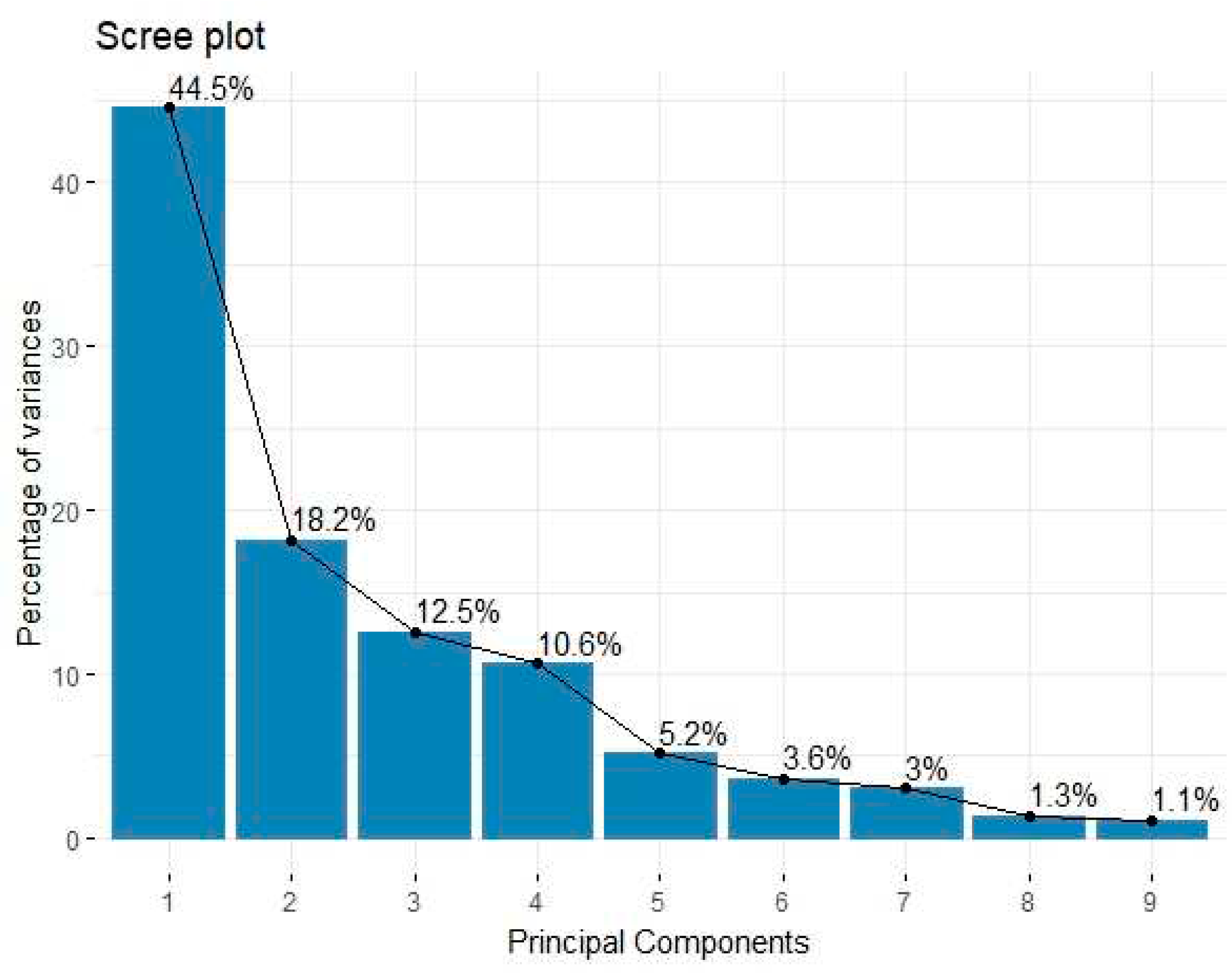
Figure 2. Protein data; PCA biplot.

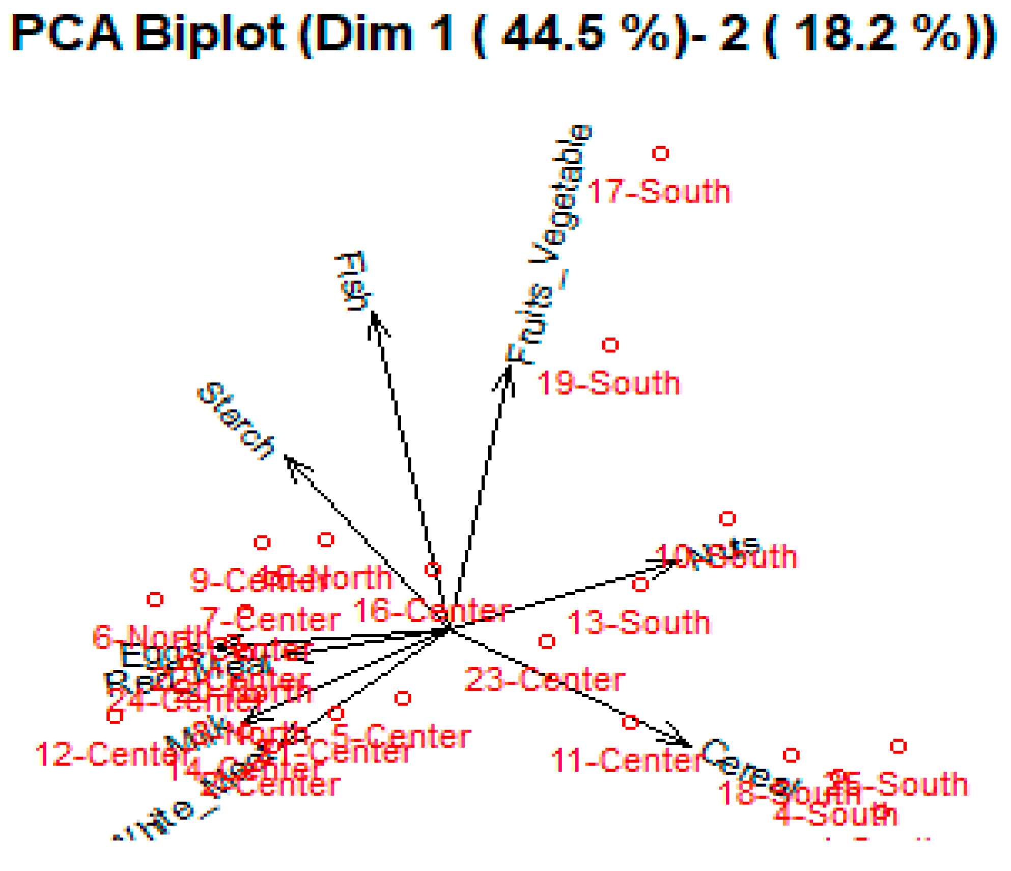
Figure 3. Protein data; variable factor map.

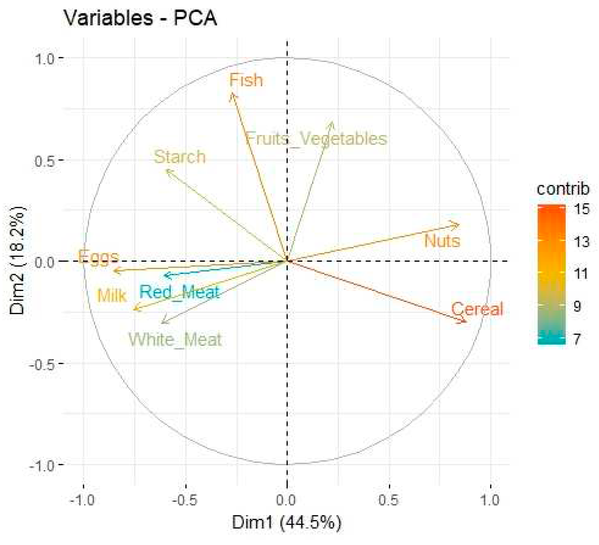
Figure 4. Protein data; PCA biplot contribution plot.

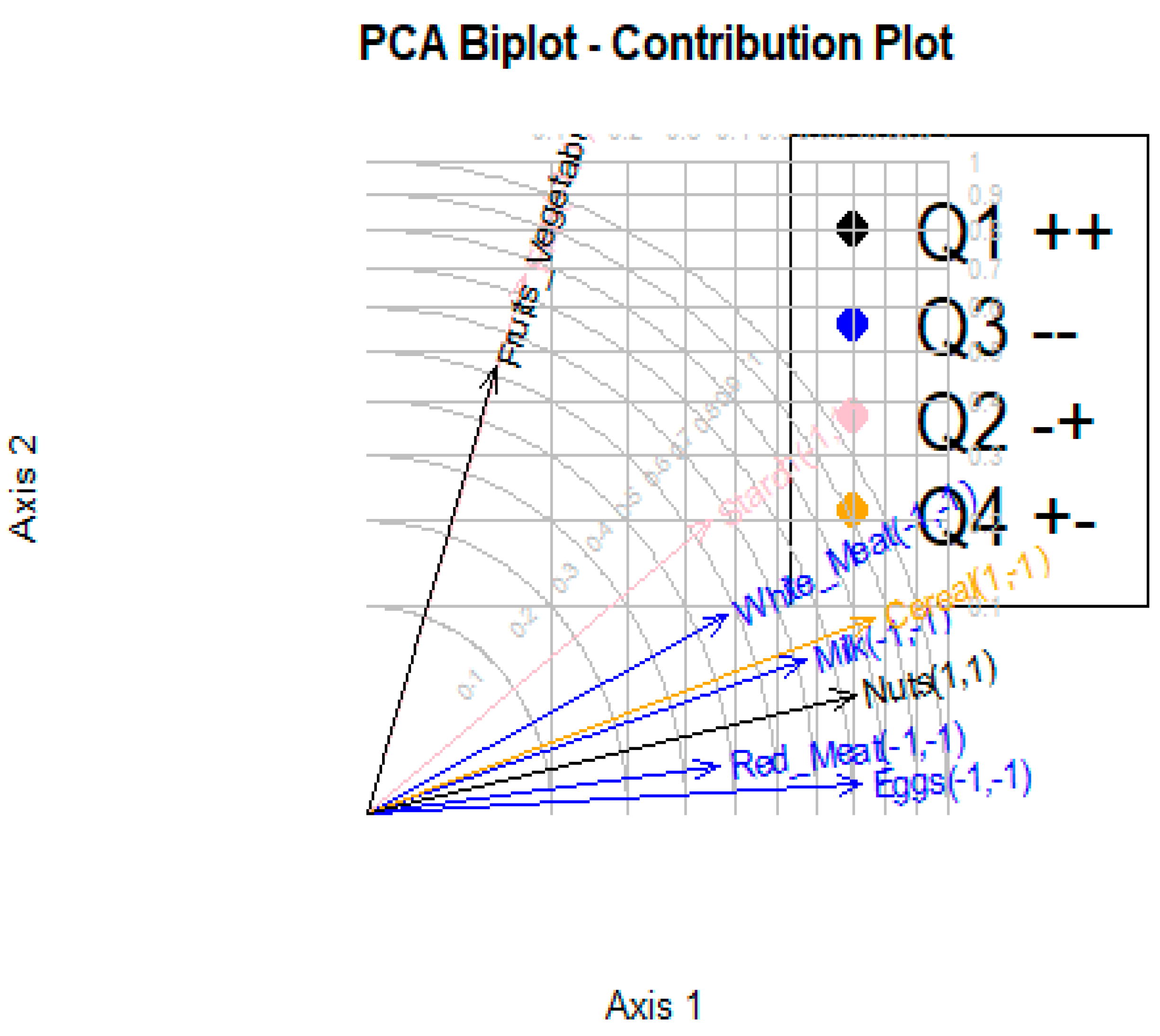
Figure 5. Chemical data; PCA scree plot.

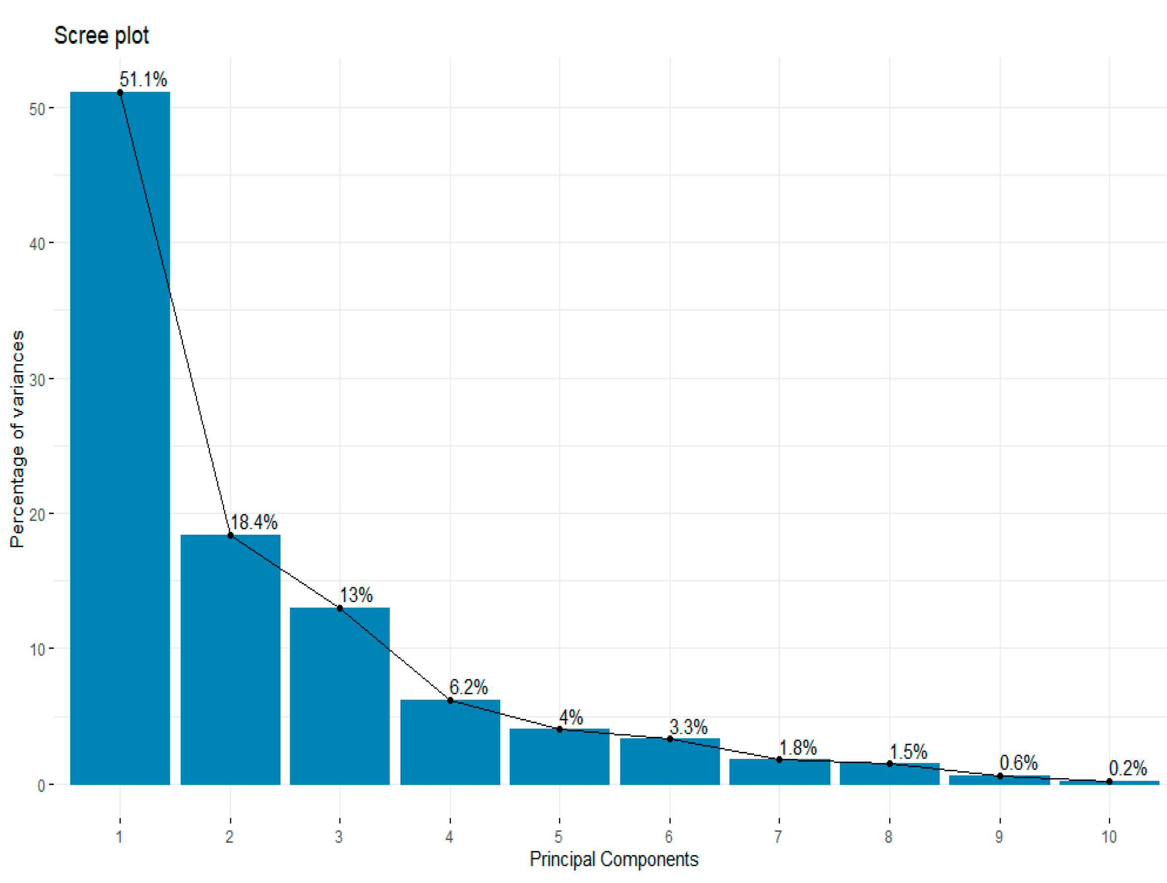
Figure 6. Chemical data; PCA biplot.

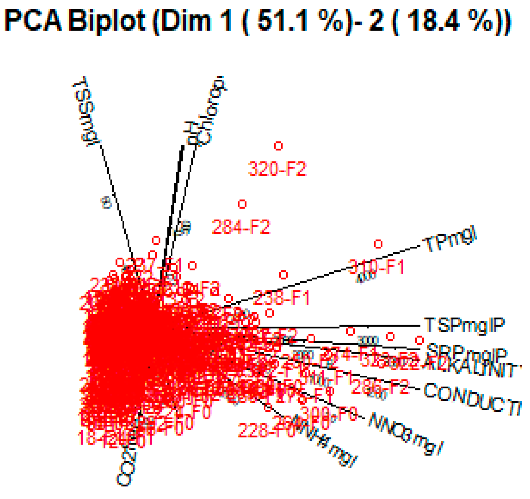
Figure 7. Chemical data; variable factor map.

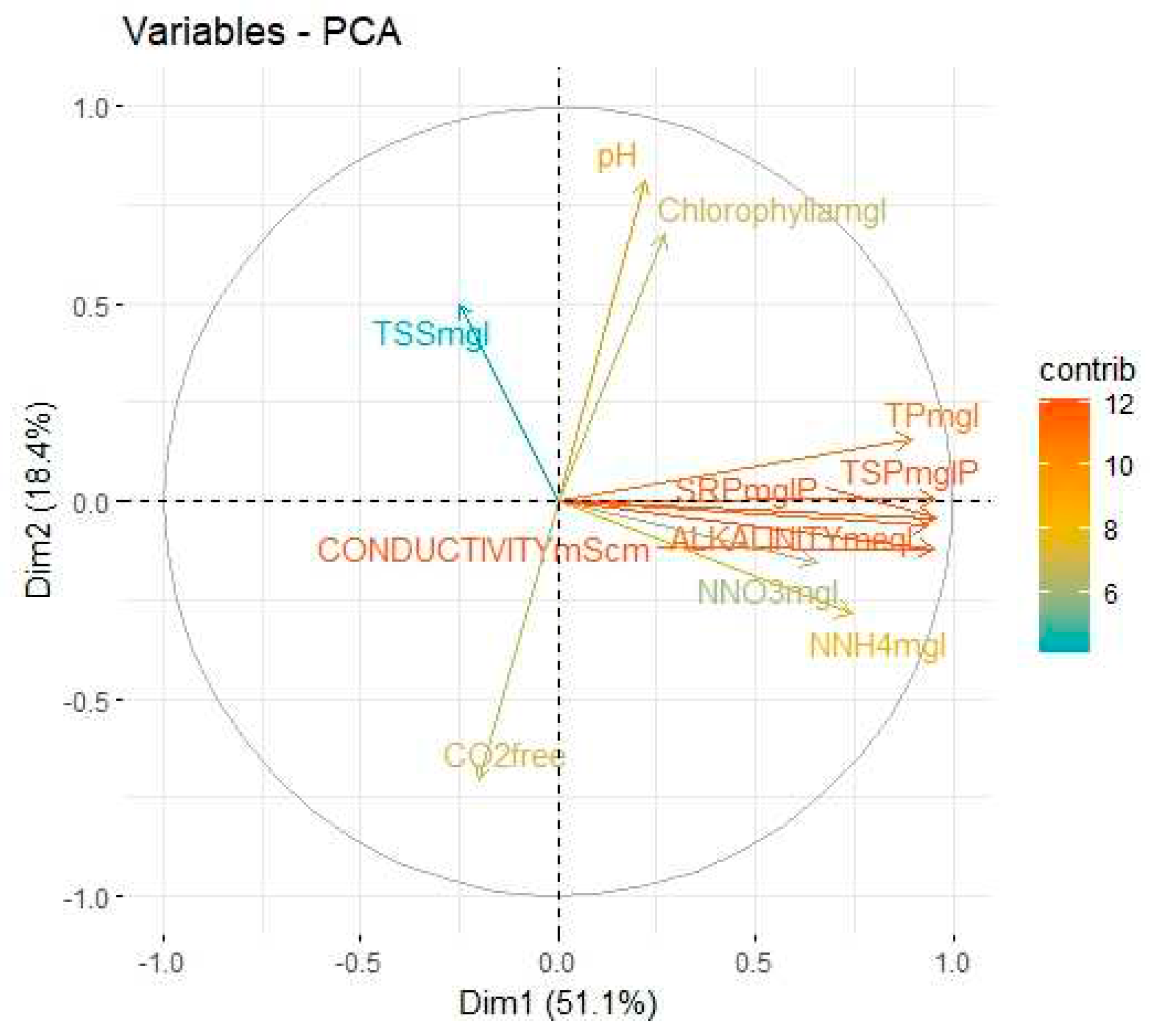
Figure 8. Chemical data; PCA biplot contribution plot.

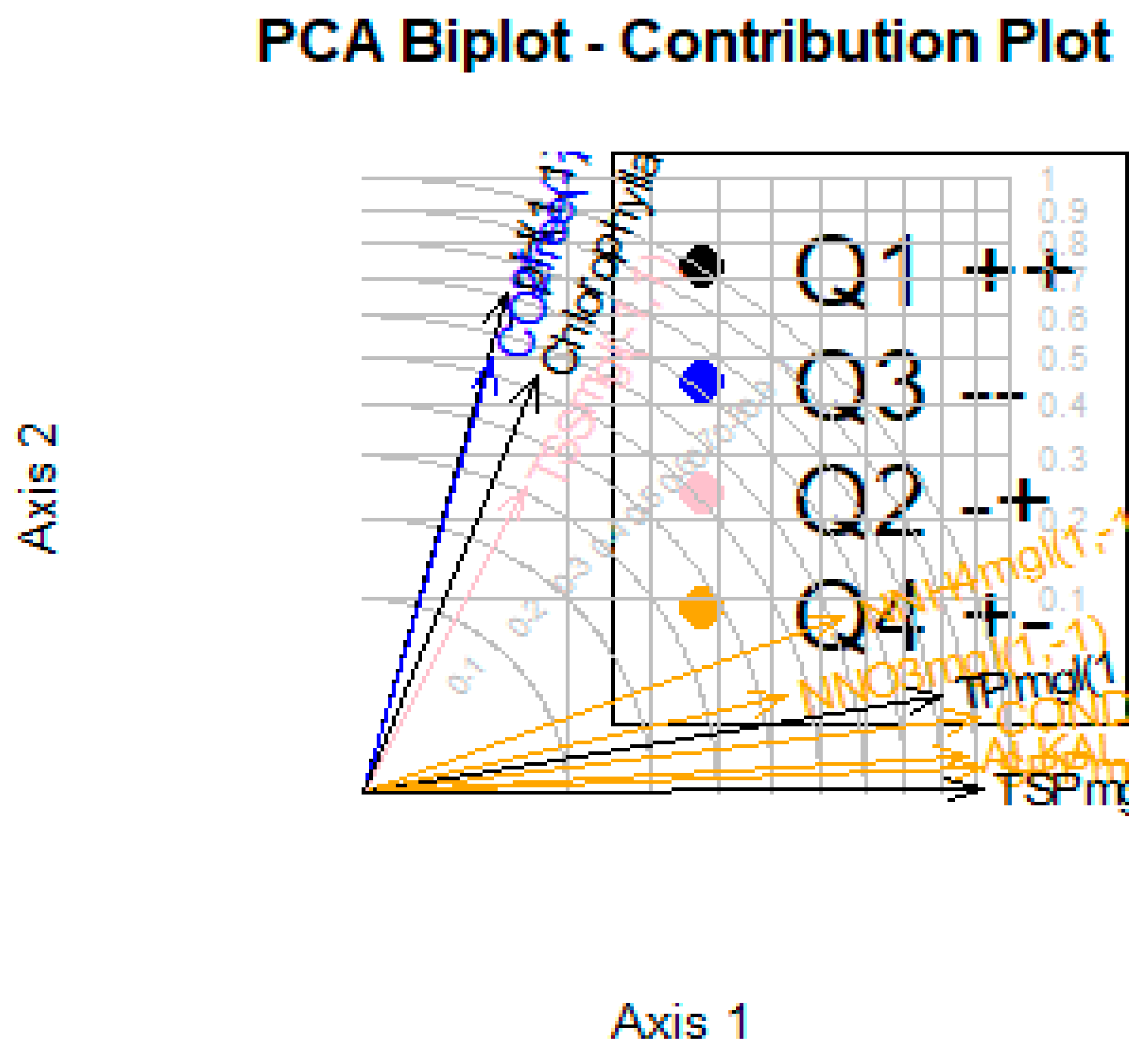
Table 1. Eigenvector coefficients of Protein data.

Variable (food)	$P C 1$	$P C 2$	$P C 3$	$P C 4$	$P C 5$
Red_Meat	-0.303	-0.056	-0.298	-0.646	0.322
White_Meat	-0.311	-0.237	0.624	0.037	-0.300
Eggs	-0.427	-0.035	0.182	-0.313	0.079
Milk	-0.378	-0.185	-0.386	0.003	-0.200
Fish	-0.136	0.647	-0.321	0.216	-0.290
Cereal	0.438	-0.233	0.096	0.006	0.238
Starch	-0.297	0.353	0.243	0.337	0.736
Nuts	0.420	0.143	-0.054	-0.330	0.151
Fruits_Vegetables	0.110	0.536	0.407	-0.462	-0.234

Table 2. Protein data; Accounted Variance.

	Initial	Bootstrap Mean	CI- P2.5	CI- P97.5	CI- MEI	CI- MES
Dim 1	-44.516	46.954	38.577	56.741	38.041	55.867
Dim 2	-18.167	19.771	14.508	26.407	13.628	25.913
Dim 3	12.532	13.015	9.343	16.828	9.219	16.811
Dim 4	10.607	8.861	5.597	12.260	5.457	12.265
Dim 5	5.154	5.028	3.119	7.589	2.750	7.306
Dim 6	3.613	3.120	1.886	4.725	1.684	4.555
Dim 7	3.018	1.872	0.946	3.039	0.778	2.967
Dim 8	1.292	0.938	0.370	1.524	0.349	1.527
Dim 9	1.101	0.441	0.080	0.953	-0.001	0.884

Table 3. Eigenvector coefficients of Chemical data.

Variable	$P C 1$	$P C 2$	$P C 3$	$P C 4$	$P C 5$
pH	0.094	0.573	0.365	0.082	0.024
ALKALINITYmeql	0.395	-0.044	-0.077	-0.199	0.127
CO2free	-0.085	-0.496	-0.486	0.216	0.013
NNH4mgl	0.314	-0.202	-0.012	-0.475	0.504
NNO3mgl	0.276	-0.110	0.258	0.726	0.414
SRPmglP	0.403	-0.029	-0.052	0.062	-0.363
TPmgl	0.378	0.112	-0.205	0.050	-0.364
TSSmgl	-0.106	0.351	-0.566	0.334	0.160
CONDUCTIVITYmScm	0.402	-0.086	0.016	0.069	0.222
TSPmglP	0.403	0.005	-0.077	0.053	-0.362
Chlorophyllamgl	0.114	0.476	-0.432	-0.167	0.295

Table 4. Chemical data; Accounted Variance.

	Initial	Bootstrap Mean	CI- P2.5	CI- P97.5	CI- MEI	CI- MES
Dim 1	51.067	51.319	49.330	53.395	49.308	53.330
Dim 2	18.355	18.465	17.150	20.068	16.997	19.932
Dim 3	12.961	12.879	11.529	14.170	11.540	14.217
Dim 4	6.191	6.284	5.262	7.424	5.170	7.399
Dim 5	4.014	4.031	3.289	4.844	3.240	4.822
Dim 6	3.296	3.118	2.516	3.700	2.519	3.716
Dim 7	1.767	1.766	1.465	2.185	1.419	2.112
Dim 8	1.476	1.382	1.033	1.693	1.049	1.715
Dim 9	0.640	0.539	0.248	0.793	0.225	0.853
Dim 10	0.197	0.184	0.108	0.295	0.092	0.277
Dim 11	0.036	0.034	0.019	0.054	0.017	0.051

Disclaimer/Publisher’s Note: The statements, opinions and data contained in all publications are solely those of the individual author(s) and contributor(s) and not of MDPI and/or the editor(s). MDPI and/or the editor(s) disclaim responsibility for any injury to people or property resulting from any ideas, methods, instructions or products referred to in the content.

© 2023 by the authors. Licensee MDPI, Basel, Switzerland. This article is an open access article distributed under the terms and conditions of the Creative Commons Attribution (CC BY) license (https://creativecommons.org/licenses/by/4.0/).

Copyright: This open access article is published under a Creative Commons CC BY 4.0 license, which permit the free download, distribution, and reuse, provided that the author and preprint are cited in any reuse.

Submitted:

15 July 2023

Posted:

17 July 2023

You are already at the latest version

Alerts

Abstract

Keywords:

Subject: Computer Science and Mathematics - Probability and Statistics

1. Introduction