
You are currently viewing a beta version of our website. If you spot anything unusual, kindly let us know.
Preprint
Brief Report
A Step Toward the Future: Using Machine Learning to Detect Leukemia.
Altmetrics
Downloads
132
Views
27
Comments
0

This version is not peer-reviewed
Application of Machine Learning in Molecular Imaging
Abstract
Leukemia is a cancer of the bone marrow, a spongy tissue that secretes into the bones and serves as the site for the production of blood cells. One of the most prevalent kinds of leukemia in adults is acute myeloid leukemia (AML). Leukemia has non-specific signs and symptoms that are also similar to those of other interpersonal illnesses. The only way to accurately diagnose leukemia is by manually examining a stained blood smear or bone marrow aspirate under the microscope. However, this approach takes more time and is less precise. This paper describes a method for the automatic recognition and classification of AML in blood smears. Classification techniques include decision trees, logistic regression, support vector machines, and naive bayes.
Keywords:
Subject: Computer Science and Mathematics - Other
1. Introduction
The identification of malignant neoplastic illness may involve microscopic examination of peripheral blood smears. Nevertheless, this type of detailed microscopic evaluation takes a lot of time, is fundamentally subjective, and is controlled by the clinical knowledge and expertise of the hematopathologist. An affordable laptop power-assisted technology for measuring peripheral blood samples must be created in order to get over these problems.
In this study, methods for machine-controlled detection and subclassification of acute lymphocytic leukemia (ALL) using image processing and machine learning techniques are proposed. The machine-controlled unwellness recognition approach heavily relies on the choice of the appropriate segmentation theme. Hence, fresh techniques are envisaged to divide the traditional images of mature white cells and malignant lymph cells into their component morphological regions.
The segmentation problem is self-addressed within the supervised framework in order to make the planned schemes viable from a practical and real-time stand point. The segmentation problem is developed as picture element classification, picture element bunch, and picture element labeling problems separately in these projected strategies, which include Gaussian Naive Bayes, Logistic Regression, Decision Tree Classifier, Random Forest Classifier, and SVM field modeling.
The effectiveness of machine-controlled classifier systems is evaluated against manual results supplied by a panel of hematopathologists using a thorough validation procedure. It is observed that conventional and malignant lymphocytes have different physical characteristics.
An affordable technology is proposed to mechanically recognize lymphoblasts and observe dead peripheral blood samples. Metameric nucleus and protoplasm sections of the white cell images were used to derive morphological, textural, and color options. In comparison to other individual models, an ensemble of Random Forest classifiers demonstrates the highest classification accuracy of 96.5%. These techniques include inexpensive categorization, nucleus and protoplasm feature extraction, and lymph cell picture segmentation.
An enhanced theme is also planned, and the results are related to use of the flow cytometer, to subtype malignant neoplastic disease blast images supported cell lineages. By using this theme, it will be possible to establish whether blast cells are myeloid or derived from body fluid. The extracted alternatives from the leukemic blast images are mapped onto one of the two teams using an ensemble of call trees. To evaluate each model’s performance, numerous studies and tests are carried out. Performance metrics, such as the precision and efficacy of the anticipated machine-controlled systems based on routine diagnostic procedures.
1.1. Leukemia
Leukemia is a collection of diverse blood-related malignancies with varying etiologies, pathophysiology, prognoses, and therapeutic responses (Bain, 2010). In today’s world, leukemia is seen as a significant problem because it can afflict anyone, including children, adults, and occasionally newborns as young as 12 months. Leukemia is one of the top 15 most prevalent types of cancer in adults, according to a World Health Organization report, while it is the most common disease in children (Kampen,2012). The next sections will explain the blood cell lineage, different forms of leukemia, diagnostic techniques now in use, available treatments, and prognostic factors in an effort to better understand leukemia.
1.2. Leukemia Types
Your doctor can identify the type of leukemia you have with the use of lab tests. The course of treatment varies for each kind of leukemia. Chronic and Acute Leukemias The name "leukemia" refers to how swiftly the disease progresses and worsens:
Acute: Typically, acute leukemia progresses quickly. Malignant neoplastic illness cells are growing rapidly, and these abnormal cells don’t function like regular white blood cells do. A bone marrow examination could reveal low quantities of healthy blood cells and a high concentration of malignant neoplastic disease cells. Blood cancer patients may have extreme fatigue, bruising easily, and frequent infections.
Chronic: The progression of chronic leukemia can be gradual. Malignant neoplastic illness cells function almost identically to regular white blood cells. The first indication of illness may not be a physical illness; instead, it may be abnormal results from a routine biopsy. The biopsy, for instance, can reveal a high concentration of malignant neoplastic illness cells. Malignant neoplastic disease cells may eventually replace healthy blood cells if they are not treated.
1.3. Myeloid and Lymphoid Leukemia’s
The afflicted kind of white blood cell is sometimes used to name leukemias:
Myeloid: Myeloid, myelogenous, or leukaemia are all terms used to describe leukemia that originates in myeloid cells.
Lymphoid: Lymphoid, lymphoblastic, or lymphocytic leukemia is a type of leukemia that develops in lymphoid cells. The lymph nodes, which swell, may become a collection point for lymphoid leukemia cells.
The Four Most Common Leukemia Types
Myeloid cells are affected by acute myeloid leukemia (AML), which spreads swiftly. Blast cells from leukemia gather in the bone marrow and blood. In 2013, an estimated 15,000 People will receive an AML diagnosis. The majority (about 8,000) will be 65 years of age or older, and about 870 children and teenagers can contract this sickness.
Rapid growth is a feature of acute lymphoblastic leukemia (ALL), which affects bodily fluid cells. Blast cells from leukemia typically gather in the blood and bone marrow. More than a dozen People have been given the diagnosis of beat 2013. The majority (almost 3,600) are children and teenagers.
Myeloid cells are affected by chronic myeloid leukemia (CML), which often develops slowly at first. The variety of white blood cells has increased, according to blood testing. Moreover, the bone marrow contains a very small variety of leukemic blast cells. CML will be identified in about 6,000 Americans in 2013. Just approximately 107 children and teenagers can have this illness, and almost 0.5 (about 2,900) will be 65 years of age or older.
Lymphoid cells are affected by chronic lymphocytic leukemia (CLL), which normally develops slowly. The variety of white blood cells has increased, according to blood testing. The traditional blood corpuscle makes the aberrant cells function almost identically. In 2013, there were 16,000 CLL diagnoses in Americans. Around 10,700 are 65 years of age or older. Almost nobody is affected by this ailment. Around 6,000 additional instances of other, less prevalent types of blood cancer are expected in 2013.
2. Proposed Experimental Method
2.1. Logistic Regression
In essence, a supervised classification algorithmic rule is what logistic regression is. The target variable (or output), y, will only accept distinct values for the provided set of alternatives (or inputs), X, during a classification problem.
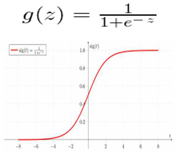
Contrary to popular assumption, a regression model could include supply regression. To determine the likelihood that a given data input belongs to the class designated as "1," the program creates a regression model. Similar to how linear regression presumes that the data follows a linear function, logistic regression uses the sigmoid function to model the data.
Only when a call threshold is taken into consideration does logistic regression transform into a classification technique. Setting the threshold value, which depends on the classification problem itself, is a crucial aspect of logistic regression.
The exactness and recall values have a negative impact on the judgment for "the price | the worth" of the threshold value. Although it would be ideal for each exactness and memory to be identical, this is rarely the case. To determine the threshold in the event of a Precision-Recall trade-off, we consider the following factors: -
- Low Precision/High Recall: We choose a call price that contains a low accuracy of exactitude or a high value of Recall in applications where we want to reduce the number of false negatives without actually reducing the amount of false positives. As an illustration, in a very cancer diagnostic application, we frequently classify any affected patient as unaffected without paying much attention to whether the patient has already received a de jure cancer diagnosis. This may be because additional medical illnesses can identify the absence of cancer, but they cannot detect the presence of the disease in a candidate who has previously been rejected.
- High Precision/Low Recall: In cases where we want to reduce the number of false positives without actually reducing the number of false negatives, we often choose a call that has a high precision value or a low recall value. For instance, if we are inclined to categorize customers based on whether or not they will react positively or negatively to a made-to-order advertisement, we would like to be absolutely certain that the consumer will react positively to the promotion because, in the event of a negative reaction, the consumer may lose out on a potential sale.
2.2. Gaussian Naive Bayes
A statistical classification method based on the Bayes Theorem is called naive Bayes. One of the only supervised learning algorithms is this one. The algorithmic rule that is quick, accurate, and dependable is the Naive Thomas Bayes classifier. For extremely large data sets, naive Thomas Bayes classifiers perform quickly and accurately. The naive Thomas Bayes classifier makes the assumption that the influence of a particular feature in a particularly class is dependent on a number of variables. A loan applicant, for instance, may or may not be interesting depending on their financial success, history of prior loans and group actions, age, and placement. These options are still considered separately even though they are interconnected. This assumption is regarded as naive because it makes calculation easier.
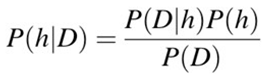
- P(h): the likelihood that hypotheses h being correct (regardless of the data). commonly known as the preceding probability of h.
- P(D): is short for probability of the data (regardless of the hypothesis). It’s commonly referred to as the prior likelihood.
- P(h|D): is the likelihood that hypothesis h is true given the facts D. Often, this is referred to as posterior probability.
- P(D|h): the likelihood of knowing d if the premise h were correct. Often, this is referred to as posterior probability.
2.3. Decision Tree Classifier
A decision tree is a tree structure that resembles a flowchart where each leaf node symbolizes the outcome and each interior node represents a feature (or attribute). In an excessive call tree, the root node at the top is recognized. It gains the ability to divide data according to attribute value. It divides the tree in a judgment call partitioning method that is extremely algorithmic. You benefit from greater cognitive process using this flowchart-like layout. It is essentially a graphic representation of a flow chart design that matches human level thinking. Decision trees are easy to understand because of this, and an interpretive response will result in the loss of a possible customer transaction.
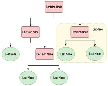
A white box form of ML algorithm is the decision tree. Internal decision-making logic is shared, but this is not the case with black box algorithms like neural networks. When compared to the neural network algorithm, it trains more quickly. The amount of records and number of attributes in the given data determine the temporal complexity of decision trees. The decision tree is a non-parametric or distribution-free strategy that does not rely on the assumptions of a probability distribution. High dimensional data can be handled by decision trees accurately.
2.4. Random Forest Classifier
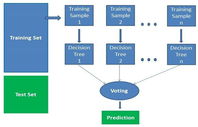
A supervised learning algorithm is random forests. Both classification and regression can be done with it. This approach is also the simplest and most adaptable. Trees comprise a forest. Using randomly chosen data samples, random forests build decision trees, extract a forecast from each tree, and then use voting to determine which answer is best. It also offers a pretty accurate indication of how important convenience is.
A supervised machine learning approach based on ensemble learning is known as random forest. A type of learning called ensemble learning involves combining the same algorithm or other algorithms to produce more accurate predictive models. The random forest algorithm creates a forest of trees by combining various algorithms of the same type, or many decision trees, hence the term "random forest". The random forest approach can be applied to both classification and regression tasks.
2.5. Support Vector Machines
Support vector classification (SVC) and support vector regression (SVR), often known as SVMs, are supervised learning algorithms that can be applied to classification and regression issues, respectively. It is only used for small datasets because processing them takes too long. We will concentrate on SVC in this set.
The fundamental assumption to make in this case is that the hyperplane is more likely to correctly classify points in its field or classes as there are more SV points from the hyperplane. Because the position of the hyperplane will change if the vector positions change, SV points are crucial in determining the hyperplane. This hyperplane is also referred to as a margin planning hyperplane technically.
Finding a hyperplane that divides characteristics into distinct domains is the foundation of SVM.
- Linear Kernel
When data can be split linearly, or along the same line, the linear kernel is employed. It is one of the most often utilized kernels. It is typically utilized when a specific data set contains a lot of properties. Text classification is one of the instances where there are too many features because each alphabet introduces a new feature. So, in Text Classification, we primarily use linear kernel.
- Radial basis function kernel (RBF)/ Gaussian Kernel:
Another well-liked kernel technique that is more frequently employed in SVM models is the Gaussian RBF (Radial Basis Function). A function whose value changes depending on how far it is from the origin or another point is the RBF kernel.
The format of the Gaussian Kernel is as follows:
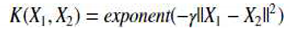
||X1 — X2 || = Euclidean distance between X1 & X2
We determine the dot product (similarity) of X1 & X2 using the distance in the initial space.
- ➢ Confusion Matrix:
A confusion matrix, also known as an error matrix, is a standard table structure that permits visualization of the performance of an algorithm, particularly one that deals with statistical classification problems.
In learning unexpectedly, a supervised learning one is typically referred to as a matching matrix. In the matrix, each row denotes a hypothetical class, whereas each column denotes occurrences in the actual class (or vice versa). The name refers to how simple it is to determine whether the system is conflating the two classes (ie usually confusing each other).
It is a particular kind of contingency table that has the same set of "classes" in both of its dimensions—"real" and "approximate"—and two dimensions (a combination of each class and dimension in the dimension table is a variable).
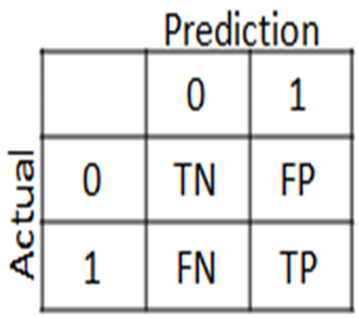
- False positive (FP) = A test result that incorrectly suggests the presence of a specific ailment or trait
- True positive (TP) = The proportion of true positivity that is successfully detected is measured by true positive (TP), which is also known as true positive rate or probability of detection in various fields.
- True Negative (TN) = The proportion of true negatives that are accurately detected is measured by True Negative (TN), also known as Specificity (also known as real negative rate).
- False Negative (FN) = False Negative (FN) results are tests that show a condition does not exist when in fact it does. An example would be a test result that shows a person does not have cancer when in fact they do.
- Steps to the work Process:
- To make writing programs easier, we import packages and libraries in the first step.
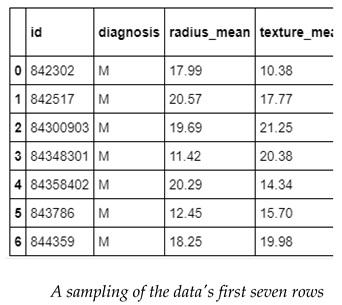
- After loading the data, I will output the first seven rows of information.
- Examine the information and determine how many rows and columns are present.
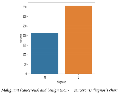
- Produce graphs and encode hierarchical data to count counts.
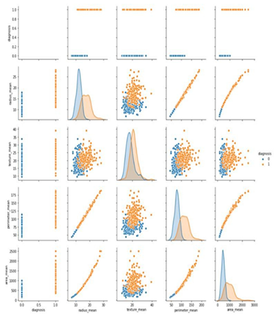
- Produce a pair plot to show the association.
- Divide the data set into a feature data set, also known as the independent data set (X), and a target data set, also known as the dependent data set, to begin setting the data for the model (Y).
- Rescale and redistribute the data.
- Provide a function that can store a variety of classification models, including logistic regression, decision trees, and random forests.
- To determine if each patient has cancer, build a model that incorporates all models and examine the accuracy scores on each model’s training data.
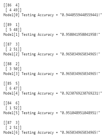
- Display the confusion matrices and model precision on test data.
- Use the model that performed best on the test data by accuracy and metric.
3. Results of Experiments and Discussion
The 569 blood samples that made up the dataset for this study were. In order to obtain the sample dataset of blood cancer for AML, which comprises of 569 and 33 different parameters on which the analysis is performed, we entered the Kaggle platform.
- Load the data
- Visualize the number
- Construct a pair plot
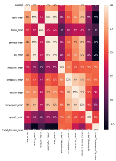
- Create a heat map to illustrate the relationship
- Display the accuracy and confusion matrices for each model on thetest data
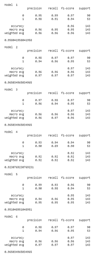
- Demonstrate more methods for obtaining classification accuracy and other metrics
- Publish the Random Forest Classifier model’s prediction along with the actual values

Table 1.
Accuracy Table.
| Method | Accuracy Percentage | ||
|---|---|---|---|
| Logistic Regression | 94.4% | ||
| K | Nearest | 95.8% | |
| Neighbour | |||
| Support Vector Machine (Linear Classifier) | 96.5% | ||
| Support | Vector | 96.5% | |
| Machine | (RBF Classifier) | ||
| Gaussian | Naive Bayes | 92.3% | |
| Decision | Tree Classifier | 95.1% | |
| Random | Forest Classifier | 96.5% | |
4. Conclusion
Create the prediction or classification based on the test data and display both the classification or prediction made by the Random Forest Classifier model and the patient’s actual values, which indicate whether or not they have cancer.
I’ve noticed that the model incorrectly diagnosed some patients as having cancer when they didn’t, and it incorrectly classified individuals who actually did have cancer as not having cancer. Even though this model is good, I want it to be even better when it comes to other people’s lives. I want it to be as accurate as possible and as good as, if not better than, doctors. So, each of the models needs to be fine-tuned a little bit further.
References
- Cristianini, N.; Shawe-Taylor, J. An Introduction to support vector machines and other kernel-based learning methods; Cambridge University Press: New York, NY, USA, 2000. [Google Scholar]
- Vapnik, V.N. The Ature of Statistical Learning Theory; Springer: New York, NY, USA, 1995. [Google Scholar]
- Madabhushi, A. Digital pathology image analysis: opportunities and challenges. Imaging Med. 2009, 1, 7–10. [Google Scholar] [CrossRef] [PubMed]
- Esgiar, A.N.; Naguib, R.N.G.; Sharif, B.S.; Bennett, M.K.; Murray, A. Fractal analysis in the detection of colonic cancer images. IEEE Transactions on Information Technology in Biomedicine 2002, 6, 54–58. [Google Scholar] [CrossRef] [PubMed]
- Yang, L.; Tuzel, O.; Meer, P.; Foran, D.J. Automatic image analysis of histopathology specimens using concave vertex graph. In Medical Image Computing and Computer-Assisted Intervention—MICCAI 2008; Springer: Berlin, Germany, 2008; pp. 833–841. [Google Scholar]
- Gonzalez, R.C. Digital Image Processing, Pearson Education India, 2009.
- Liao, S.; Law, M.W.K.; Chung, A.C.S. Dominant local binary patterns for texture classification. IEEE Transactions on Image Processing 2009, 18, 1107–1118. [Google Scholar] [CrossRef] [PubMed]
- Caicedo, J.C.; Cruz, A.; Gonzalez, F.A. Histopathology image classification using a bag of features and kernel functions. In Artificial Intelligence in Medicine, vol. 5651 of Lecture Notes in Computer Science; Springer: Berlin, Germany, 2009; pp. 126–135. [Google Scholar]
- Wu, H.S.; Barba, J.; Gil, J. Iterative thresholding for segmentation of cells from noisy images. J. Microsc. 2000, 197, 296–304. [Google Scholar] [CrossRef] [PubMed]
Disclaimer/Publisher’s Note: The statements, opinions and data contained in all publications are solely those of the individual author(s) and contributor(s) and not of MDPI and/or the editor(s). MDPI and/or the editor(s) disclaim responsibility for any injury to people or property resulting from any ideas, methods, instructions or products referred to in the content. |
© 2023 by the authors. Licensee MDPI, Basel, Switzerland. This article is an open access article distributed under the terms and conditions of the Creative Commons Attribution (CC BY) license (http://creativecommons.org/licenses/by/4.0/).
Copyright: This open access article is published under a Creative Commons CC BY 4.0 license, which permit the free download, distribution, and reuse, provided that the author and preprint are cited in any reuse.
supplementary.csv (122.27KB )
Submitted:
17 July 2023
Posted:
17 July 2023
You are already at the latest version
Alerts
supplementary.csv (122.27KB )
This version is not peer-reviewed
Application of Machine Learning in Molecular Imaging
Submitted:
17 July 2023
Posted:
17 July 2023
You are already at the latest version
Alerts
Abstract
Leukemia is a cancer of the bone marrow, a spongy tissue that secretes into the bones and serves as the site for the production of blood cells. One of the most prevalent kinds of leukemia in adults is acute myeloid leukemia (AML). Leukemia has non-specific signs and symptoms that are also similar to those of other interpersonal illnesses. The only way to accurately diagnose leukemia is by manually examining a stained blood smear or bone marrow aspirate under the microscope. However, this approach takes more time and is less precise. This paper describes a method for the automatic recognition and classification of AML in blood smears. Classification techniques include decision trees, logistic regression, support vector machines, and naive bayes.
Keywords:
Subject: Computer Science and Mathematics - Other
1. Introduction
The identification of malignant neoplastic illness may involve microscopic examination of peripheral blood smears. Nevertheless, this type of detailed microscopic evaluation takes a lot of time, is fundamentally subjective, and is controlled by the clinical knowledge and expertise of the hematopathologist. An affordable laptop power-assisted technology for measuring peripheral blood samples must be created in order to get over these problems.
In this study, methods for machine-controlled detection and subclassification of acute lymphocytic leukemia (ALL) using image processing and machine learning techniques are proposed. The machine-controlled unwellness recognition approach heavily relies on the choice of the appropriate segmentation theme. Hence, fresh techniques are envisaged to divide the traditional images of mature white cells and malignant lymph cells into their component morphological regions.
The segmentation problem is self-addressed within the supervised framework in order to make the planned schemes viable from a practical and real-time stand point. The segmentation problem is developed as picture element classification, picture element bunch, and picture element labeling problems separately in these projected strategies, which include Gaussian Naive Bayes, Logistic Regression, Decision Tree Classifier, Random Forest Classifier, and SVM field modeling.
The effectiveness of machine-controlled classifier systems is evaluated against manual results supplied by a panel of hematopathologists using a thorough validation procedure. It is observed that conventional and malignant lymphocytes have different physical characteristics.
An affordable technology is proposed to mechanically recognize lymphoblasts and observe dead peripheral blood samples. Metameric nucleus and protoplasm sections of the white cell images were used to derive morphological, textural, and color options. In comparison to other individual models, an ensemble of Random Forest classifiers demonstrates the highest classification accuracy of 96.5%. These techniques include inexpensive categorization, nucleus and protoplasm feature extraction, and lymph cell picture segmentation.
An enhanced theme is also planned, and the results are related to use of the flow cytometer, to subtype malignant neoplastic disease blast images supported cell lineages. By using this theme, it will be possible to establish whether blast cells are myeloid or derived from body fluid. The extracted alternatives from the leukemic blast images are mapped onto one of the two teams using an ensemble of call trees. To evaluate each model’s performance, numerous studies and tests are carried out. Performance metrics, such as the precision and efficacy of the anticipated machine-controlled systems based on routine diagnostic procedures.
1.1. Leukemia
Leukemia is a collection of diverse blood-related malignancies with varying etiologies, pathophysiology, prognoses, and therapeutic responses (Bain, 2010). In today’s world, leukemia is seen as a significant problem because it can afflict anyone, including children, adults, and occasionally newborns as young as 12 months. Leukemia is one of the top 15 most prevalent types of cancer in adults, according to a World Health Organization report, while it is the most common disease in children (Kampen,2012). The next sections will explain the blood cell lineage, different forms of leukemia, diagnostic techniques now in use, available treatments, and prognostic factors in an effort to better understand leukemia.
1.2. Leukemia Types
Your doctor can identify the type of leukemia you have with the use of lab tests. The course of treatment varies for each kind of leukemia. Chronic and Acute Leukemias The name "leukemia" refers to how swiftly the disease progresses and worsens:
Acute: Typically, acute leukemia progresses quickly. Malignant neoplastic illness cells are growing rapidly, and these abnormal cells don’t function like regular white blood cells do. A bone marrow examination could reveal low quantities of healthy blood cells and a high concentration of malignant neoplastic disease cells. Blood cancer patients may have extreme fatigue, bruising easily, and frequent infections.
Chronic: The progression of chronic leukemia can be gradual. Malignant neoplastic illness cells function almost identically to regular white blood cells. The first indication of illness may not be a physical illness; instead, it may be abnormal results from a routine biopsy. The biopsy, for instance, can reveal a high concentration of malignant neoplastic illness cells. Malignant neoplastic disease cells may eventually replace healthy blood cells if they are not treated.
1.3. Myeloid and Lymphoid Leukemia’s
The afflicted kind of white blood cell is sometimes used to name leukemias:
Myeloid: Myeloid, myelogenous, or leukaemia are all terms used to describe leukemia that originates in myeloid cells.
Lymphoid: Lymphoid, lymphoblastic, or lymphocytic leukemia is a type of leukemia that develops in lymphoid cells. The lymph nodes, which swell, may become a collection point for lymphoid leukemia cells.
The Four Most Common Leukemia Types
Myeloid cells are affected by acute myeloid leukemia (AML), which spreads swiftly. Blast cells from leukemia gather in the bone marrow and blood. In 2013, an estimated 15,000 People will receive an AML diagnosis. The majority (about 8,000) will be 65 years of age or older, and about 870 children and teenagers can contract this sickness.
Rapid growth is a feature of acute lymphoblastic leukemia (ALL), which affects bodily fluid cells. Blast cells from leukemia typically gather in the blood and bone marrow. More than a dozen People have been given the diagnosis of beat 2013. The majority (almost 3,600) are children and teenagers.
Myeloid cells are affected by chronic myeloid leukemia (CML), which often develops slowly at first. The variety of white blood cells has increased, according to blood testing. Moreover, the bone marrow contains a very small variety of leukemic blast cells. CML will be identified in about 6,000 Americans in 2013. Just approximately 107 children and teenagers can have this illness, and almost 0.5 (about 2,900) will be 65 years of age or older.
Lymphoid cells are affected by chronic lymphocytic leukemia (CLL), which normally develops slowly. The variety of white blood cells has increased, according to blood testing. The traditional blood corpuscle makes the aberrant cells function almost identically. In 2013, there were 16,000 CLL diagnoses in Americans. Around 10,700 are 65 years of age or older. Almost nobody is affected by this ailment. Around 6,000 additional instances of other, less prevalent types of blood cancer are expected in 2013.
2. Proposed Experimental Method
2.1. Logistic Regression
In essence, a supervised classification algorithmic rule is what logistic regression is. The target variable (or output), y, will only accept distinct values for the provided set of alternatives (or inputs), X, during a classification problem.
Contrary to popular assumption, a regression model could include supply regression. To determine the likelihood that a given data input belongs to the class designated as "1," the program creates a regression model. Similar to how linear regression presumes that the data follows a linear function, logistic regression uses the sigmoid function to model the data.
Only when a call threshold is taken into consideration does logistic regression transform into a classification technique. Setting the threshold value, which depends on the classification problem itself, is a crucial aspect of logistic regression.
The exactness and recall values have a negative impact on the judgment for "the price | the worth" of the threshold value. Although it would be ideal for each exactness and memory to be identical, this is rarely the case. To determine the threshold in the event of a Precision-Recall trade-off, we consider the following factors: -
- Low Precision/High Recall: We choose a call price that contains a low accuracy of exactitude or a high value of Recall in applications where we want to reduce the number of false negatives without actually reducing the amount of false positives. As an illustration, in a very cancer diagnostic application, we frequently classify any affected patient as unaffected without paying much attention to whether the patient has already received a de jure cancer diagnosis. This may be because additional medical illnesses can identify the absence of cancer, but they cannot detect the presence of the disease in a candidate who has previously been rejected.
- High Precision/Low Recall: In cases where we want to reduce the number of false positives without actually reducing the number of false negatives, we often choose a call that has a high precision value or a low recall value. For instance, if we are inclined to categorize customers based on whether or not they will react positively or negatively to a made-to-order advertisement, we would like to be absolutely certain that the consumer will react positively to the promotion because, in the event of a negative reaction, the consumer may lose out on a potential sale.
2.2. Gaussian Naive Bayes
A statistical classification method based on the Bayes Theorem is called naive Bayes. One of the only supervised learning algorithms is this one. The algorithmic rule that is quick, accurate, and dependable is the Naive Thomas Bayes classifier. For extremely large data sets, naive Thomas Bayes classifiers perform quickly and accurately. The naive Thomas Bayes classifier makes the assumption that the influence of a particular feature in a particularly class is dependent on a number of variables. A loan applicant, for instance, may or may not be interesting depending on their financial success, history of prior loans and group actions, age, and placement. These options are still considered separately even though they are interconnected. This assumption is regarded as naive because it makes calculation easier.
- P(h): the likelihood that hypotheses h being correct (regardless of the data). commonly known as the preceding probability of h.
- P(D): is short for probability of the data (regardless of the hypothesis). It’s commonly referred to as the prior likelihood.
- P(h|D): is the likelihood that hypothesis h is true given the facts D. Often, this is referred to as posterior probability.
- P(D|h): the likelihood of knowing d if the premise h were correct. Often, this is referred to as posterior probability.
2.3. Decision Tree Classifier
A decision tree is a tree structure that resembles a flowchart where each leaf node symbolizes the outcome and each interior node represents a feature (or attribute). In an excessive call tree, the root node at the top is recognized. It gains the ability to divide data according to attribute value. It divides the tree in a judgment call partitioning method that is extremely algorithmic. You benefit from greater cognitive process using this flowchart-like layout. It is essentially a graphic representation of a flow chart design that matches human level thinking. Decision trees are easy to understand because of this, and an interpretive response will result in the loss of a possible customer transaction.
A white box form of ML algorithm is the decision tree. Internal decision-making logic is shared, but this is not the case with black box algorithms like neural networks. When compared to the neural network algorithm, it trains more quickly. The amount of records and number of attributes in the given data determine the temporal complexity of decision trees. The decision tree is a non-parametric or distribution-free strategy that does not rely on the assumptions of a probability distribution. High dimensional data can be handled by decision trees accurately.
2.4. Random Forest Classifier
A supervised learning algorithm is random forests. Both classification and regression can be done with it. This approach is also the simplest and most adaptable. Trees comprise a forest. Using randomly chosen data samples, random forests build decision trees, extract a forecast from each tree, and then use voting to determine which answer is best. It also offers a pretty accurate indication of how important convenience is.
A supervised machine learning approach based on ensemble learning is known as random forest. A type of learning called ensemble learning involves combining the same algorithm or other algorithms to produce more accurate predictive models. The random forest algorithm creates a forest of trees by combining various algorithms of the same type, or many decision trees, hence the term "random forest". The random forest approach can be applied to both classification and regression tasks.
2.5. Support Vector Machines
Support vector classification (SVC) and support vector regression (SVR), often known as SVMs, are supervised learning algorithms that can be applied to classification and regression issues, respectively. It is only used for small datasets because processing them takes too long. We will concentrate on SVC in this set.
The fundamental assumption to make in this case is that the hyperplane is more likely to correctly classify points in its field or classes as there are more SV points from the hyperplane. Because the position of the hyperplane will change if the vector positions change, SV points are crucial in determining the hyperplane. This hyperplane is also referred to as a margin planning hyperplane technically.
Finding a hyperplane that divides characteristics into distinct domains is the foundation of SVM.
- Linear Kernel
When data can be split linearly, or along the same line, the linear kernel is employed. It is one of the most often utilized kernels. It is typically utilized when a specific data set contains a lot of properties. Text classification is one of the instances where there are too many features because each alphabet introduces a new feature. So, in Text Classification, we primarily use linear kernel.
- Radial basis function kernel (RBF)/ Gaussian Kernel:
Another well-liked kernel technique that is more frequently employed in SVM models is the Gaussian RBF (Radial Basis Function). A function whose value changes depending on how far it is from the origin or another point is the RBF kernel.
The format of the Gaussian Kernel is as follows:
||X1 — X2 || = Euclidean distance between X1 & X2
We determine the dot product (similarity) of X1 & X2 using the distance in the initial space.
- ➢ Confusion Matrix:
A confusion matrix, also known as an error matrix, is a standard table structure that permits visualization of the performance of an algorithm, particularly one that deals with statistical classification problems.
In learning unexpectedly, a supervised learning one is typically referred to as a matching matrix. In the matrix, each row denotes a hypothetical class, whereas each column denotes occurrences in the actual class (or vice versa). The name refers to how simple it is to determine whether the system is conflating the two classes (ie usually confusing each other).
It is a particular kind of contingency table that has the same set of "classes" in both of its dimensions—"real" and "approximate"—and two dimensions (a combination of each class and dimension in the dimension table is a variable).
- False positive (FP) = A test result that incorrectly suggests the presence of a specific ailment or trait
- True positive (TP) = The proportion of true positivity that is successfully detected is measured by true positive (TP), which is also known as true positive rate or probability of detection in various fields.
- True Negative (TN) = The proportion of true negatives that are accurately detected is measured by True Negative (TN), also known as Specificity (also known as real negative rate).
- False Negative (FN) = False Negative (FN) results are tests that show a condition does not exist when in fact it does. An example would be a test result that shows a person does not have cancer when in fact they do.
- Steps to the work Process:
- To make writing programs easier, we import packages and libraries in the first step.
- After loading the data, I will output the first seven rows of information.
- Examine the information and determine how many rows and columns are present.
- Produce graphs and encode hierarchical data to count counts.
- Produce a pair plot to show the association.
- Divide the data set into a feature data set, also known as the independent data set (X), and a target data set, also known as the dependent data set, to begin setting the data for the model (Y).
- Rescale and redistribute the data.
- Provide a function that can store a variety of classification models, including logistic regression, decision trees, and random forests.
- To determine if each patient has cancer, build a model that incorporates all models and examine the accuracy scores on each model’s training data.
- Display the confusion matrices and model precision on test data.
- Use the model that performed best on the test data by accuracy and metric.
3. Results of Experiments and Discussion
The 569 blood samples that made up the dataset for this study were. In order to obtain the sample dataset of blood cancer for AML, which comprises of 569 and 33 different parameters on which the analysis is performed, we entered the Kaggle platform.
- Load the data
- Visualize the number
- Construct a pair plot
- Create a heat map to illustrate the relationship
- Display the accuracy and confusion matrices for each model on thetest data
- Demonstrate more methods for obtaining classification accuracy and other metrics
- Publish the Random Forest Classifier model’s prediction along with the actual values
Table 1.
Accuracy Table.
| Method | Accuracy Percentage | ||
|---|---|---|---|
| Logistic Regression | 94.4% | ||
| K | Nearest | 95.8% | |
| Neighbour | |||
| Support Vector Machine (Linear Classifier) | 96.5% | ||
| Support | Vector | 96.5% | |
| Machine | (RBF Classifier) | ||
| Gaussian | Naive Bayes | 92.3% | |
| Decision | Tree Classifier | 95.1% | |
| Random | Forest Classifier | 96.5% | |
4. Conclusion
Create the prediction or classification based on the test data and display both the classification or prediction made by the Random Forest Classifier model and the patient’s actual values, which indicate whether or not they have cancer.
I’ve noticed that the model incorrectly diagnosed some patients as having cancer when they didn’t, and it incorrectly classified individuals who actually did have cancer as not having cancer. Even though this model is good, I want it to be even better when it comes to other people’s lives. I want it to be as accurate as possible and as good as, if not better than, doctors. So, each of the models needs to be fine-tuned a little bit further.
References
- Cristianini, N.; Shawe-Taylor, J. An Introduction to support vector machines and other kernel-based learning methods; Cambridge University Press: New York, NY, USA, 2000. [Google Scholar]
- Vapnik, V.N. The Ature of Statistical Learning Theory; Springer: New York, NY, USA, 1995. [Google Scholar]
- Madabhushi, A. Digital pathology image analysis: opportunities and challenges. Imaging Med. 2009, 1, 7–10. [Google Scholar] [CrossRef] [PubMed]
- Esgiar, A.N.; Naguib, R.N.G.; Sharif, B.S.; Bennett, M.K.; Murray, A. Fractal analysis in the detection of colonic cancer images. IEEE Transactions on Information Technology in Biomedicine 2002, 6, 54–58. [Google Scholar] [CrossRef] [PubMed]
- Yang, L.; Tuzel, O.; Meer, P.; Foran, D.J. Automatic image analysis of histopathology specimens using concave vertex graph. In Medical Image Computing and Computer-Assisted Intervention—MICCAI 2008; Springer: Berlin, Germany, 2008; pp. 833–841. [Google Scholar]
- Gonzalez, R.C. Digital Image Processing, Pearson Education India, 2009.
- Liao, S.; Law, M.W.K.; Chung, A.C.S. Dominant local binary patterns for texture classification. IEEE Transactions on Image Processing 2009, 18, 1107–1118. [Google Scholar] [CrossRef] [PubMed]
- Caicedo, J.C.; Cruz, A.; Gonzalez, F.A. Histopathology image classification using a bag of features and kernel functions. In Artificial Intelligence in Medicine, vol. 5651 of Lecture Notes in Computer Science; Springer: Berlin, Germany, 2009; pp. 126–135. [Google Scholar]
- Wu, H.S.; Barba, J.; Gil, J. Iterative thresholding for segmentation of cells from noisy images. J. Microsc. 2000, 197, 296–304. [Google Scholar] [CrossRef] [PubMed]
Disclaimer/Publisher’s Note: The statements, opinions and data contained in all publications are solely those of the individual author(s) and contributor(s) and not of MDPI and/or the editor(s). MDPI and/or the editor(s) disclaim responsibility for any injury to people or property resulting from any ideas, methods, instructions or products referred to in the content. |
© 2023 by the authors. Licensee MDPI, Basel, Switzerland. This article is an open access article distributed under the terms and conditions of the Creative Commons Attribution (CC BY) license (http://creativecommons.org/licenses/by/4.0/).
Copyright: This open access article is published under a Creative Commons CC BY 4.0 license, which permit the free download, distribution, and reuse, provided that the author and preprint are cited in any reuse.
Intelligent Neural Network Schemes for Multi-Class Classification
Ying-Jie You
et al.
Applied Sciences,
2019
High-Dimensional Analysis of Single-Cell Flow Cytometry Data Predicts Relapse in Childhood Acute Lymphoblastic Leukaemia
Salvador Chulián
et al.
Cancers,
2020
A Linear Discriminant Analysis and Classification Model for Breast Cancer Diagnosis
Marion Adebiyi
et al.
Applied Sciences,
2022


MDPI Initiatives
Important Links
© 2024 MDPI (Basel, Switzerland) unless otherwise stated